1. Introduction
Successors of the Constant Conditional Correlation (CCC-)GARCH model by
Bollerslev (
1990) have become quite popular in financial applications. For overviews of multivariate GARCH models, see
Bauwens et al. (
2006) and
Silvennoinen and Teräsvirta (
2009). The most popular time-varying conditional correlation GARCH model is the DCC-GARCH model by
Engle (
2002).
Tse and Tsui (
2002) independently developed a rather similar model called the Varying Correlation (VC-)GARCH model. Both nest the CCC-GARCH model. However, there do not exist tests for testing the CCC model against either one of them. The reason may be that when the data-generating process is the CCC-GARCH model, neither the DCC- nor the VC-GARCH model is identified. This causes problems in deriving an appropriate test.
Among multivariate regime-switching GARCH models, both the Markov-switching multivariate GARCH model (
Pelletier 2006), and the Smooth Transition Conditional Correlation (STCC-)GARCH model (
Berben and Jansen 2005;
Silvennoinen and Teräsvirta 2005,
2015) nest the CCC-GARCH model. Neither of them is identified when data are generated from the smaller model. The latter authors circumvented the identification problem and developed a Lagrange multiplier type test of CCC-GARCH against STCC-GARCH.
In the meantime, GARCH equations of the CCC-GARCH model have been extended to accommodate potential nonstationarity in the series to be modelled. This has, to a large extent, been done through the so-called multiplicative decomposition of the variance of an individual series into the customary conditional variance and a deterministic component. Contributions include
Feng (
2004,
2018);
van Bellegem and von Sachs (
2004);
Engle and Rangel (
2008);
Amado and Teräsvirta (
2008,
2013,
2017);
Brownlees and Gallo (
2010) and
Mazur and Pipień (
2012).
Amado and Teräsvirta (
2014) incorporated this feature into CCC-, DCC- and VC-GARCH models. For a recent review, see
Amado et al. (
2019). The problem for which multiplicative decomposition offers a solution is that many sufficiently long return series are nonstationary in the sense that the amplitude of volatility clusters that GARCH is designed to parameterise is not constant over time. The purpose of the deterministic component in the decomposition is to rescale the observations such that the rescaled series can be described by a standard weakly stationary GARCH model.
Silvennoinen and Teräsvirta (
2021) retained the multiplicative decomposition of variances and, in addition, assumed that the correlations of their smooth transition correlation model were changing deterministically over time. As opposed to the DCC- and VC-GARCH, this allows systematic changes in correlations. For example, correlations may change from one level to another and remain there.
Hall et al. (
2021) derived a test of CCC-GARCH against this Time-Varying Correlation (TVC-)GARCH model. A drawback of their test, called the HST-test for short, is that if the dimension of the model is large, the null hypothesis of the test will also be quite large. This limits the applicability of the HST-test in practical, large dimensional applications. In this paper we develop a parsimonious alternative to the HST-test. The main thrust is to use the spectral decomposition of the correlation matrix, thereby making the eigenvalues rather than individual correlation parameters the focal point of the test. As with the HST-test, while the statistic here has been derived using a linear time trend as a transition variable, it can be generalised to detect variation in correlations according to other variables of interest, see
Silvennoinen and Teräsvirta (
2015). As a consequence, both of these tests are designed to detect correlation movement as a function of the chosen transition variable, making them flexible in practical applications. The test presented in this paper does have a difference compared to the HST test: the alternative hypothesis is generally not a correlation matrix. The resulting test may therefore be viewed as a general misspecification test of the CCC-GARCH model when the correlations are allowed to change systematically over time.
The plan of the paper is as follows.
Section 2 contains an overview of previous tests of constant GARCH equations and correlations. The model and the null hypothesis to be tested are also presented there. The log-likelihood, score and the information matrix can be found in
Section 3 and
Section 4 and the test statistic in
Section 5. In
Section 6, the performance of the test in finite samples is examined by simulation, including a few cases in which the GARCH equations are misspecified.
Section 7 contains a real-world application. Conclusions can be found in
Section 8. Proofs and further simulation evidence are relegated to an appendix.
2. Previous Literature and the Time-Varying Smooth Transition Correlation GARCH Model
Before considering our Time-Varying Smooth Transition Correlation (TV-STC-GARCH) model, we take a quick look at the literature on tests of constancy of the error covariance matrix of a possibly nonlinear vector model. This literature is not very large, and rather few tests actually focus on the correlation matrix. There exist tests against conditional heteroskedasticity.
Lütkepohl (
2004, pp. 130–131) constructed a test of no multivariate ARCH against multivariate ARCH of order
q. This Lagrange multiplier test works best when
q and
N, the dimension of the model, are small. The test statistic has an asymptotic
-distribution with
degrees of freedom when the null hypothesis of no ARCH holds.
Eklund and Teräsvirta (
2007) designed a test in which the covariance matrix
is decomposed as in
Bollerslev (
1990) such that
where
is a time-varying matrix with positive diagonal elements and
is a positive definite correlation matrix. The null hypothesis is that
where
,
. The alternative is
at least for one
i. Typically
, where both the (parametric) function
and the argument
can be defined in various ways. The restriction that
is constant saves degrees of freedom but in some situations has a negative effect on the power of the test.
A similar decomposition is employed by
Catani et al. (
2017), but the purpose of their test is more limited. The decomposition has the form
, where
such that
,
, are ARCH- or GARCH-type conditional variances. For example,
where
is an indicator variable, with
,
,
, and
, so (
1) has a GJR-GARCH structure, see
Glosten et al. (
1993). Furthermore
where
, and
. The null hypothesis H
:
, or
,
, which means that after estimating the CCC-GARCH model, there is no structure unmodelled in conditional variances. When
, this test may be viewed as a parsimonious version of Lütkepohl’s test of no multivariate ARCH. The authors point out that their test can also be interpreted as a generalisation of the more parsimonious test by
Ling and Li (
1997).
The aforementioned tests are tests of
such that in the decomposition
or
, it is assumed
, and the hypothesis to be tested has been
. In this work the focus is on testing H
:
. Assuming
,
Tse (
2000) derived a portmanteau type constancy test of this hypothesis and found that it has reasonable power against the alternatives he was interested in.
Péguin-Feissolle and Sanhaji (
2016) proposed two portmanteau tests that are in fact extensions to Tse’s test. The authors showed by simulation that the power of their tests is superior to that of Tse. A common feature of these tests is that the alternative is not a correlation matrix.
The TV-STC-GARCH model is a multivariate GARCH model with time-varying GARCH equations and correlations
where
is a stochastic
vector and
is an
conditional covariance matrix of
, typically the vector of returns in applications. The diagonal matrix
is a matrix of square roots of positive-valued deterministic components to be defined below and
contains the conditional standard deviations of
, where
. In what follows it is assumed that the elements of
have a first-order GJR-GARCH representation, see
Glosten et al. (
1993):
. Furthermore, in
,
with
, where
and
such that
. Note that
is assumed known to solve the identification problem arising from both
and
having an intercept. It is often convenient to set
, but any positive constant will do. Finally,
is a positive definite deterministically varying covariance matrix of
, and
. For the purposes of this paper it is assumed that
is rotation invariant:
, where the matrix
holds the time-invariant eigenvectors as its columns, and the time-varying eigenvalues are
with
If changes in the elements of
are assumed monotonic, the exponent of order one in (
6) is sufficient. If nonmonotonicity is allowed, a second-order exponent is necessary. Further note that these elements are required to be positive and sum up to
N. It is assumed that the elements of the diagonal matrix
satisfy the same conditions, and the elements of the diagonal matrix
sum up to zero. When
, it is assumed that
is a positive definite correlation matrix, in which case
is a slightly generalised version of the decomposition of the conditional covariance matrix
Bollerslev (
1990) suggested.
Hall et al. (
2021) derived a constancy test in a more general situation in which
where
is defined as in (
6) and
and
are two positive definite correlation matrices. In that set-up, as a convex combination of these two matrices
is always a positive definite correlation matrix. Their Lagrange multiplier test statistic of the null hypothesis
, i.e.,
, is asymptotically
-distributed with
degrees of freedom when the null hypothesis holds.
Even here, the focus is on testing
against the alternative that the matrix varies deterministically with time. As already indicated,
is not a correlation matrix when
. Testing constancy of
in this framework is motivated by the fact that the test of the null hypothesis H
:
in (
6) involves fewer parameters than the test of
Hall et al. (
2021) when
. It may be viewed as a parsimonious version of their test, which is an advantage when
N becomes large. When H
holds,
, and
. It is seen from (
5) and (
6) that in that situation the covariance matrix (
5) is not identified. Both
,
and
are unidentified nuisance parameters.
In order to derive a test of this null hypothesis, we circumvent the identification problem as in
Luukkonen et al. (
1988) and develop
into a Taylor series around the null hypothesis. After reparameterising, (
5) becomes
where
is a residual matrix and
,
. Requiring the diagonal elements of
to sum up to
N implies that
and
for
. Under H
,
. The elements
,
;
, in (
7) are of the form
,
,
, so the new
-dimensional null hypothesis is H
:
.
Since we shall construct a Lagrange multiplier test that only requires estimating the model under the null hypothesis we can ignore the diagonal residual matrix
because its diagonal is a null vector when H
(or H
) holds. It does contribute to the power of the test when the alternative is true. This leads to the following auxiliary covariance matrix:
Matrix (
8) is a correlation matrix only under H
, and its purpose is to function as a basis for a test of constant correlations. We call the model (
2) in which (
5) is replaced by (
8), the
auxiliary time-varying correlation GARCH model. It is a device constructed to derive the test and not a data-generating process. Its log-likelihood and score are considered in the next section.
The test we propose is similar to the one by
Yang (
2014) in that both make use of the spectral decomposition of
. It should be noted, however, that
Yang (
2014) did not decompose the covariance matrix further into conditional variances and correlations. He constructed instead a test of constancy of the covariance matrix based on this decomposition. Our work may therefore be also seen as a variant of or an extension to
Yang (
2014).
5. Test Statistic
Under regularity conditions,
Silvennoinen and Teräsvirta (
2021) showed that the maximum likelihood estimators of the parameters of the null model (time-varying GARCH equations and constant correlations) are consistent and asymptotically normal. Rewrite (
13) as
where
with
,
. Then
and
Let
and
Using the Lagrange multiplier principle and the assumption that
is multivariate normal, we obtain the following statistic for testing H
:
,
:
where
, and
where
is the estimate of
under H
. In addition, in (
16)
, where
contains square roots of the estimated deterministic components,
contains the estimated conditional standard deviations of
, and
is the
jth eigenvector of the estimated correlation matrix
under
. Based on the results in
Silvennoinen and Teräsvirta (
2021), this statistic has an asymptotic
-distribution with
degrees of freedom when H
holds. To make it operational, the blocks of the information matrix in (
15) have to be replaced by their consistent estimators.
If the transition function (
6) is assumed monotonic in
, that is,
, the second-order component can be omitted from the approximation (
7), and the
-dimensional null hypothesis becomes
. If this assumption holds, the power of the test increases compared to the situation in which the second-order component is included in the test.
As already discussed, the matrix
is a correlation matrix only when
, that is, when
. There is one exception to this rule, however. When all correlations are equal, the time-varying matrix
remains a correlation matrix when
is defined as in (
5). In the GARCH context this type of equicorrelation is discussed in
Engle and Kelly (
2012).
The test statistic (
15) can be applied in the general case in which the GARCH component is multiplicative and contains a smooth deterministically varying component. The purpose of this component,
in (
2), is to account for nonstationarity in variance that manifests itself in changing amplitudes of the volatility clusters that ARCH and GARCH models are designed to explain. A cruder way of describing this type of variability is to assume that there are breaks in the variance. This alternative does not fit into the present analysis, however, because breaks at unknown points of time make the log-likelihood ill-behaved. Nevertheless, the statistic (
15) does have power against that alternative, although the standard asymptotic theory does not cover it.
If it is assumed that
and that the GARCH process is weakly stationary, the test statistic continues to be valid. This simplifies the expressions, while the null hypothesis remains unchanged. Setting
makes it possible to test constancy of
before specifying the conditional variances. This is discussed in
Silvennoinen and Teräsvirta (
2021). If both
, the test is a parsimonious test of constancy of a correlation matrix against the alternative that the correlations change over time. In that case,
may be a covariance matrix and not necessarily a correlation matrix. The statistic (
15) must, however, be modified because the restriction that the eigenvalues sum up to
N does not hold for the covariance matrix. With this modification, the test can for instance be used for testing constancy of the error covariance matrix of a vector autoregressive model against deterministically changing covariances; see also
Yang (
2014).
6. Simulations
In this section we investigate the properties of our test via several simulations. The finer details of the various experiments as well as the tabulated results are found in
Appendix C.
We first simulate the size of our test. For this purpose, we choose
and
in (
2). All GARCH(
) equations are standard symmetric GARCH ones, parameterised such that the persistence is
and kurtosis of
,
, or in the next set up, kurtosis of
,
. For these simulations,
, and the unconditional variance is fixed to one by defining
. The correlation matrix is an equicorrelation matrix (
Engle and Kelly 2012) with either
or
, and we call the model the Constant Equicorrelation (CEC-) GARCH model. Finally,
.
The test statistic has been derived such that the highest order in the Taylor expansion equals two. In simulations, we include the orders up to four. This is done to find out how the empirical size of the test behaves when flexibility of the statistic (and the dimension of the null hypothesis) is increased to cover more variable and nonmonotonic shifts in correlations. In practice this means that (
7) becomes
where
is the residual. The null hypothesis is H
:
.
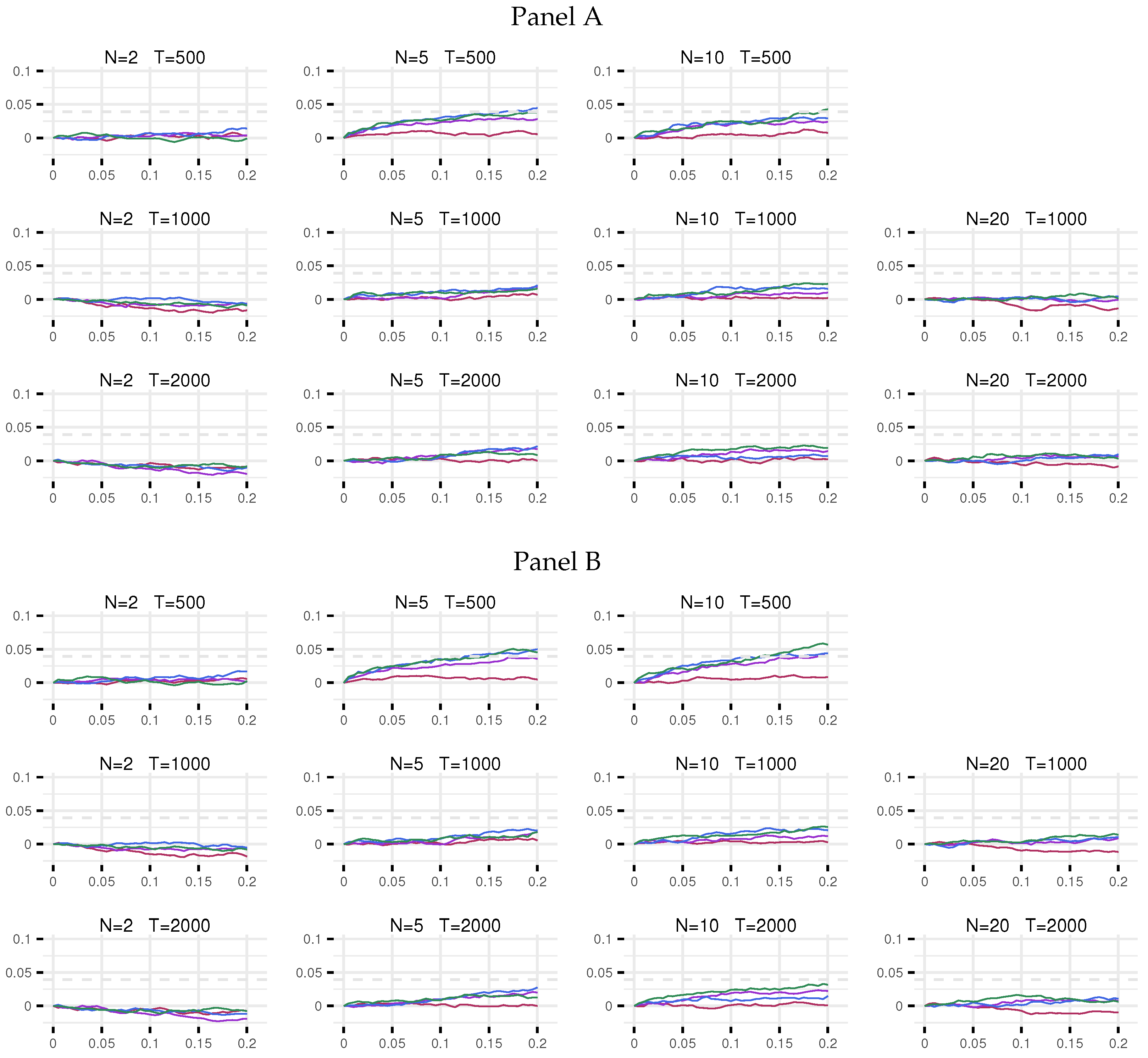
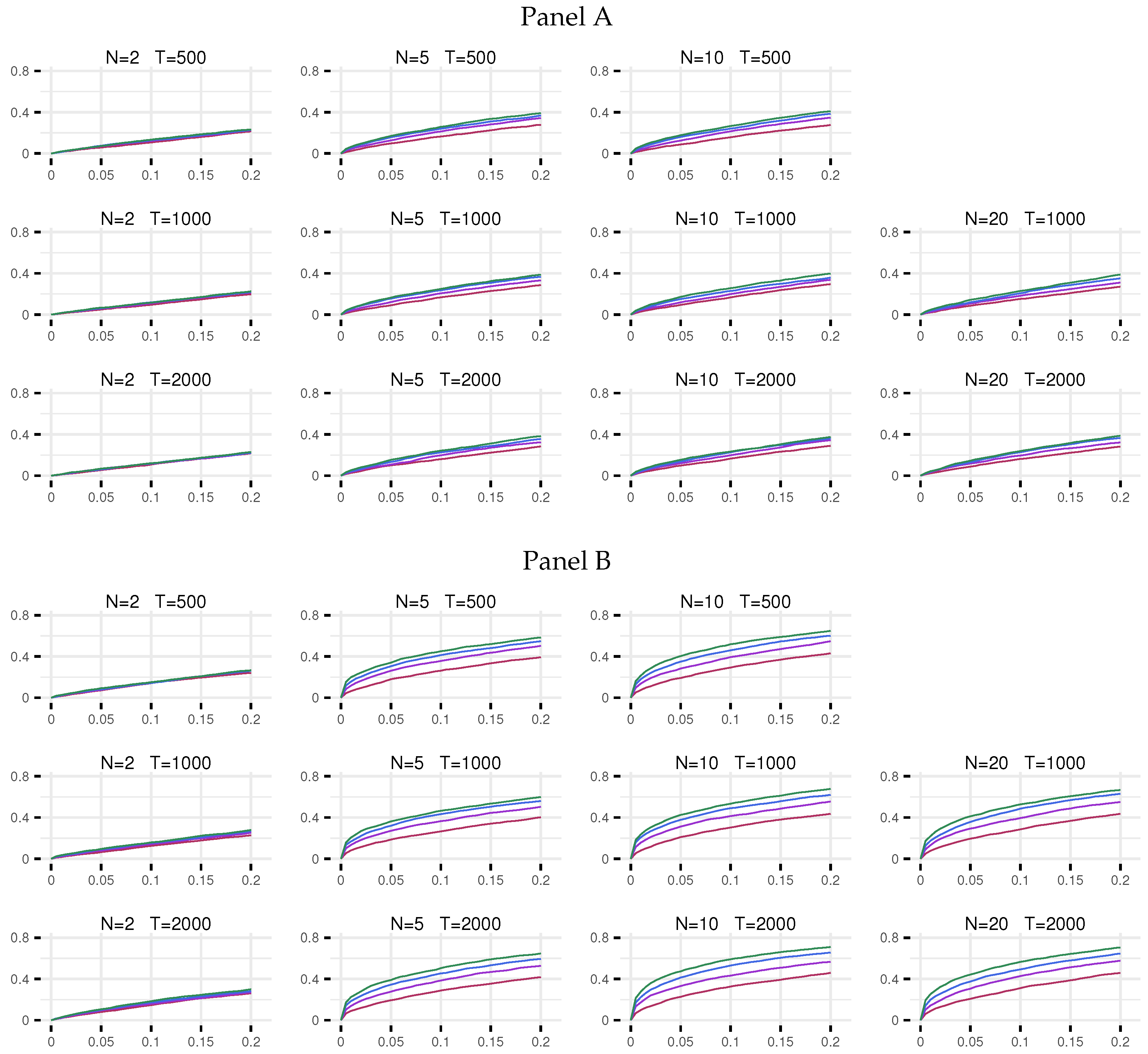
The
p-value size discrepancy, see
Davidson and MacKinnon (
1998), results for
and for kurtosis of
equal to 4 and 6, when
appear in
Figure 1 and
Table A6. Although estimating GARCH equations when
cannot be recommended in practice, this sample size is included in simulations to find out how the test behaves in that situation. The empirical size of the test is very close to its nominal size. In particular, the change in kurtosis does not have any effect on the empirical size. The only exception where the test is slightly oversized is the design in which
and the order of the polynomial is four.
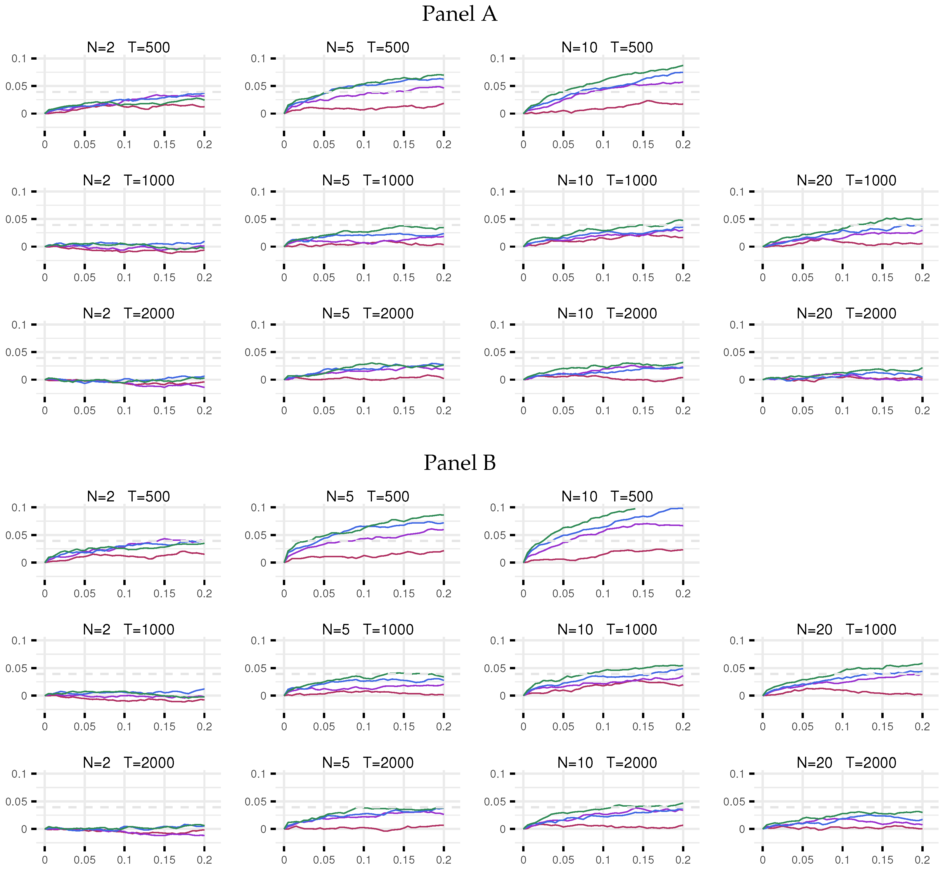
We move on to the strongly correlated situation, that is,
. The size discrepancies are in
Figure 2, see also
Table A7. The story remains, for most parts, similar to that of the weakly correlated system. Now the test is somewhat oversized when
and the Taylor polynomial is at least equal to two. The equicorrelation matrix becomes gradually more ill-conditioned as its dimension grows but is still reasonably accurately inverted when
.
Furthermore, we consider a situation where we replace the equicorrelation matrix with a positive definite matrix comprised of equicorrelation blocks. The block-equicorrelation structure (
Engle and Kelly 2012) imposes different equicorrelations between and within blocks of series. We choose
and
and blocks of size four. The chosen correlation strengths mimic those of the equicorrelated (weak and strong) levels while maintaining similar condition numbers to ensure fair comparison.
1 The only difference in
Table A8 compared to the equicorrelation case (
Table A6 and
Table A7) is that the test is slightly oversized when the order of the polynomial exceeds one.
The remaining results address misspecified GARCH equations. Such misspecification may show up in the covariance as time-variation, even if the correlations happen to be constant. The purpose of these simulations is to find out how well our test is able to detect the resulting time-variation in the eigenvalues.
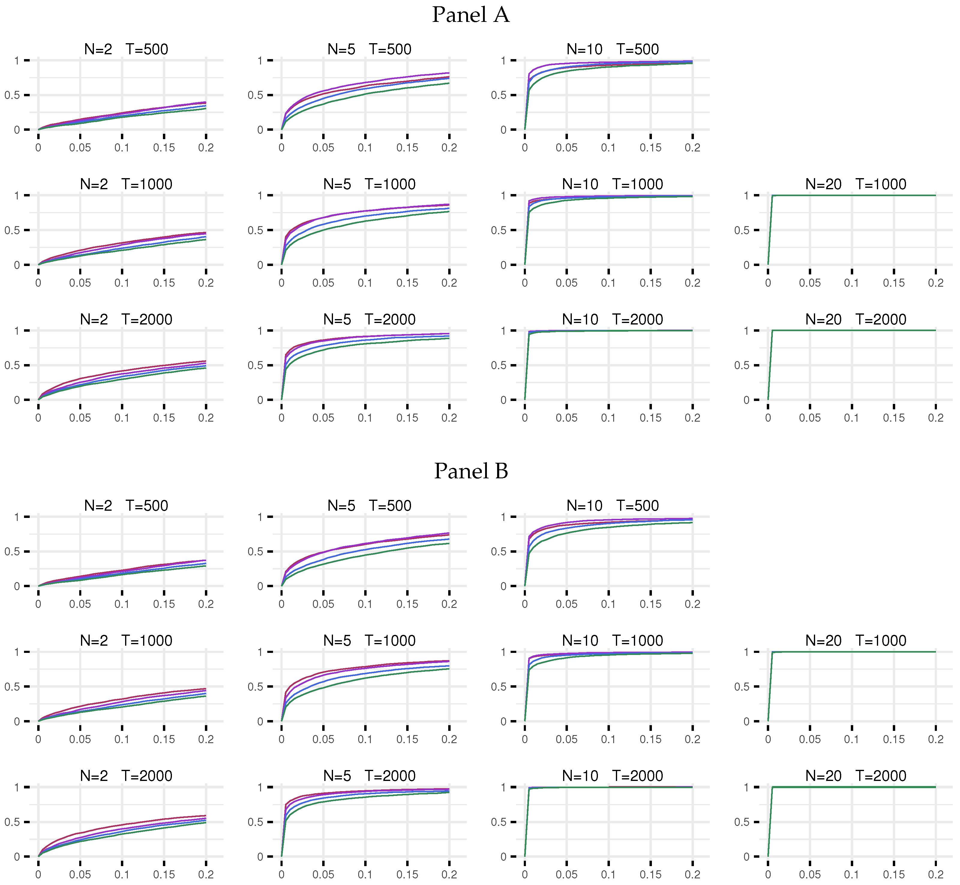
When
is time-varying but this variance is ignored, the model is indeed misspecified. In these simulations, the GARCH equations are TV-GARCH equations with
,
,
and
, with equicorrelation coefficient equal to
and
. The slope parameter
has been calibrated such that the monotonically increasing
remains practically equal to zero until
and (almost) reaches one when
. This means that there is a rather mild shift in the (local) unconditional variance in these equations over time, resulting in the amplitude of clusters doubling in size over time. The error covariance matrix is thereby time-varying, whereas the error correlation matrix is constant over time. The reported rejection frequencies in
Table A9 indicate that the test detects time-variation even for weakly correlated system (see also
Figure 3), and even more so with the correlation of
(
Table A10), which stresses the importance of specifying the GARCH equations properly before testing constancy of correlations. The rejection frequency increases with the sample size and the dimension of the system, and becomes overwhelming when more information against the null hypothesis becomes available. We also experimented with higher values of
, but because the feature is already well illustrated for
we do not report any additional results here.
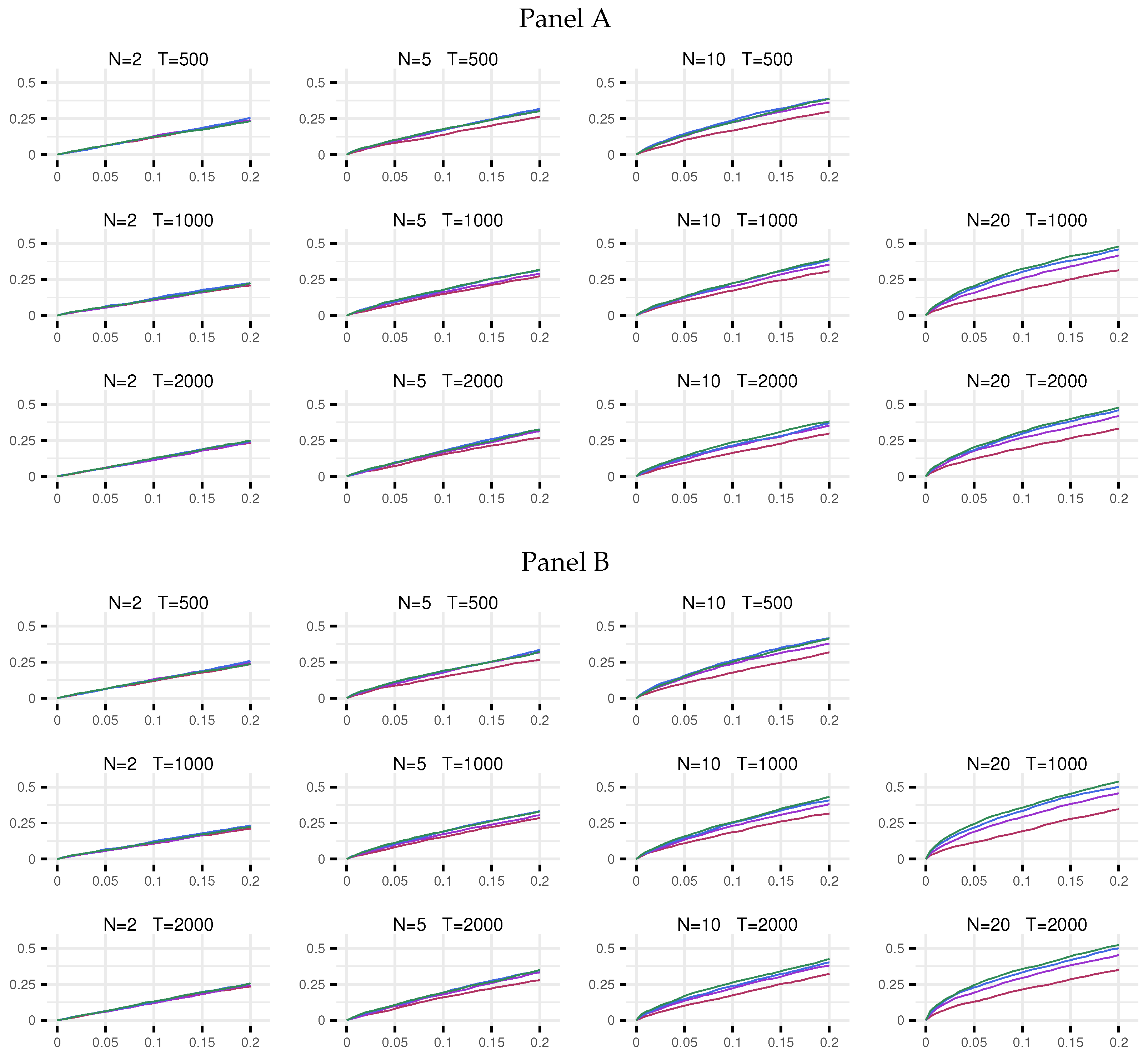
GARCH can also be misspecified such that asymmetry in the form of GJR-GARCH is ignored. The simulation design concerning this sets the
leaving the asymmetric component
solely responsible for the effect of the past shocks. The parameterisation follows the targets of the previous simulations, that is, the implied kurtosis of four and six, unconditional variance of one and persistence is kept at
. When the equicorrelation is
, there is positive size distortion for
, and for each
N, an increase in sample size makes very little difference in terms of improving the size. This is seen from the rejection frequencies reported in
Table A11, see also
Figure 4. The size distortion is already present when
for the
equicorrelated case, see
Table A12. In situations where the past shocks feed into the volatility via both symmetric and asymmetric channels, the size distortion is milder than in the extreme case discussed here, and will lie somewhere between the results here and those in
Table A6 and
Table A7. Regardless, it may be concluded that a misspecification in the GARCH equation has a minor impact on constant correlation detection in comparison to the case when the deterministic shift in GARCH is erroneously ignored.
Yet another type of misspecification occurs when there are volatility spillovers between equations that are ignored while correlations remain constant. To this end we employ an equicorrelation version of the Extended CCC-GARCH (ECCC-GARCH) model of
Jeantheau (
1998) that use CEC with
and
. Applications of the ECCC-GARCH model typically involve rather few series, and we therefore limit our simulations to systems of dimension 2, 3, and 5. The first spillover pattern is a circular one, where the past shocks travel from one volatility to another in a sequence through the system. In the second pattern the spillover shock comes from a single series and enters volatility of all the other series. For details, see
Appendix C. The results in
Table A13 and
Table A14 indicate some size distortion which is, as before, larger the stronger the correlation and also increases with the order of the polynomial used in the test. In these simulations the size distortion is of lesser magnitude than what it was in the previous experiment, where the asymmetry of the GARCH was ignored. It can, however, be expected to vary with the strength of the spillover effect.
Finally,
Table A15 and
Table A16 and
Figure 5 show what happens when, instead of normal, the error vectors are
t-distributed with
and
. Not accounting for this and assuming that the errors are multinormal, causes positive size distortion. Again, the distortion is not very large compared to what is observed in connection with ignoring the time-variation. It increases when the tails grow fatter (degrees of freedom decrease from eight to five) and when the order of the polynomial in the test grows. It may be noted, however, that this design may not be completely realistic. In practice it is quite possible that the GARCH residuals of equation
i may seem to follow a
t-distribution just because the GARCH component is misspecified, for example by ignoring the deterministic component
. Here we simulate the case in which the standard GARCH equation with normal errors for some unknown reason does not adequately describe the conditional variances. Once again, these results suggest that the GARCH equations have to be correctly specified before testing constancy of correlations can be attempted.
It is worth mentioning that when (
3) is valid, the error covariance matrix is nonconstant even when the correlations are constant. In that case, the test by
Yang (
2014) would no doubt reject the null hypothesis of a constant error
covariance matrix, whereas our test, after modelling the time-varying error variances, would not reject constancy of the error
correlation matrix.
Results of these simulations underline the need of testing adequacy of the GARCH model (constancy, asymmetry spillover effects) before embarking on testing constancy of correlations. There is another very large class of extensions to the standard GARCH model not mentioned yet, namely the GARCH-X model, see
Han and Kristensen (
2014). Within this class the possibilities of misspecification are almost limitless, and in practice the set of potential exogenous variables has to be restricted by theory considerations. We have therefore refrained from simulating designs involving ignored exogenous variables in the GARCH framework.
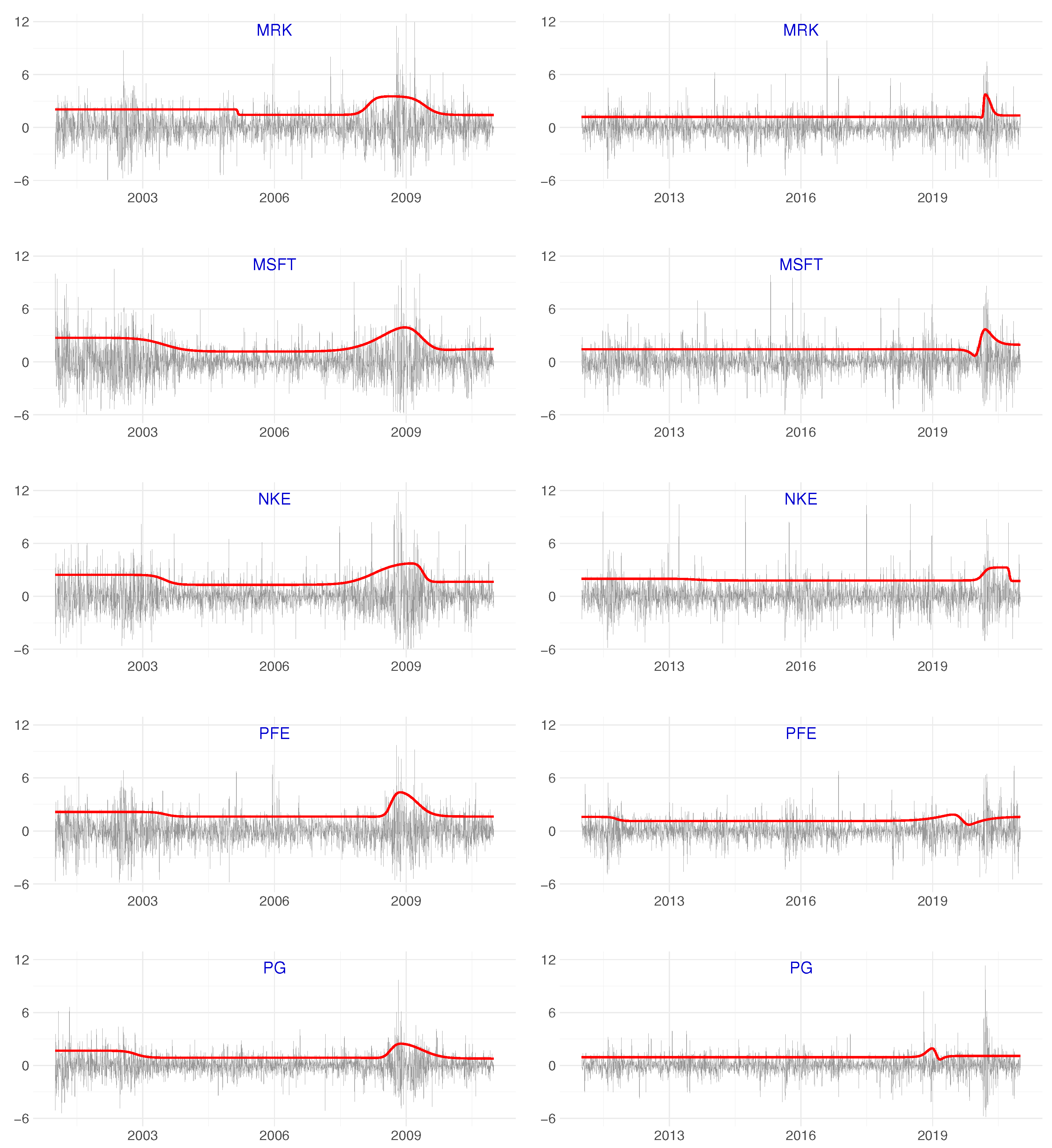
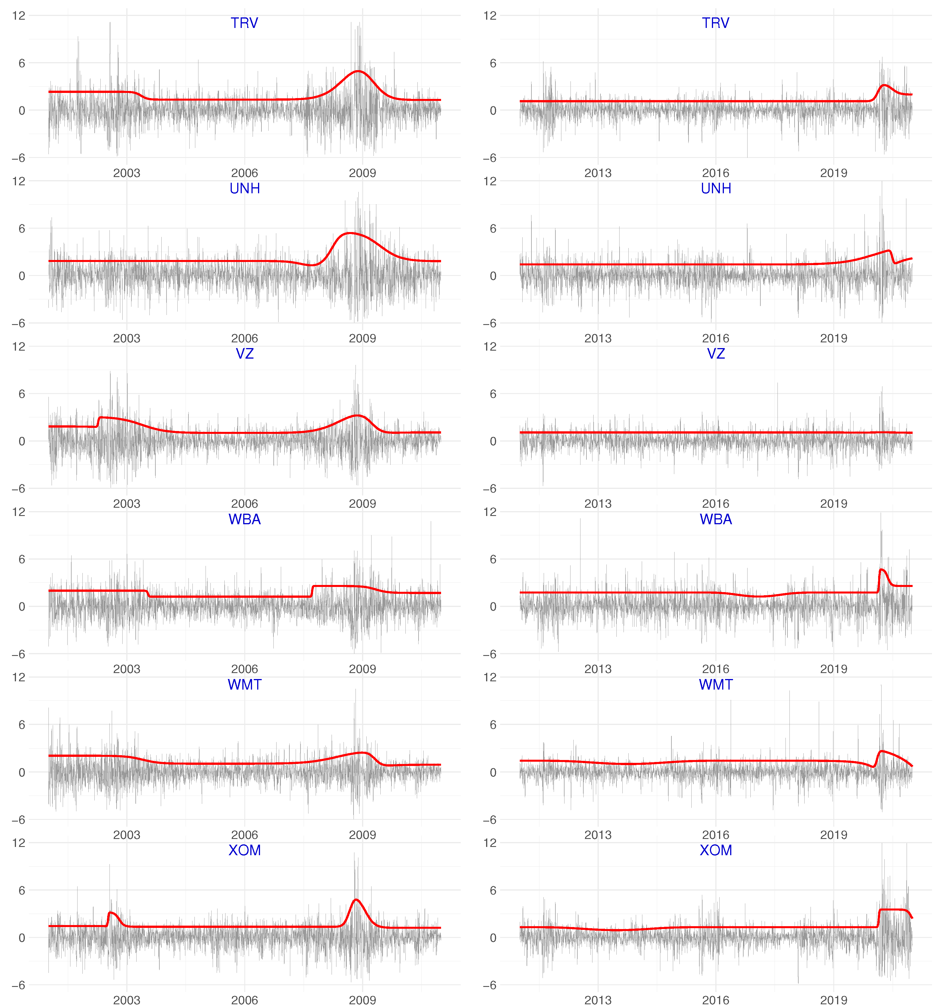
7. Application
In order to demonstrate the use of the test we select 26 stocks that have been included in the Dow Jones index during the whole observation period from 2 January 2001 to 31 December 2020 and consider their daily returns. The names, symbols and respective categories of the stocks are listed in
Table A1 in
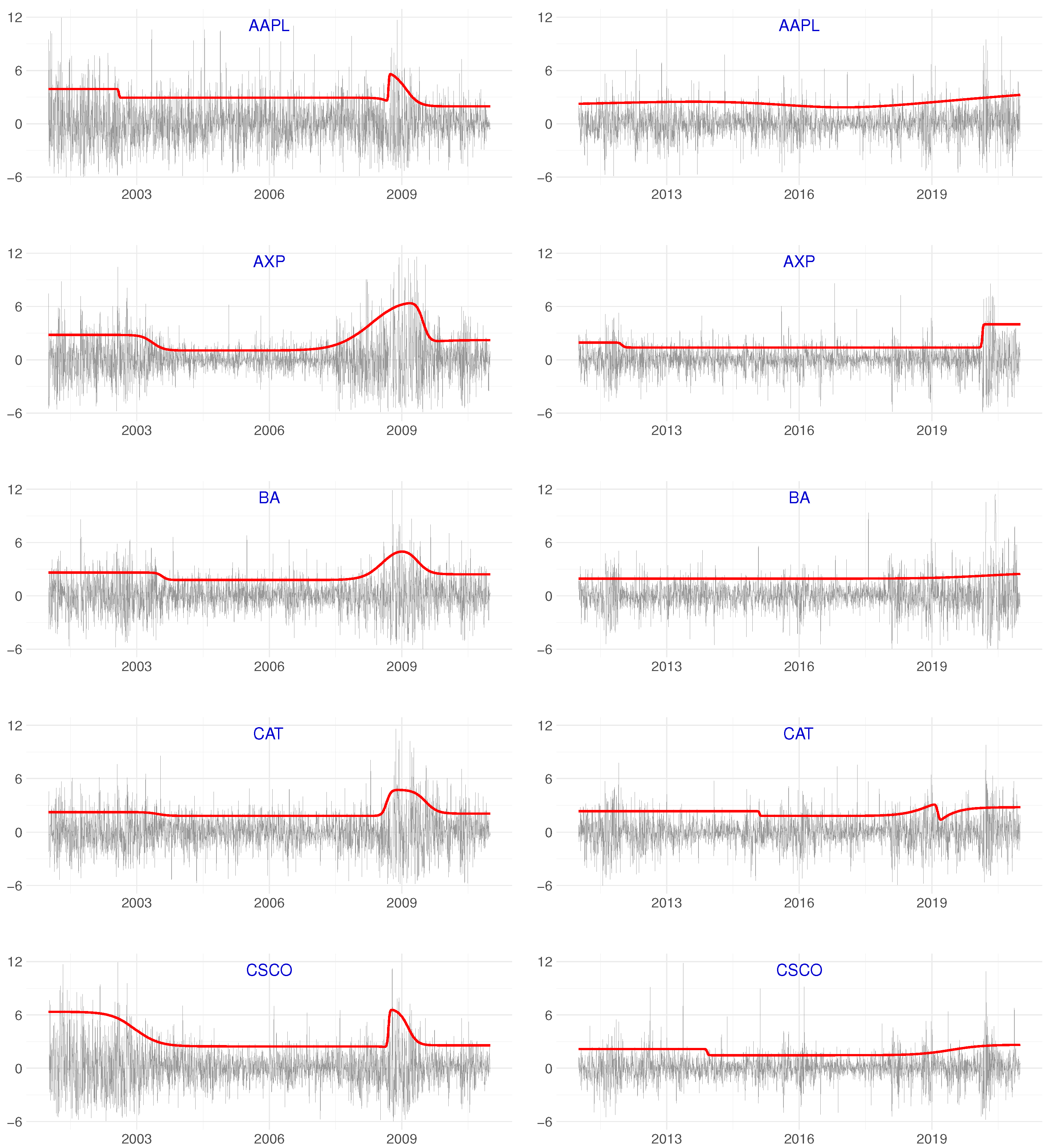
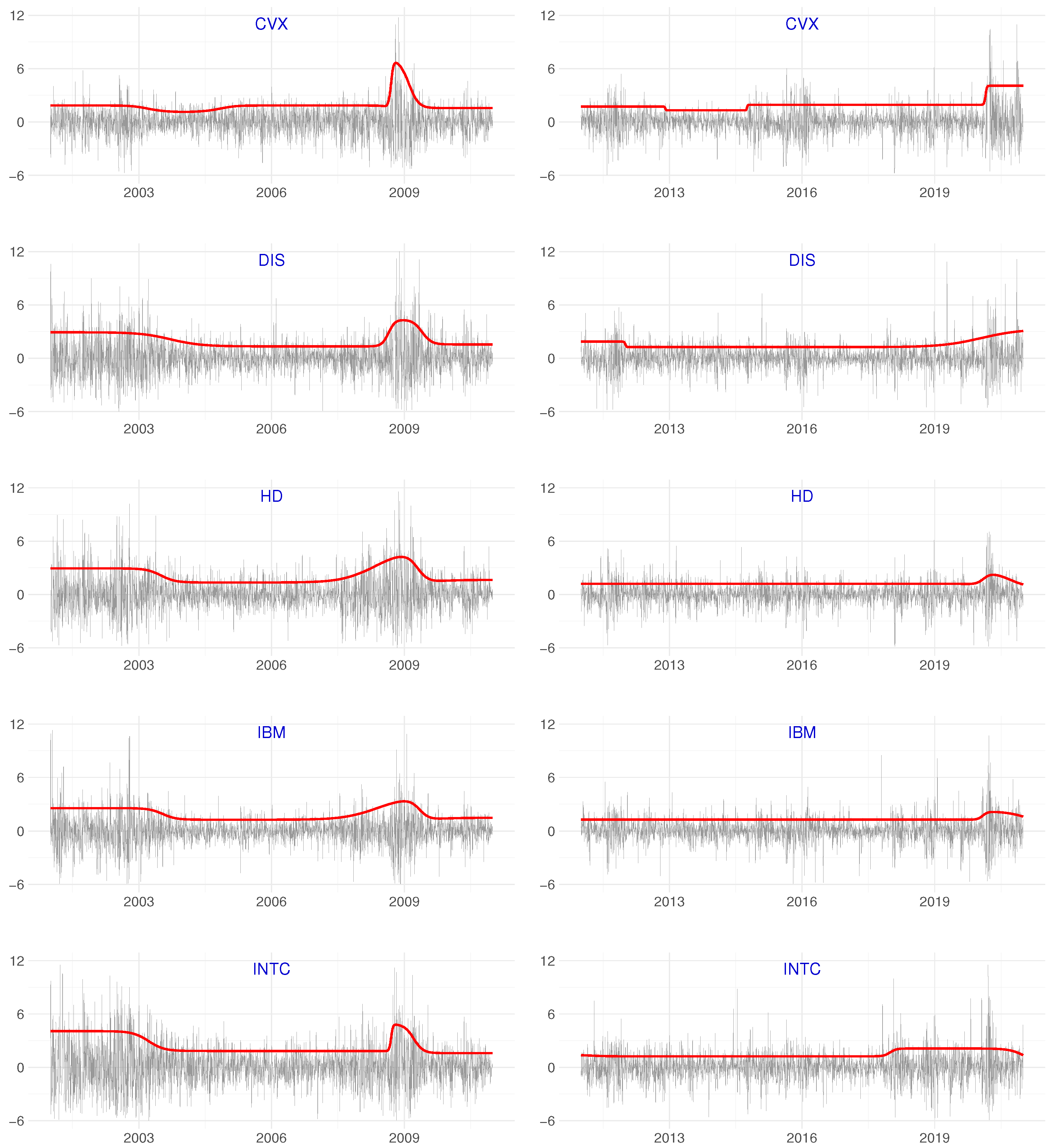
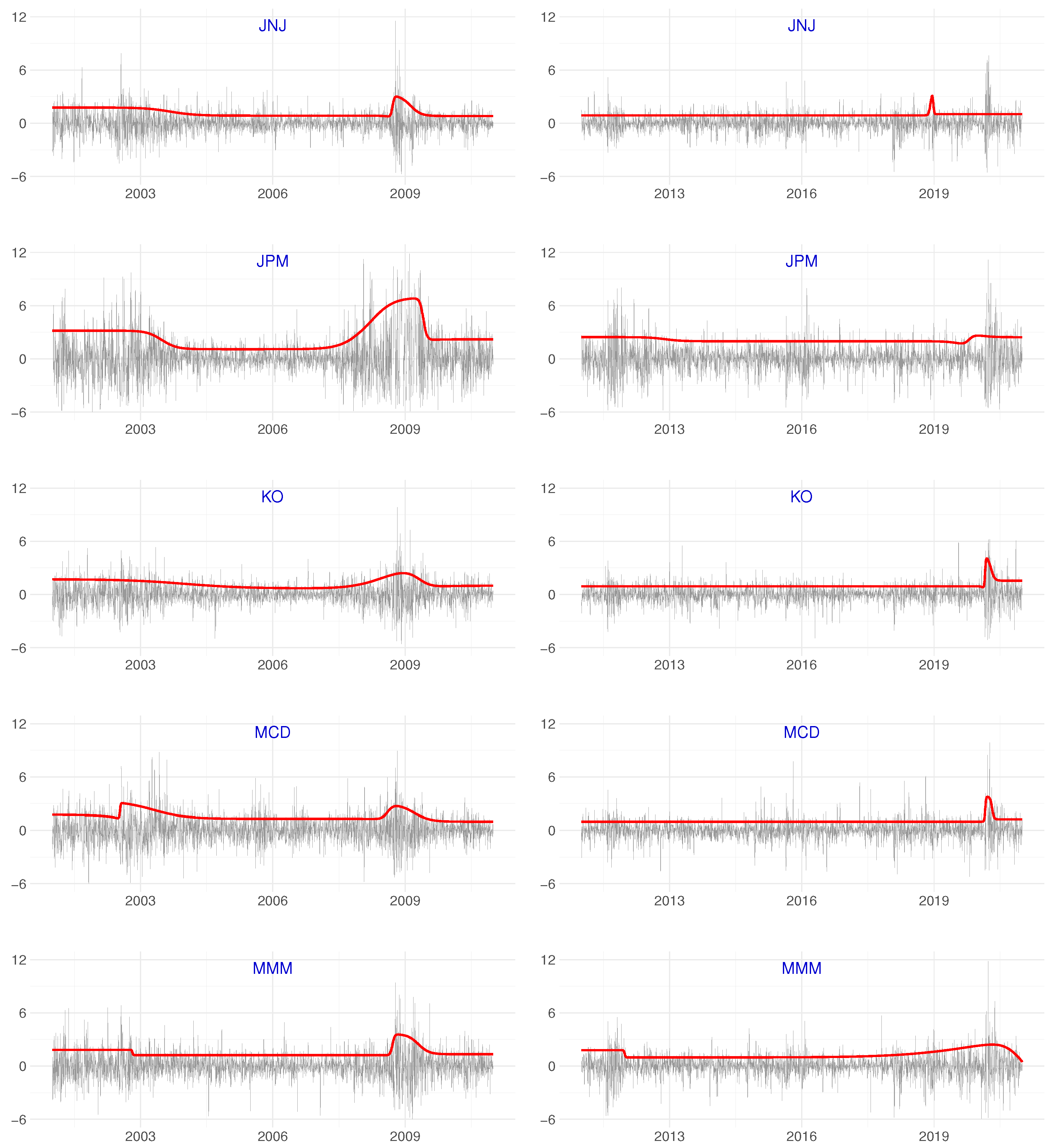
Appendix A. We split the observation period into two halves such that the returns from 2001 to the end of 2010 form the first period and the rest belong to the second one. Both samples contain approximately 2500 observations. The first part of the sample includes the periods of turbulence due to the dot-com bubble and GFC, the second is tranquil with a lead-up into the recent Covid-19 events. To perform the tests we first determine the number of transitions in the Multiplicative Time-Varying (MTV) GJR-GARCH equations (it can be zero) using the sequential procedure described in
Hall et al. (
2021). The 26 estimated GARCH equations (or their
specification test results) are not reported here, but the plots of the multiplicative component (
3) together with the daily returns appear in
Figure 6,
Figure 7,
Figure 8,
Figure 9 and
Figure 10.
The first-order test clearly rejects the null of constant correlations. Increasing the order of the polynomial in the test statistic does not affect the conclusions. Although the dimension of the null hypothesis increases from 25 to 100, all tests strongly reject the hypothesis of stable correlations for both observation periods. The p-values of the test are practically zero. If this had been attempted for the HST-test, the corresponding degrees of freedom would have increased from 325 to 1300.
While the main purpose of this example is to demonstrate the use of our tests for a relatively large set of stocks, we also consider stability of the pairwise correlations. The magnitudes of the resulting
p-values from the pairwise tests applied to the first part of the sample can be found in
Table A2 and
Table A3 for the polynomial orders of one and two, respectively.
Table A4 and
Table A5 contain the corresponding ones for the second part of the sample. In the former, the evidence of time-variation in the correlations is very clear. In the latter, there are more cases where the first-order test fails to reject constancy of correlations. The second-order test, however, does find evidence of time-varying correlations between most pairs of stocks. It appears that the change during the second period can often be nonmonotonic rather than monotonic.
This paper clearly demonstrates that our test is the most practical option when the number of assets is large. When it is small so that both tests are available, we can make comparisons and see how much power may be lost when our parsimonious test is applied instead of the HST-test. To this end, groups of three to four stocks are subsequently examined. The results are consistent in most all cases. Two exceptions are discussed next.
The four stocks representing consumer staples (WMT, WBA), services (VZ), and energy (XOM) form the first example. Our test for 2001–2010 results in p-values of 0.0134 and 0.0000 for test orders one (three degrees of freedom, df) and two (six df), respectively. In 2011–2020, the corresponding p-values are 0.1059 and 0.0001. For the HST-test, the p-values for 2001–2010 are 0.0000 for both polynomial orders (six and 12 df), and for 2011–2020 they are 0.0001 and 0.0000, respectively. The obvious conclusion is that the parsimonious test should mainly be used when the other test is no longer applicable.
The three information technology companies AAPL, IBM and INTC, form an example of the smallest collection of stocks such that our test differs from the HST-test. For 2001–2010, the
p-values for the first and second-order versions of our tests with two and four df are 0.0103 and 0.0000. The
p-values of the corresponding HST-test (three and six df) are 0.0413 and 0.0000. For the second part of the sample, the
p-values of our parsimonious test are 0.3459 and 0.0001, compared to 0.0000 for both orders for the HST-test. Here we note the rather rare occasion (2001–2010, first-order test) in which our test is more powerful than its competitor. An explanation may be found in
Table A2. It is seen that only one of the
p-values of the three pairwise tests lies below
. Thus, in the HST-test only one pair weighs towards a rejection, whereas the evidence against the null is more spread out in the test based on the eigenvalues, and the test has one df less than the HST-test.
In this example, the alternative to constancy of correlations is that the correlations vary as a function of time. However, both the parsimonious and the HST test are conditioned on the choice of the transition variable which need not be deterministic. This means that they are equally useful for practitioners who may wish to examine correlation stability over some other indicator than time. The underlying theoretical foundations of the tests are unaffected by such considerations, and hence the integrity of the tests is not compromised.


 and
and 


