Article

Estimating Directional Data From Network Topology for Improving Tracking Performance

1
COPELABS, Universidade Lusófona de Humanidades e Tecnologias, 1749-024 Lisboa, Portugal
2
UNINOVA, Monte de Caparica, 2829-516 Caparica, Portugal
3
Instituto de Telecomunicações, 1049-001 Lisboa, Portugal
4
Departamento de Engenharia Electrotécnica, Faculdade de Ciências e Tecnologia, Universidade Nova de Lisboa, 2829-516 Caparica, Portugal
*
Author to whom correspondence should be addressed.
J. Sens. Actuator Netw. 2019, 8(2), 30; https://doi.org/10.3390/jsan8020030
Submission received: 31 March 2019 / Revised: 24 April 2019 / Accepted: 13 May 2019 / Published: 20 May 2019
(This article belongs to the Special Issue Localization in Wireless Sensor Networks)

Abstract

:
This work proposes a novel approach for tracking a moving target in non-line-of-sight (NLOS) environments based on range estimates extracted from received signal strength (RSS) and time of arrival (TOA) measurements. By exploiting the known architecture of reference points to act as an improper antenna array and the range estimates, angle of arrival (AOA) of the signal emitted by the target is first estimated at each reference point. We then show how to take advantage of these angle estimates to convert the problem into a more convenient, polar space, where a linearization of the measurement models is easily achieved. The derived linear model serves as the main building block on top of which prior knowledge acquired during the movement of the target is incorporated by adapting a Kalman filter (KF). The performance of the proposed approach was assessed through computer simulations, which confirmed its effectiveness in combating the negative effect of NLOS bias and superiority in comparison with its naive counterpart, which does not take prior knowledge into consideration.

1. Introduction

Tracking a mobile target is important in many practical applications, such as autonomous surveillance, search-rescue, robotic navigation, and wildlife monitoring, to name a few [1,2,3,4,5,6,7,8,9,10,11,12,13]. Besides striving towards accurately attaining this goal, another important requirement is to do so while maintaining low implementation cost. Therefore, taking advantage of already installed technological solutions, such as terrestrial radio frequency founts, is highly supported. These include received signal strength (RSS) [14,15,16,17], time of arrival (TOA) [18,19,20,21,22], angle of arrival (AOA) [23,24,25], or perhaps an amalgamation of them [16,17,18,19,20,21,22,23,24,25,26,27,28,29,30,31,32,33,34,35,36].
Target localization and tracking problems have lured great attention in the research community lately. The authors of refs. [3,4,5,7,8,10,13,15,17,18,19,20,21,22,23,24,25,26,27,28,29,30,31,32,33,34,35,36] considered only a classical problem of target localization in wireless sensor networks (WSNs), where the authors disregarded completely any previous knowledge and awarded all significance to measurements exclusively. The authors of refs. [27,28] studied the problem of range estimation founded on RSS and TOA contents. In refs. [34,35,36], the target localization problem in a mixture of line-of-sight (LOS)/non-line-of-sight (NLOS) environments is addressed. The authors of ref. [34] started by identifying the type of path for each link based on Nakagami distribution, after which they derived a weighted least squares (WLS) estimator that makes use of TOA-only/RSS-only observations if the link is recognized as LOS/NLOS, respectively. A sequential squared range WLS estimator is presented in ref. [35]. The authors of ref. [35] partially mitigated the harmful impact of NLOS biases by managing to approximate all NLOS biases by a lone (mean) variable, after which an intermittent process was applied to obtain an estimate the location of the target. In ref. [36], the authors took into account a worst-case setting where it was assumed that every link in the network is NLOS. Founded on this, as well as the presumption that (imperfect) knowledge about the magnitude of the NLOS bias is available, they deduced a min-max problem from which a robust estimator written in a generalized trust region sub-problem structure was derived. The works in refs. [16,37,38] consider the problem of tracking a moving target, where the measurements are integrated with some previously accumulated knowledge to complement the localization precision. Nevertheless, all of these works investigate only target tracking problem based on RSS solely. The authors of ref. [14] studied the problem of tracking a moving target by incorporating hybrid, RSS and AOA, observations. The solution proposed for such a problem in ref. [14] is based on a Kalman filter (KF). For this purpose, it is assumed that sensors are equipped with suitable hardware to measure AOA. Besides the referred schemes designed particularly for RSS- and RSS-AOA-based target tracking, several other classical approaches (fundamentally nothing else but alterations of the KF) can be found in the literature nowadays. Among others, these include the extended KF (EKF) [39,40,41,42,43,44,45], which does not require any presumptions regarding the linearity of the state or measurement models. Alternatively, EKF approximates these non-linear models by the use of the first-order Taylor series expansion. Nonetheless, this implies calculating the Jacobian matrix, which can be arduous or sometimes even not feasible. Another popular modification is unscented KF, which is based on unscented transformation. This transformation is based on the rationale that it is easier to approximate a probability distribution than it is to approximate an arbitrary non-linear function or transformation [46]. The key concept here is to represent the state distribution by a least possible set of thoughtfully chosen motes, also known as sigma points. The sigma points entirely apprehend both mean and covariance of the distribution, thus, even after they are fed into the original (non-linear) model, they can still seize the mean and covariance up to the third order (Taylor series extension) for any non-linearity [46,47,48]. Analogously with the unscented KF, particle filter (PF) tends to capture the posterior probability distribution function (PDF) of the state through sample motes, referred to as particles. However, the main distinction between the two methods is that the particles are chosen randomly, and usually, high number of particles is used. Basically, a particle filter is nothing else but an ordinary randomization scheme and its performance, as well as its computational burden, highly depend on the number of particles employed [14,37]. The particles are sequentially re-sampled based on latest measurements. Similar to the previous two extensions, particle filters do not require linearity or Gaussianity presumptions [48,49]. Furthermore, the authors of refs. [1,43,50] investigated the problem of tracking a moving target with mobile sensors. Lastly, in ref. [51,52], the authors considered the target tracking problem based on fused RSS and TOA measurements. More specifically, a PF is proposed in ref. [51], whereas an EKF is presented in ref. [52].
The main contribution of this work is threefold. We show how to obtain an estimate of the AOA of the incoming radio signal without the necessity of any additional hardware, such as a directional antenna or an antenna array, which could severely raise the financial cost of the network. This is done by using range estimates extracted from RSS and TOA measurements, as well as exploiting the known topology of the available reference points to play the role of an irregular antenna array. In this way, we form triangles between a pair of anchors and the target, and use the law of cosines to estimate the angle information. Next, we also show how to make use of the estimated AOA information to effortlessly approximate the highly non-linear measurement model by a linear one. This is accomplished by applying Cartesian to polar coordinates conversion, which allows us to tackle the problem in a more suitable space given that AOA information is available. Finally, we show how to incorporate prior knowledge acquired during the target’s movement on top of the derived linear model, which results in an efficient tracking algorithm. This is achieved by applying Bayesian methodology and adapting KF equations. Hence, in huge contrast to the existing RSS and TOA tracking algorithms [51,52], the new one takes advantage of the network topology to gather extra information about the AOA of the received signal. Note that this is also in sharp contrast to the RSS-AOA tracking algorithm presented in ref. [43], where the authors assumed that anchors are conveniently equipped with additional hardware in order to measure the AOA quantity of the received signal. Moreover, instead of employing a high number of particles [51] or calculating the Jacobian matrix [52], which can considerably elevate the computational burden, the proposed approach is based on linearizing the measurement models by the use of estimated AOA information, which makes it very light in terms of computational cost.
The current work is assembled as follows. Section 2 introduces the measurement model together with the target state transition model, and formulates the target tracking problem based on a Bayesian methodology. In Section 3, the proposed technique to estimate the AOA information of the received radio signal at each anchor is described. Section 4 shows how to make use of the additional AOA information in order to linearize the measurement model on top of which prior knowledge can easily be incorporated by means of adapting KF equations. In Section 5, simulation results for a fairly complex target trajectory are presented with the objective of validating the performance of the new approach. Lastly, Section 6 abridges the main findings of the work and identifies some possible directions of our future work.

2. Problem Formulation

Let us consider a two-dimensional WSN, where a i and x t represent the known location of the ith reference point, also called anchor ( i = 1 , , N ) and the unknown location of a moving target at time t, respectively. At each time instant, the target sends a radio signal to anchors, which are adequately equipped to withdraw the RSS and the TOA quantity from the received signal. In inauspicious NLOS surroundings, RSS and TOA observations at time t, labeled as P i , t and d i , t respectively, can be modeled [27,28] as
P i , t = P 0 b i , t 10 γ log 10 x t a i d 0 + n i , t ,
d i , t = x t a i + β i , t + m i , t ,
where P 0 is the RSS (dBm) at a reference distance d 0 ( x t a i d 0 ), b i , t (dB) and β i , t (m) are the (positive) NLOS biases, γ is the path loss exponent that indicates the rate at which the RSS decreases with distance, n i , t is the log-normal shadowing term (dB) modeled as a zero-mean Gaussian random variable, i.e.,  n i , t N ( 0 , σ n i 2 ) , and  m i , t N ( 0 , σ m i 2 ) is the TOA measurement noise (m). Similar to some existing works [19,20,21], it is assumed here that the magnitude of the NLOS biases can be bounded by a known constant, i.e.,  0 b i , t b max and 0 β i , t β max . This upper bound can be easily estimated during the calibration phase [21,36].
If all RSS and all TOA observations are stored into a sole vector, i.e.,  P t = [ P i , t ] T and d t = [ d i , t ] T ( P t , d t R N ), the joint likelihood function can be written as
Λ ( P t , d t | x t , b i , t , β i , t ) = p ( P t | x t , b i , t ) p ( d t | x t , β i , t ) = 1 2 π σ n i 2 σ m i 2 exp P i , t P 0 + b i , t + 10 γ log 10 x t a i , t d 0 2 σ m i 2 + d i , t x t a i , t β i , t 2 σ n i 2 σ n i 2 σ m i 2 ,
where p ( ) denotes the probability density function (PDF). The function in Equation (2) represents the exact likelihood function if RSS and TOA measurements are taken from independent sources [28]. Even though this might not be the case in practice, the authors of refs. [27,32] showed through experimental measurements that the observations extracted from the same signal are weakly correlated.
The joint RSS-TOA maximum likelihood (ML) estimator of x t , b i , t and β i , t at time t is obtained by maximizing the joint PDF as
x t ^ , b ^ i , t , β ^ i , t = arg min x t , b i , t , β i , t i = 1 N P i , t P 0 + b i , t + 10 γ log 10 x t a i d 0 2 σ m i 2 + d i , t x t a i β i , t 2 σ n i 2 σ n i 2 σ m i 2 .
However, Equation (3) is a very difficult optimization problem that cannot be solved directly, since it is highly non-convex and under-determined (the number of unknowns, 2 N + 2 , is superior to the number of measurement readings, 2 N , at every time instant). Moreover, Equation (3) does not take any prior knowledge accumulated during the movement of the target into consideration, which, for the case of tracking a moving target, makes it a naive approach. Thus, to improve accuracy of an estimator, one should incorporate prior knowledge into the estimator.
Here, it is assumed that the target is moving according to a nearly constant velocity motion model. Therefore, the velocity elements in x- and y-directions at time t are given by
v t = v t 1 + r v , t ,
where r v , t represents the noise perturbations (e.g., due to wind gust). Therefore, according to the equations of motion [39], the location of the target at time instant t is given by
x t = x t 1 + v t 1 Δ + r x , t ,
where Δ and r x , t are, respectively, the sampling interval among two successive time steps and location process noise. Hence, by describing the target state at time instant t by both its location and velocity, that is, θ t = [ x t T , v t T ] T (i.e., θ t R 4 ), from Equations (4) and (5) it follows that
θ t = S θ t 1 + r t ,
where
S = 1 0 Δ 0 0 1 0 Δ 0 0 1 0 0 0 0 1 ,
represents the state transition matrix and r t = [ r x , t T , r v , t T ] T is the state process noise [16,37,38,42], assumed to be a zero-mean Gaussian random variable with covariance matrix Q , that is, r t N ( 0 , Q ) . This noise covariance matrix is defined by
Q = q Δ 3 3 0 Δ 2 2 0 0 Δ 3 3 0 Δ 2 2 Δ 2 2 0 Δ 0 0 Δ 2 2 0 Δ ,
where q represents the intensity of the state process noise [38,42,53]. A detailed derivation of the state transition model, as well as the matrices S and Q is given in Appendix A.
Moreover, for ease of notation, the measurement equation (Equation (1)) is rewritten in vector form as
z t = h ( x t ) + n t ,
where z t = [ P t T , d t T ] T ( z t R 2 N ) is the vector of all measurements at time instant t. Thus, the function h ( x t ) = [ h i ( x t ) ] T in Equation (7) is defined as h i ( x t ) = P 0 b i , t 10 γ log 10 x t a i d 0 for i = 1 , , N  [54], and  h i ( x t ) = x t a i + β i , t for i = N + 1 , , 2 N  [27]. The measurement noise, n t , is modeled as n t N ( 0 , C ) , with the noise covariance matrix being defined as C = diag ( [ σ n i 2 , σ m i 2 ] ) , with  diag ( ) denoting a diagonal matrix.
According to Bayesian methodology, prior knowledge, acquired via the state transition model in  Equation (6), can be combined with noisy observations in Equation (7) to get a marginal posterior PDF, p ( θ t | z 1 : t ) . The reason for this is that through p ( θ t | z 1 : t ) one can quantify the confidence one has in the values of the state θ t given all the past observations z 1 : t , from which an estimate at any desired time instant can be obtained. For the reader to have a better intuition of how it works, the key parts of the Bayesian estimation are summarized as follows [39].
  • Initialization: The marginal posterior PDF at t = 0 is set to the prior PDF p ( θ 0 ) of θ 0 .
  • Prediction: By following the state transition model in Equation (6), the predictive PDF of the state at t is given by
    p ( θ t | z 1 : t 1 ) = p ( θ t | θ t 1 ) p ( θ t 1 | z 1 : t 1 ) d θ t 1 .
  • Update: According to Bayes’ rule [42,53], one has that
    p ( θ t | z 1 : t ) = p ( z t | θ t ) p ( θ t | z 1 : t 1 ) p ( z t | z 1 : t 1 ) ,
    where p ( z t | θ t ) is the likelihood and p ( z t | z 1 : t 1 ) = p ( z t | θ t ) p ( θ t | z 1 : t 1 ) d θ t is just a normalizing constant that does not depend on θ t , required to assure that p ( θ t | z 1 : t ) integrates to 1 [39]. Generally, the marginal PDF at t 1 cannot be calculated in analytic form. Moreover, the integral in  Equation (8) cannot be obtained in closed-form, unless the state model is linear. Hence, certain approximations are necessary to get p ( θ t | z 1 : t ) .
In the following section, we show how to estimate AOA information at each anchor, by only taking advantage of the network architecture formed by anchors and range estimates from RSS and TOA measurements, without requiring any additional hardware. This information is then exploited to linearize the measurement models in Equation (1), which serve as a base on top of which we adapt a KF.

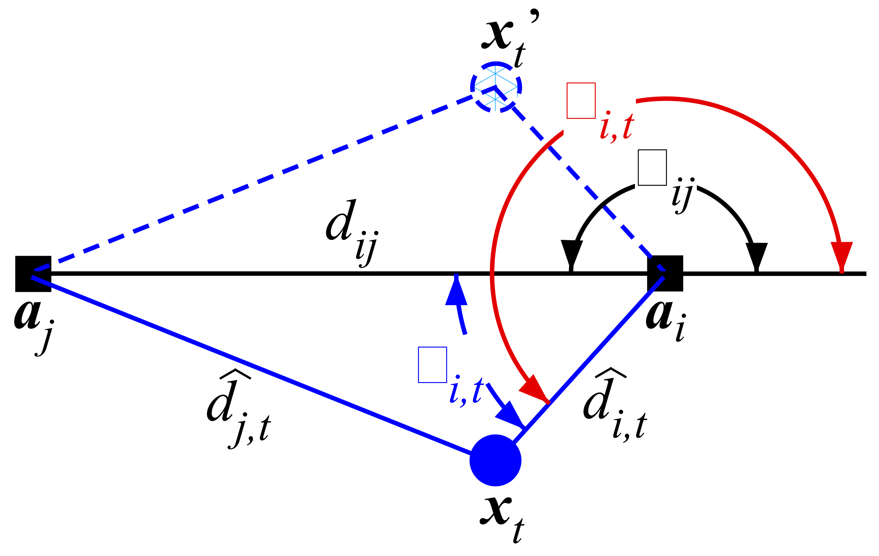
3. Angle of Arrival Estimation

Notice that, from Equation (1), the distances that best estimate x t a i in the mean ML sense are
d ^ i , t RSS = d 0 10 P 0 P i , t b max 2 10 γ ,
d ^ i , t TOA = d i , t β max 2 .
Once these distance estimates are obtained at any time instant, together with a i , i = 1 , , N , one can form triangles between any pair of anchors and the target, as illustrated in Figure 1, where d ^ i , t is used instead of d ^ i , t RSS and d ^ i , t TOA for the sake of simplicity. Hence, in each of the triangles, the lengths of the three sides are (imperfectly) known. This allows for straightforward estimation of the angle β i , t (see Figure 1), by just applying the law of cosines [55] as
β ^ i , t = cos 1 d i j 2 + d ^ i , t 2 d ^ j , t 2 2 d i j d ^ i , t ,
based on both RSS and TOA observations. Then, the estimated azimuth angle of the received radio signal at the ith anchor at time t (from both RSS and TOA measurements) is obtained according to
φ ^ i , t = α i j ± β ^ i , t ,
where α i j is the azimuth angle between anchors i and j, and ± is used due to possible orientation of the target (see Figure 1). In general, to find the right orientation of the target, i.e., the correct sign in Equation (12), it suffices to obtain only a coarse estimate of the target’s location, which, for example, can be accomplished by the trilateration approach in ref. [23]. However, due to high degree of difficulty of the problem at hand, achieving the right orientation of the target might not be feasible in practice. Therefore, due to flip-ambiguity issues, the estimation accuracy might get seriously compromised. Nonetheless, in some favorable deployments of the anchors (such as the ones considered in Section 5), where the orientation of the target is known a priori, we show that using the angle estimates in Equation (12) can significantly improve localization accuracy of an algorithm.

4. Target Tracking

In this section, we propose a novel tracking algorithm based on KF, which can be contemplated as a generalized consecutive minimum mean square estimator of a signal corrupted by noise, where the unknown parameters are permitted to develop in time in concordance with a given dynamical model [39]. What is characteristic for this filter is that, if both the state and the observation models are linear and the noise is known to be zero-mean (having finite covariance), KF renders the optimal solution in the least squares sense [42]. However, our measurement model in Equation (1) is highly non-linear. Therefore, we first take advantage of the angle estimates in Equation (12) to linearize it. This procedure allows straightforward derivation of a sub-optimal solution in a closed-form for the target localization problem in Equation (3), in which the prior knowledge is completely disregarded. Moreover, we also show that the derived linearized measurement model also triggers effortless adaptation of KF equations, which take the prior knowledge into consideration to improve the localization performance.
Note that one can rewrite Equation (10) as follows.
λ i , t x t a i = η d 0 ,
x t a i = d i , t β max 2 ,
where λ i , t = 10 P i , t + b max 2 10 γ and η = 10 P 0 10 γ . Furthermore, from geometry, one has that
φ ^ i , t = tan 1 x t y a i y x t x a i x ,
where x t y and a i y , respectively, designate the y-coordinates of the target and the ith anchor at time t, and  x t x and a i x their x-coordinates at t. By applying some simple algebraic manipulations, the above equation can be rewritten as
c i , t T x t a i = 0 ,
k i , t T x t a i = 0 ,
where c i , t = [ sin ( φ ^ i , t RSS ) , cos ( φ ^ i , t RSS ) ] T and k i , t = [ sin ( φ ^ i , t TOA ) , cos ( φ ^ i , t TOA ) ] T .
Hence, an estimate of x t can be obtained by solving the following problem
x ^ t = arg min x t i = 1 N λ i , t x t a i η d 0 2 + i = 1 N c i , t T x t a i 2 + i = 1 N x t a i d ^ i , t TOA 2 + i = 1 N k i , t T x t a i 2 ,
resulting from the application of the least squares criterion to Equations (13) and (14).
However, the problem in Equation (15) is non-convex due to the norm terms containing x t . Consequently, combating Equation (15) directly is difficult, and we take a different approach here. Rather than dealing with the problem in the Cartesian space, we exploit the estimated angles to transform Equation (15) into the polar space, a more suitable one when dealing with angles [33,56,57]. To do so, we express x t a i = r i , t u i , t in Equation (13a), with  r i , t 0 and u i , t = 1 , where the estimated unit vector is defined as u i , t = [ cos ( φ ^ i , t RSS ) , sin ( φ ^ i , t RSS ) ] T . This results in x t a i = r i , t . A similar procedure is applied to Equation (13b), where x t a i = ρ i , t v i , t , with  ρ i , t 0 and the estimated unit vector defined as v i , t = [ cos ( φ ^ i , t TOA ) , sin ( φ ^ i , t TOA ) ] T . The applied process is easily reversed by just multiplying the two equations by u i , t T u i , t = 1 , i.e.,  v i , t T v i , t = 1 , which brings us back to the Cartesian space. Thus, by enforcing the above described procedure to Equation (13), we get
λ i , t u i , t T r i , t u i , t = η d 0 λ i , t u i , t T x t a i = η d 0 ,
v i , t T ρ i , t v i , t = d ^ i , t TOA v i , t T x t a i = d ^ i , t TOA .
Consequently, Equation (16) can be rephrased in a (linear) vector form as
A t x t = b t ,
where
A t = λ 1 , t u 1 , t T λ N , t u N , t T c 1 , t T c N , t T v 1 , t T v N i , t T k 1 , t T k N , t T , b t = λ 1 , t u 1 , t T a 1 + η d 0 λ N , t u N , t T a N + η d 0 c 1 , t T a 1 c N , t T a N v 1 , t T a 1 + d ^ 1 , t TOA v N , t T a N + d ^ N , t TOA k 1 , t T a 1 k N , t T a N ,
which becomes our linearized measurement model.
With the intention to assign more belief to close by links (both RSS and TOA), we introduce weights, w t = [ w i , t ] T and ω t = [ ω i , t ] T , with  w i , t = 1 d ^ i , t R S S / i = 1 N d ^ i , t R S S and ω i , t = 1 d ^ i , t T O A / i = 1 N d ^ i , t T O A . Then, based on the WLS principle, we obtain an estimate of x t by solving
x t ^ = arg min x t i = 1 N w i , t λ i , t u i , t T x t a i η d 0 2 + i = 1 N w i , t c i , t T x t a i 2 + i = 1 N ω i , t v i , t T x t a i d ^ i , t T O A 2 + i = 1 N ω i , t k i , t T x t a i 2 .
Note that the optimization variable appears in a quadratic form in Equation (18), which makes the problem convenient to solve in closed-form. To give its solution, we first rewrite Equation (18) in a vector form as
minimize x t W t ( A t x t b t ) 2 ,
where W t = diag w t T , w t T , ω t T , ω t T , with  diag ( ) denoting a diagonal matrix. Hence, the solution to  Equation (19) is given in closed-form as
x ^ t = A t T W t T W t A t 1 A t T W t T b t .
In the remaining text, the estimator in Equation (18) is referred to as “WLS”.
Although Equation (18) is an efficient solution to the target localization problem, it completely disregards any prior knowledge one might have accumulated during the movement of the target along its trajectory. Therefore, in the following text, we show that Equation (18) can be used as the main building block on top of which prior knowledge can be incorporated.
To do so, we rely on the the most common principle of Bayesian methodology for getting a state estimate, which is the maximum a posteriori principle [39]. Based on this estimation criterion, one chooses a state estimate, θ ^ t | t , that maximizes the marginal PDF, which formally translates into
θ ^ t | t = arg max θ t p ( θ t | z 1 : t ) = arg max θ t p ( z t | θ t ) p ( θ t | z 1 : t 1 ) ,
where the second equality comes from Equation (9). By taking a closer look at Equation (20), one notices that it contains exactly what we aspired for: ML part related to the measurement model and prior PDF part related to prior knowledge. This means that, by the help of KF approach [39], we can adapt the filter’s equations to derive our own version of the KF as follows.
The mean and the covariance of the one-step predicted state are obtained according to Equation (6) as
θ ^ t | t 1 = S θ ^ t 1 | t 1
Σ ^ t | t 1 = S Σ ^ t 1 | t 1 S T + Q ,
respectively, whereas the updated mean and covariance are given by
θ ^ t | t = θ ^ t | t 1 + K t ( b ˜ t G t θ ^ t | t 1 ) ,
Σ ^ t | t = I 4 K t G t Σ ^ t | t 1 ,
with
K t = Σ ^ t | t 1 G t T ( G t Σ ^ t | t 1 G t T + C ) 1
representing the Kalman gain at time instant t, and  G t = [ A t , 0 2 N × 2 ] ( G t R 2 N × 4 ).
A step-by-step framework of the proposed KF algorithm (labeled here as “KF”) is summarized in Algorithm 1, and its flow chart is illustrated in Figure 2.
Algorithm 1 KF algorithm description.
Require: S , Q , C , z t , for  t = 0 , , T
1:
Initialization: x ^ 0 | 0 E q u a t i o n ( 19 ) , θ ^ 0 | 0 [ x ^ 0 | 0 T , 0 , 0 ] T , Σ ^ 0 | 0 I 4
2:
for t = 1 , , T do
3:
Prediction:
  • θ ^ t | t 1 Equation ( 21 a )
  • Σ ^ t | t 1 Equation ( 21 b )
4:
Kalman gain:
  • K t Equation ( 23 )
5:
Update:
  • θ ^ t | t Equation ( 22 a )
  • Σ ^ t | t Equation ( 22 b )
6:
end for

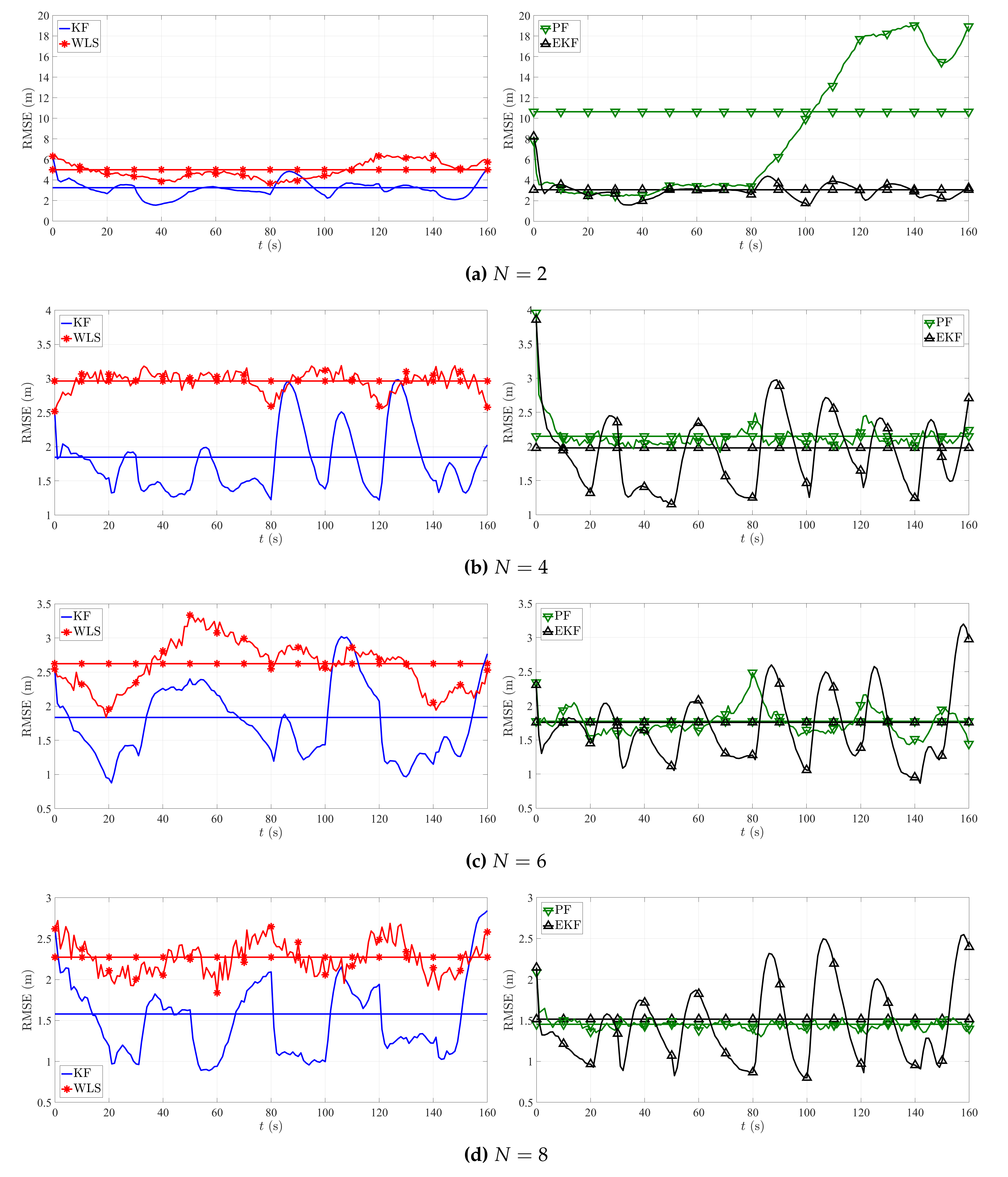
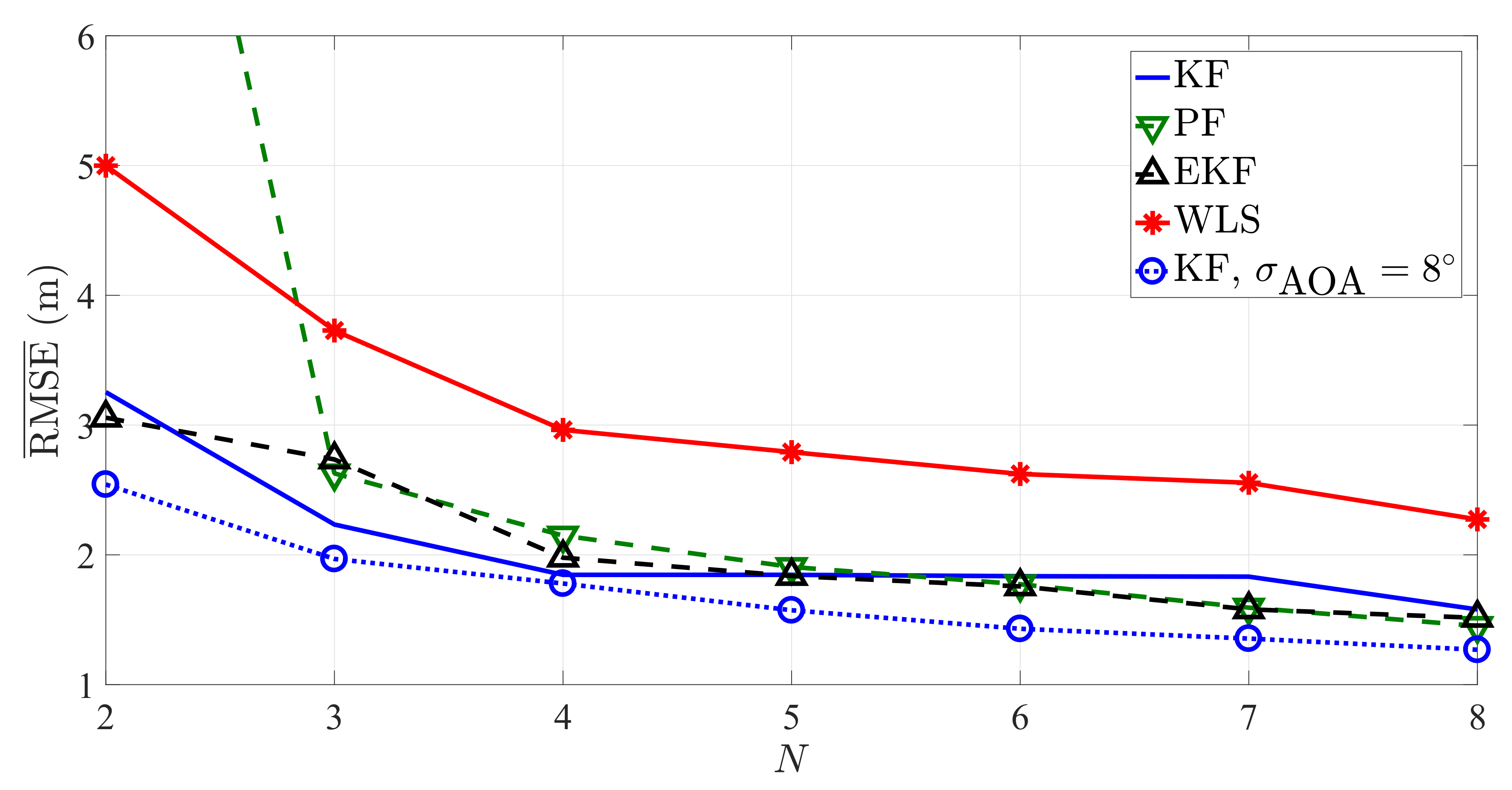
5. Performance Results

This section validates the performance of the proposed algorithm based on computer simulations. The considered algorithms, the PF in ref. [51] and the EKF in ref. [52], as well as the WLS in Equation (19) and the proposed KF in Algorithm 1, were implemented in MATLAB, and the radio measurements were generated according to Equation (1). True anchor locations are summarized in Table 1, whereas the target follows the trajectory illustrated in Figure 3 within an area of B × B m 2 in every Monte Carlo, M c , run. The rest of the simulation parameters are summarized in Table 2. Furthermore, NLOS biases (both b i (dB) and β i (m), jointly designated here as bias i for simplicity) are generated randomly from a uniform distribution on the interval [ 0 , bias max ] (dB, m), i.e., bias i U [ 0 , bias max ] , i = 1 , , N in each M c run. The main performance metric is the root mean squared error (RMSE), RMSE = i = 1 M c x i , t x ^ i , t M c , where x ^ i , t denotes the estimate of the true target location, x i , t , in the ith M c run at time instant t.
The proposed KF algorithm is compared with the existing RSS and TOA tracking algorithms, namely the PF in ref. [51] and the EKF in ref. [52], as well as the WLS in Equation (19), which represents its main building block that disregards the prior knowledge, in the scenario illustrated in Figure 3. Note that the trajectory in Figure 3 is composed of several straight-line trajectories connected by sharp maneuvers, together with somewhat smoother maneuvers, but with constant changes in the direction of movement; hence, it represents a fairly complex trajectory, whose portions are often found in practice. Moreover, notice that a constant speed of the target is considered here for simplicity. This does not cause loss of generality, since the proposed KF algorithm is extremely light in terms of computational cost, which translates into its execution time being of order of milliseconds. In other words, this means that we could drastically reduce the sampling interval, which would result in much smaller steps of the target (at the order of centimeters) within a sample period, producing the effect of approximately constant velocity model for virtually all achievable speeds in practice. Lastly, to conclude the simulation setting part, it is worth mentioning that, in all simulations presented here, the first N anchors from Table 1 were used.
Figure 4 plots a realization of the estimation trial in the considered setting of KF and WLS in a single M c run. On the one hand, the figure clearly shows that KF has much smoother performance and traces the target’s trajectory more accurately. Naturally, KF struggles slightly at each sharp maneuver of the target. This is explained by the fact that at these points all previously acquired prior knowledge becomes fallacious, and misleads KF to stumble. Nevertheless, it can be seen that KF recovers quite quickly from these predicaments. On the other hand, the figure shows that, although the performance of WLS does not suffer such inconveniences and is fairly good, the trace of the trajectory obtained through WLS seems a bit chaotic. This is because WLS disregards the prior knowledge, and every plotted estimation point is a result independent of any previous one.
Figure 5 illustrates the RMSE (m) versus t performance for various N. Besides the RMSE at each time instant t, the average RMSE, RMSE ¯ , for all t is also shown in the figure (straight horizontal lines marked with respective symbols and colors). Superior performance of tracking algorithms is clearly noted in general. Interestingly, the tracking algorithms are not always better than WLS, i.e., not at all time instants. It seems that KF and EKF struggle with the sharp maneuvers taken by the target at the top right corner of its trajectory and the one immediately after. Nevertheless, these peaks in the performance of KF and EKF are of relatively short duration, and do not change the overall conclusion that incorporating prior knowledge can improve the performance of an algorithm. Finally, it can be seen from the figure that, apart from the case where N = 2 , PF has the most stable performance, with very few peaks. This is not too surprising, since its performance is directly proportional to the number of particles used, but so is its computational complexity.
Figure 6 illustrates RMSE ¯ (m) versus N performance. In addition to KF, PF, EKF and WLS algorithms, we also include the results for the counterpart of the proposed KF, when, instead of estimating the angles, anchors can measure them. These results can be seen as a lower bound on the performance of the new algorithm. Nonetheless, it is worth noting that, in order for these results to be feasible, anchors would require additional hardware, such as a directional antenna or an antenna array, which would raise the network implementation cost. Moreover, the angle measurement noise power was drawn from a zero-mean von Mises distribution [56] with the concentration parameter set as to correspond to a zero-mean Normal distribution with noise power σ AOA = 8 , as stated explicitly in Figure 6. The figure exhibits that the performance of all algorithms betters when N is increased. This behavior is anticipated, due to extra information gathered within the network with every additional anchor. Furthermore, apart from the performance of PF for N = 2 , the performance of the tracking algorithms is superior than that of WLS for all N, with the biggest margin for low N, which confirms the hypothesis that prior knowledge can be exploited to improve localization accuracy. Finally, one can notice that the performance of the proposed KF is fairly close to its counterpart that can measure the AOA. This is an important result, which suggests that the proposed approach for angle estimation is a useful one in practical scenarios where no additional hardware to measure the AOA is available.
Figure 7 illustrates RMSE ¯ (m) versus noise powers, σ i (dB, m), performance comparison. To get a better comprehension of the influence of this parameter on localization performance, the magnitude of the NLOS bias was set to a relatively small value, i.e., bias max = 1 (dB, m) was considered. Naturally, when the measurement quality deteriorates, i.e., when σ i (dB, m) grows, the localization accuracy drops. Nevertheless, Figure 7 shows that KF has superior performance in noisy environments, outperforming significantly WLS (almost 2.5 m) and PF and EKF (roughly 1 m). This result confirms that our linearization technique is a well-founded solution, since our derivation do not make any assumptions about noise levels.
Figure 8 illustrates RMSE ¯ (m) versus bias max (dB, m) performance comparison. Similar to the previous setting, to better see the influence of this parameter on the performance of the considered algorithm, the noise powers were set to a relatively small value, i.e., σ i = 1 (dB, m) was considered. As before, Figure 8 corroborates the superiority of tracking algorithms over classical localization ones for all considered values of bias max (dB, m), indicating that prior knowledge should not be disregarded. However, achieving precision just above 3 m for WLS suggests that the proposed approach handles NLOS bias efficiently, even for a naive approach.

6. Conclusions and Future Work

In this work, we proposed a novel approach for tracking a moving target in adverse NLOS environments by means of combined RSS and TOA measurements. Initially, we showed how to estimate the angle of the received signal at each reference point, without requiring any additional hardware. For this purpose, the known topology of the reference points was exploited to act as an irregular antenna array, which together with range estimates obtained through RSS and TOA measurements allowed us to form triangles with (imperfectly) known side lengths between a pair of reference points and the target. From there, we simply applied the law of cosines to get the desired AOA estimations. We then showed how to use these estimates to effortlessly convert the originally non-linear measurement model into a linear one, by applying Cartesian to polar coordinates transformation. On top of the linearized model, we incorporated prior knowledge acquired during the movement of the target, by adaptation of the KF equations. The proposed approach was assessed via computer simulations in which a fairly complex target trajectory was studied. In all considered scenarios, the new approach exhibited good performance, corroborating our intuition that one can benefit from extra information inherent in the network topology.
Note that the proposed approach is not restricted to RSS and/or TOA measurements, but can easily be adapted to any range-based localization/tracking technique, as it merely requires distance information and a couple of reference point. Even though we showed here that it can be very beneficial for the problem at hand, some challenges remain. For instance, the application of the proposed approach to an ad-hoc network is straightforward, but one has to be able to resolve the problem of target orientation, i.e., flip-ambiguity. This is very demanding to achieve always due to elevated degree of difficulty of the considered problem (NLOS bias, noise, etc.), which obviously reflects on the estimation accuracy. Therefore, our future research will include combating flip-ambiguity in order to accomplish also full potential of the proposed approach in ad-hoc networks. In addition, testing the proposed KF algorithm against real-world experimental measurements will be of highest priority.

Author Contributions

Formal analysis, S.T., M.B., R.D. and P.M.; writing—original draft preparation, S.T., M.B., R.D. and P.M.; and writing—review and editing, S.T., M.B., R.D. and P.M. All authors contributed equally to this work.

Funding

This work was partially supported by Fundação para a Ciência e a Tecnologia under Projects UID/MULTI/04111/0213 and UID/MULTI/04111/0216 (COPELABS—Cognitive and People-centric computing), UID/EEA/00066/2013 and foRESTER PCIF/SSI/0102/2017, UID/EEA/50008/2019, PES3N POCI-01-0145- FEDER-030629 and Grant IF/00325/2015.

Conflicts of Interest

The authors declare no conflict of interest.

Appendix A. Derivation of the State Transition Model

Consider the following continuous-time state transition model [58].
θ ˙ ( t ) = A θ ( t ) + D u ( t ) + B r ( t ) , θ ( t 0 ) = θ 0 ,
where θ ( t ) R n is the state vector; u ( t ) R p is the vector containing any control inputs (steering angle, throttle setting, and breaking force); A R n × n , D R n × p and B R n × r are the transition, input gain and noise gain matrices, respectively; and r ( t ) is a continuous-time process noise with covariance Q ( t ) .
By using Euler’s method or zero-order hold [59,60], we can rewrite the continuous-time state transition model in Equation (A1) for a time-invariant continuous-time system with sampling rate Δ , for initial time t 0 = t Δ and final time t f = ( t + 1 ) Δ , as
θ ( t f ) = exp A ( t f t 0 ) θ ( t 0 ) + t 0 t f exp A ( t f τ ) D u ( τ ) + B r ( τ ) d τ ,
which is equivalent to
θ ( t + 1 ) = exp A Δ θ ( t ) + t Δ ( t + 1 ) Δ exp A ( ( t + 1 ) Δ τ ) D u ( τ ) + B r ( τ ) d τ .
If we assume that the input u ( t ) changes slowly, relative to the sampling period, we have u ( t f ) u ( t 0 ) for t 0 t t f . Then, by changing the variable of integration φ = ( t + 1 ) Δ τ such that d φ = d τ , Equation (A2) can be rewritten
θ ( t + 1 ) = exp A Δ θ ( t ) + Δ 0 exp A φ D ( d φ ) u ( t ) + t Δ ( t + 1 ) Δ exp A ( ( t + 1 ) Δ τ ) B r ( τ ) d τ = exp A Δ θ ( t ) + 0 Δ exp A φ D d φ u ( t ) + t Δ ( t + 1 ) Δ exp A ( ( t + 1 ) Δ τ ) B r ( τ ) d τ ,
and the state model in Equation (A1) can be discretized as
θ t + 1 = S θ t + G u t + r t ,
where
S = exp A Δ ,
G = 0 Δ exp A φ D d φ ,
r t = t Δ ( t + 1 ) Δ exp A ( ( t + 1 ) Δ τ ) B r ( τ ) d τ .
The process noise, r ( t ) , is assumed to be zero-mean and white Gaussian, and the discretized process noise, r t , retains the same characteristics [58], i.e.,
E r t = 0 , E r t r t T = Q t δ t ,
where δ t represents a Dirac impulse, and the covariance of the state process noise is given, according to Equation (A5), as
Q t = 0 Δ exp A ( ( t + 1 ) Δ τ ) B Q B T exp A T ( ( t + 1 ) Δ τ ) d τ ,
and Q = diag ( [ q , q ] ) , with q denoting a tuning parameter for the state process noise intensity.
Since this thesis assumes a two-dimensional constant velocity model, the continuous-time target state model in Equation (A1) can be simplified [58] as
θ ˙ ( t ) = A θ ( t ) + B r ( t ) ,
where
A = 0 0 1 0 0 0 0 1 0 0 0 0 0 0 0 0 , B = 0 0 0 0 1 0 0 1 ,
and r ( t ) N ( 0 , Q ) .
The discrete-time model equivalent to the above one is described by
θ t + 1 = S θ t + r t ,
where, by solving Equations (A4) and (A6), respectively, we get
S = 1 0 Δ 0 0 1 0 Δ 0 0 1 0 0 0 0 1 , Q = q Δ 3 3 0 Δ 2 2 0 0 Δ 3 3 0 Δ 2 2 Δ 2 2 0 Δ 0 0 Δ 2 2 0 Δ .

References

  1. Xu, E.; Ding, Z.; Dasgupta, S. Target Tracking and Mobile Sensor Navigation in Wireless Sensor Networks. IEEE Trans. Mob. Comput. 2013, 12, 177–186. [Google Scholar] [CrossRef]
  2. Tomic, S.; Beko, M.; Dinis, R.; Tuba, M.; Bacanin, N. RSS-AoA-Based Target Localization and Tracking in Wireless Sensor Networks, 1st ed.; River Publishers: Delft, The Netherlands, 2017. [Google Scholar]
  3. Correia, S.; Beko, M.; Cruz, L.; Tomic, S. Elephant Herding Optimization for Energy-Based Localization. Sensors 2019, 18, 2849. [Google Scholar]
  4. Chalisea, B.K.; Zhanga, Y.D.; Amina, M.G.; Himed, B. Target Localization in a Multi-static Passive Radar System Through Convex Optimization. Signal Process. 2014, 102, 207–215. [Google Scholar] [CrossRef]
  5. Tomic, S.; Beko, M. Target Localization via Integrated and Segregated Ranging Based on RSS and TOA Measurements. Sensors 2019, 19, 230. [Google Scholar]
  6. Martínez, S.; Bullo, F. Optimal Sensor Placement and Motion Coordination for Target Tracking. Automatica 2006, 42, 661–668. [Google Scholar] [CrossRef]
  7. Beko, M. Energy-based Localization in Wireless Sensor Networks Using Second-order Cone Programming Relaxation. Wirel. Pers. Commun. 2014, 77, 1847–1857. [Google Scholar]
  8. Pedro, D.; Tomic, S.; Bernardo, L.; Beko, M.; Oliveira, R.; Dinis, R.; Pinto, P.; Amaral, P. Algorithms for Estimating the Location of Remote Nodes Using Smartphones. IEEE Access 2019. [Google Scholar] [CrossRef]
  9. Paz, L.M.; Tardós, J.D.; Neira, J. Divide and Conquer: EKF SLAM in 𝒪(n). IEEE Trans. Robot. 2008, 24, 1107–1120. [Google Scholar] [CrossRef]
  10. Tomic, S.; Beko, M.; Dinis, R.; Bernardo, L. On Target Localization Using Combined RSS and AoA Measurements. Sensors 2018, 18, 1266. [Google Scholar] [CrossRef]
  11. Ding, Y.; Zhu, M.; He, Y.; Jiang, J. P-cmommt Algorithm for the Cooperative Multi-robot Observation of Multiple Moving Targets. In Proceedings of the 2006 6th World Congress on Intelligent Control and Automation, Dalian, China, 21–23 June 2006; pp. 661–668. [Google Scholar]
  12. Tomic, S.; Beko, M. Exact Robust Solution to TW-ToA-based Target Localization Problem with Clock Imperfections. IEEE Sign. Process. Lett. 2018, 25, 531–535. [Google Scholar] [CrossRef]
  13. Patwari, N.; Ash, J.N.; Kyperountas, S.; Moses, R.L.; Correal, N.S. Locating the Nodes: Cooperative Localization in Wireless Sensor Networks. IEEE Sign. Process. Mag. 2005, 22, 54–69. [Google Scholar] [CrossRef]
  14. Khan, M.W.; Kemp, A.H.; Salman, N.; Mihaylova, L.S. Tracking of Wireless Mobile Nodes in the Presence of Unknown Path-loss Characteristics. In Proceedings of the 2015 18th International Conference on Information Fusion (Fusion), Washington, DC, USA, 6–9 July 2015; pp. 104–111. [Google Scholar]
  15. Tomic, S.; Beko, M.; Dinis, R. Distributed RSS-Based Localization in Wireless Sensor Networks Based on Second-Order Cone Programming. Sensors 2014, 14, 18410–18432. [Google Scholar] [CrossRef] [PubMed]
  16. Khan, M.W.; Salman, N.; Ali, A.; Khan, A.M.; Kemp, A.H. A Comparative Study of Target Tracking With Kalman Filter, Extended Kalman Filter and Particle Filter Using Received Signal Strength Measurements. In Proceedings of the 2015 International Conference on Emerging Technologies (ICET), Peshawar, Pakistan, 19–20 December 2015; pp. 1–6. [Google Scholar]
  17. Tomic, S.; Beko, M.; Dinis, R. RSS-based Localization in Wireless Sensor Networks Using Convex Relaxation: Noncooperative and Cooperative Schemes. IEEE Trans. Veh. Technol. 2015, 64, 2037–2050. [Google Scholar] [CrossRef]
  18. Qua, X.; Xie, L. An Efficient Convex Constrained Weighted Least Squares Source Localization Algorithm Based on TDOA Measurements. Signal Process. 2016, 119, 142–152. [Google Scholar] [CrossRef]
  19. Wang, G.; Chen, H.; Li, Y.; Ansari, N. NLOS Error Mitigation for TOA-Based Localization via Convex Relaxation. IEEE Trans. Wirel. Commun. 2014, 13, 4119–4131. [Google Scholar] [CrossRef]
  20. Tomic, S.; Beko, M.; Dinis, R.; Montezuma, P. A Robust Bisection-based Estimator for TOA-based Target Localization in NLOS Environments. IEEE Commun. Lett. 2017, 21, 2488–2491. [Google Scholar] [CrossRef]
  21. Zhang, S.; Gao, S.; Wang, G.; Li, Y. Robust NLOS Error Mitigation Method for TOA-Based Localization via Second-Order Cone Relaxation. IEEE Commun. Lett. 2015, 19, 2210–2213. [Google Scholar] [CrossRef]
  22. Tomic, S.; Beko, M. A Bisection-based Approach for Exact Target Localization in NLOS Environments. Sign. Process. 2018, 143, 328–335. [Google Scholar] [CrossRef]
  23. Niculescu, D.; Nath, B. Ad Hoc Positioning System (APS) Using AoA. In Proceedings of the Twenty-second Annual Joint Conference of the IEEE Computer and Communications Societies, San Francisco, CA, USA, 30 March–3 April 2003. [Google Scholar]
  24. Yu, K. 3-D Localization Error Analysis in Wireless Networks. IEEE Trans. Wirel. Commun. 2007, 6, 3473–3481. [Google Scholar]
  25. Biswas, P.; Aghajan, H.; Ye, Y. Semidefinite Programming Algorithms for Sensor Network Localization Using Angle of Arrival Information. In Proceedings of the Thirty-Ninth Asilomar Conference on Signals, Systems and Computers, Pacific Grove, CA, USA, 30 October–2 November 2005; pp. 220–224. [Google Scholar]
  26. Tomic, S.; Beko, M.; Dinis, R. 3-D Target Localization in Wireless Sensor Network Using RSS and AoA Measurement. IEEE Trans. Vehic. Technol. 2017, 66, 3197–3210. [Google Scholar] [CrossRef]
  27. Zhang, J.; Ding, L.; Wang, Y.; Hu, L. Measurement-based Indoor NLOS TOA/RSS Range Error Modelling. Electron. Lett. 2016, 52, 165–167. [Google Scholar] [CrossRef]
  28. Coluccia, A.; Fascista, A. On the Hybrid TOA/RSS Range Estimation in Wireless Sensor Networks. IEEE Trans. Wirel. Commun. 2018, 17, 361–371. [Google Scholar] [CrossRef]
  29. Tomic, S.; Beko, M.; Dinis, R. Distributed RSS-AoA Based Localization with Unknown Transmit Powers. IEEE Wirel. Commun. Lett. 2016, 5, 392–395. [Google Scholar] [CrossRef]
  30. Yin, J.; Wan, Q.; Yang, S.; Ho, K.C. A Simple and Accurate TDOA-AOA Localization Method Using Two Stations. IEEE Sign. Process. Lett. 2016, 23, 144–148. [Google Scholar] [CrossRef]
  31. Tomic, S.; Beko, M.; Dinis, R.; Montezuma, P. Distributed Algorithm for Target Localization in Wireless Sensor Networks Using RSS and AoA Measurements. Pervasive Mob. Comput. 2017, 37, 63–77. [Google Scholar] [CrossRef]
  32. Macii, D.; Colombo, A.; Pivato, P.; Fontanelli, D. A Data Fusion Technique for Wireless Ranging Performance Improvement. IEEE Trans. Indstr. Meas. 2013, 62, 27–37. [Google Scholar] [CrossRef]
  33. Tomic, S.; Beko, M.; Dinis, R.; Montezuma, P. A Closed-form Solution for RSS/AoA Target Localization by Spherical Coordinates Conversion. IEEE Wirel. Commun. Lett. 2016, 5, 680–683. [Google Scholar] [CrossRef]
  34. Tiwari, S.; Wang, D.; Fattouche, M.; Ghannouchi, F. A Hybrid RSS/TOA Method for 3D Positioning in an Indoor Environment. ISRN Sign. Process. 2012, 2012, 503707. [Google Scholar] [CrossRef]
  35. Tomic, S.; Beko, M.; Tuba, M.; Correia, V.M.F. Target Localization in NLOS Environments Using RSS and TOA Measurements. IEEE Wirel. Commun. Lett. 2018, 7, 1062–1065. [Google Scholar] [CrossRef]
  36. Tomic, S.; Beko, M.; Tuba, M.; Correia, V.M.F. Target Localization in NLOS Environments Using RSS and TOA Measurements. IEEE Sign. Process. Lett. 2019, 26, 64–68. [Google Scholar] [CrossRef]
  37. Beaudeau, J.P.; Bugallo, M.F.; Djuric, P.M. RSSI-based Multi-target Tracking by Cooperative Agents Using Fusion of Cross-target Information. IEEE Trans. Sign. Process. 2015, 63, 5033–5044. [Google Scholar] [CrossRef]
  38. Masazade, E.; Niu, R.; Varshney, P.K. Dynamic Bit Allocation for Object Tracking in Wireless Sensor Networks. IEEE Trans. Sign. Process. 2012, 60, 5048–5063. [Google Scholar] [CrossRef]
  39. Kay, S.M. Fundamentals of Statistical Signal Processing: Estimation Theory; Prentice-Hall: Upper Saddle River, NJ, USA, 1993. [Google Scholar]
  40. Tomic, S.; Beko, M.; Dinis, R.; Tuba, M.; Bacanin, N. Bayesian Methodology for Target Tracking Using RSS and AoA Measurements. Phys. Commun. 2017, 25, 158–166. [Google Scholar] [CrossRef]
  41. Bar-Shalom, Y.; Fortmann, T.E. Tracking and Data Association; Academic Press Professional, Inc.: San Diego, CA, USA, 1987. [Google Scholar]
  42. Dardari, D.; Closas, P.; Djuric, P.M. Indoor Tracking: Theory, Methods, and Technologies. IEEE Trans. Vehic. Technol. 2016, 64, 1263–1278. [Google Scholar] [CrossRef]
  43. Tomic, S.; Beko, M.; Dinis, R.; Gomes, J.P. Target Tracking with Sensor Navigation Using Coupled RSS and AoA Measurements. Sensors 2017, 17, 2690. [Google Scholar] [CrossRef]
  44. Zhao, Z.; Chen, H.; Chen, G.; Kwan, C.; Li, X.R. Comparison of Several Ballistic Target Tracking Filters. In Proceedings of the 2006 American Control Conference, Minneapolis, MN, USA, 14–16 June 2006; pp. 2197–2202. [Google Scholar]
  45. Farina, A.; Ristic, B.; Benvenuti, D. Tracking a Ballistic Target: Comparison of Several Nonlinear Filters. IEEE Trans. Aerosp. Electron. Syst. 2002, 38, 854–867. [Google Scholar] [CrossRef]
  46. Julier, S.J.; Uhlmann, J.K. Unscented Filtering and Nonlinear Estimation. Proc. IEEE 2004, 92, 401–422. [Google Scholar] [CrossRef]
  47. Wan, E.A.; van der Merwe, R. The Unscented Kalman Filter for Nonlinear Estimation. In Proceedings of the IEEE 2000 Adaptive Systems for Signal Processing ommunications, and Control Symposium, Lake Louise, AB, Canada, 4 October 2000; pp. 1–6. [Google Scholar]
  48. Chatzi, E.N.; Smyth, A.W. The Unscented Kalman Filter and Particle Filter Methods for Nonlinear Structural System Identification with Non-collocated Heterogeneous Sensing. Struct. Control Health Monit. 2009, 16, 99–123. [Google Scholar] [CrossRef]
  49. Chen, Z. Bayesian Filtering: From Kalman Filters to Particle Filters, and Beyond. Statistics 2003, 182, 1–69. [Google Scholar] [CrossRef]
  50. Zou, Y.; Chakrabarty, K. Distributed Mobility Management for Target Tracking in Mobile Sensor Networks. IEEE Trans. Mob. Comput. 2007, 6, 872–887. [Google Scholar] [CrossRef]
  51. Song, Y.; Yu, H. A New Hybrid TOA/RSS Location Tracking Algorithm for Wireless Sensor Network. In Proceedings of the 2008 9th International Conference on Signal Processing, Beijing, China, 26–29 December 2008; pp. 2645–2648. [Google Scholar]
  52. Khan, R.; Sottile, F.; Spirito, M.A. Hybrid Positioning through Extended Kalman Filter with Inertial Data Fusion. IJIEE 2013, 3, 127–131. [Google Scholar]
  53. Wang, G.; Li, Y.; Jin, M. On MAP-based Target Tracking Using Range-only Measurements. In Proceedings of the 2013 8th International Conference on Communications and Networking in China (CHINACOM), Guilin, China, 14–16 August 2013; pp. 1–6. [Google Scholar]
  54. Rappaport, T.S. Wireless Communications: Principles and Practice; Prentice-Hall: Upper Saddle River, NJ, USA, 1996. [Google Scholar]
  55. Kannan, A.A.; Fidan, B.; Mao, G.; Anderson, B.D.O. Analysis of Flip Ambiguities in Distributed Network Localization. In Proceedings of the 2007 Information, Decision and Control, Adelaide, Australia, 12–14 February 2017; pp. 193–198. [Google Scholar]
  56. Mardia, K.V. Statistics of Directional Data; Academic Press, Inc.: London, UK, 1972. [Google Scholar]
  57. Tomic, S.; Beko, M.; Tuba, M. A Linear Estimator for Network Localization Using Integrated RSS and AOA Measurements. IEEE Sign. Process. Lett. 2019, 26, 405–409. [Google Scholar] [CrossRef]
  58. Gomes, J.B.B. An Overview on Target Tracking Using Multiple Model Methods. M.Sc. Thesis, Universidade Técnica de Lisboa, Lisbon, Portugal, 2008. [Google Scholar]
  59. Brown, R.G.; Hwang, P.Y.C. Introduction to Random Signals and Applied Kalman Filtering, 3rd ed.; Wiley: Hoboken, NJ, USA, 1997. [Google Scholar]
  60. Bar-Shalom, Y.; Li, X.R. Estimation with Applications to Tracking and Navigation, 1st ed.; John Wiley & Sons Inc.: Hoboken, NJ, USA, 2001. [Google Scholar]
Figure 1. Geometrical interpretation of the AOA estimation process.
Jsan 08 00030 g001
Figure 2. Flow chart of the proposed KF algorithm.
Jsan 08 00030 g002
Figure 3. The considered target’s trajectory: the initial target’s location and its direction of movement are indicated by the circle and the arrow, respectively.
Jsan 08 00030 g003
Figure 4. Illustration of the estimation process in a single M c run, when N = 4 , | L NLOS | = 4 , σ i = 3 (dB, m), bias max = 5 (dB, m), bias i U [ 0 , bias max ] , B = 30 m.
Jsan 08 00030 g004
Figure 5. RMSE versus t (s) for different N, when | L NLOS | = N , σ i = 3 (dB, m), bias max = 5 (dB, m), bias i U [ 0 , bias max ] , B = 30 m.
Jsan 08 00030 g005
Figure 6. RMSE versus N, when | L NLOS | = N , σ i = 3 (dB, m), bias max = 5 (dB, m), bias i U [ 0 , bias max ] , B = 30 m.
Jsan 08 00030 g006
Figure 7. RMSE versus σ i (dB, m) comparison, when N = 4 , | L NLOS | = 4 , bias max = 1 (dB, m), bias i U [ 0 , bias max ] , B = 30 m.
Jsan 08 00030 g007
Figure 8. RMSE versus bias max (dB, m) comparison, when N = 4 , | L NLOS | = 4 , σ i = 1 (dB, m), bias i U [ 0 , bias max ] , B = 30 m.
Jsan 08 00030 g008
Table 1. True locations of anchors in the simulation environment.
i12345678
a i (m)00BB0 B / 2 B / 2 B
0B0B B / 2 0B B / 2
Table 2. Summary of the simulation parameters.
ParameterDescriptionValue
NThe number of sensors≤8
| L NLOS | The number of NLOS linksN
BThe length of the area border30
a i The true anchor locationsSee Table 1
P 0 The reference power20 (dBm)
d 0 The reference distance1 (m)
γ The PLE3
σ i The noise power (RSS and TOA)≤6 (dB, m)
bias max The magnitude the NLOS bias (RSS and TOA)≤6 (dB, m)
bias i The NLOS bias (RSS and TOA) bias i U [ 0 , bias max ] (dB, m)
v t Speed of the target 0.5 (m/s)
Δ The sampling interval1 (s)
TTrajectory duration160 (s)
qThe state process noise 2.5 × 10 3 ( m 2 / s 3 )
M c The number of Monte Carlo runs500

