1. Introduction
A set of miniature, battery-powered wireless devices with various sensors, micro-controllers, and radio transceivers forms a wireless sensor network, which is typically organized as an ad-hoc network [
1]. This technology allows for numerous and ever-increasing applications from animal habitat monitoring to industrial process surveillance. Deploying massive amount of sensor nodes to monitor large areas on the ground, in the air, or underwater has recently become feasible [
2,
3]. For many applications, the information collected from the sensor node requires or benefits from accurate timing and localization service. Therefore, it is crucial to solve the localization problem in WSNs with minimal resource requirements.
In a wireless sensor network, a small subset of nodes in the network, called beacon nodes, are initially aware of their own location, i.e., of their coordinates relative to a network-wide coordinate system, which can be achieved by manual deployment, or leveraging extra localization hardware, e.g., equipped with a GPS receiver. All other nodes, called unknown nodes, are not aware of their locations at the time of the deployment. For a wireless sensor network, a localization algorithm should be flexible to be able to handle various possible scenarios, i.e., an algorithm that works both indoor and outdoor, for mobile and static networks and both in sparse and dense topologies ideally, without requiring changes to the current network stack. In this paper a fully distributed localization system that meets all the aforementioned requirements is presented.
There are several fundamental challenges when solving range-based localization problems in WSNs [
4,
5]:
Sparse and unevenly deployed beacon nodes. Due to the extra hardware cost on the beacon nodes, typically the beacon to total nodes ratio is designed to be low. Worst still, the beacons sometimes are not evenly placed, especially in the case of a randomly deployed network. In the proposed system, unknown nodes can be used as beacons with some precision.
The noisy nature of most range measurements. Most range measurements commonly used in WSNs (e.g., the Received Signal Strength Indicator (RSSI), time of arrival (TOA), acoustic, etc.) are measured in a physical medium that inevitable introduces errors. The proposed scheme is designed to work regardless of the methods used to measure the range between the sensor nodes. The highly noisy RSSI measurement is usually used as it is directly available from most transceivers with no additional cost. The proposed system considers the uncertainty of the range measurements to minimize errors from the measurement noise when performing position estimation.
Scalability of the network. A growing number of massive WSNs has recently emerged [
2,
3], and it can be projected that future WSNs might consist of millions of nodes. In this type of network, localization system design has to be scalable and cost-efficient with both small and large scale systems.
Inherent nonlinearity of range-based localization. Pythagorean formula provides a link between Euclidean distances and Cartesian coordinates, but also introduces an inherent nonlinear components of range-based localization, and then brings in extra complexities in terms of computation and analysis.
An outline of the paper is as follows:
Section 2 describes the related work on localization in WSNs. The proposed system is detailed in
Section 3.
Section 4 presents our simulation and a detailed performance evaluation. In
Section 5, localization performance of the proposed algorithms are evaluated in different sensor platforms. Finally, concluding remarks are made in
Section 6.
2. Related Work
Localization in WSNs has galvanized vast research efforts in the past decades [
4,
5,
6,
7,
8,
9,
10,
11,
12]. However, it remains a puzzling problem due to the constraints of sensor networks. Therefore, researchers have been searching for innovative solutions to achieve inexpensive, robust, accurate, and practical localization for WSNs. Range-based, distributed systems are of particular interest, as they are truly scalable, robust, and energy efficient. Kalman filter based localization schemes also stands out as they work well with noisy sensor measurements under limited resources. In the following, a review about relevant researches in
range-based, distributed localization and
Kalman filter based localization are given in
Section 2.1 and
Section 2.2, respectively.
2.1. Range-Based, Distributed Localization
In [
6] Niculescu and Nath present a localization system named DV-distance, which introduces a range-based method to calculate multi-hop distance estimates from beacons to unknowns, and then perform multilateration [
13] using these multi-hop distances to localize the unknowns in the network. The work described in [
9] (N-hop Multilateration) uses an iterative least square mechanism to estimate distances between unknowns and beacons (can be multi-hop away), and then performs multilateration as well. Both algorithms have no mechanisms to alleviate errors from range measurements. The authors in [
10] improve the multilateration accuracy by applying the iterative weight least squares estimation (IWLSE) on the distance measurement errors. These methods all solve the localization problem by applying least-squares approach, but the multilateration sometimes fails when the matrix inverse cannot be calculated. In addition, these methods require performing a shortest path routing prior to the multi-hop distance estimates, while shortest path routing severely suffers from range measurement errors and leads to underestimate of the actual distances [
14]. In terms of memory storage and transmission cost, information from all the nodes involved in the multilateration are required to be stored and forwarded on each node.
2.2. Kalman Filter Based Localization
A lot research effort has been put into applying the Kalman filter [
15] to the localization problem [
16,
17,
18,
19,
20,
21,
22,
23]. Kalman filters have been used extensively for simultaneous mapping and mobile robot localization in SLAM [
24] and CML [
25]. The authors of [
16] apply a Kalman filter for active range-based beacons and autonomous underwater vehicle (AUV) localization. In [
17], a mobile robot with built-in GPS is used for range-free adaptive localization leveraging radio connectivity. Similar to our system, the solution in [
17] is also designed to have nodes continuously broadcasting position estimates and uncertainty in the estimates.
For WSNs, unknown sensor nodes usually do not have the additional odometric measurements or GPS that are often available for mobile robotic applications. In addition, scalability of the network and energy consumption is a key factor for the snesor network applications, while mobility power cost greatly outweigh other consumption in the robotics community, and is the main concern above all others.
The extended Kalman filter (EKF) [
26] is used in non-linear, range-based localization solutions for WSNs [
18,
19]. However, relatively high storage and computational power are required in these two systems as they demand information from multiple nodes simultaneously, which also causes high localization delay.
EKF has also been used extensively for mobile tracking in mobile sensor networks [
21,
22,
23]. In [
21], the authors achieve mobile tracking by applying EKF and a least-squares solver (LSQ). The system can be configured using an active or a passive architecture: the target sensor being tracked either actively sends broadcasts to beacon neighbors, which aggregate and process the data from neighbors to give position estimates of the tracked node, and then send back to the tracked node; or passively listens to neighbor beacons and perform position estimations locally. The LSQ module is applied when the EKF module is being initialized, or when the EKF module is trapped in a bad state. The authors in [
22] further improves the tracking system in [
21] by fine-tuning the parameters of the EKF using an adaptive covariance-matching scheme. Both systems require simultaneous data transmissions from multiple neighboring beacons to the target nodes, while our system is applicable, and specifically optimized for network scenarios where no nodes may have more than one neighboring beacon, and a large amount of unknowns may have no neighboring beacons at all due to sparse or uneven deployment.
3. Solution Outline
In this paper, a sensor network consists of randomly deployed beacon and unknown nodes, between which messages are broadcasted via short range RF transceivers. Nodes that are within transmission range of each other can directly communicate and are therefore called neighbors.
In KickLoc, only one type of message is periodically broadcasted by each node in the network: it contains each node’s current position estimate and its estimated uncertainty. The algorithm is fully distributed: each unknown node only communicates with its one hop neighbors throughout the broadcasting process, and upon receiving an update packet, a node performs a simple computation without having to store the information from the packet.
3.1. Information Exchange between Nodes
Assume there are
m beacon nodes (with known positions) and
n unknown nodes (with unknown positions) in a randomly deployed network. For simplicity, the topologies investigated in this paper are limited to 2-D, but the proposed solution can be extended to work in 3-D. An example network topology with three beacons and three unknowns is illustrated in
Figure 1. Each node periodically broadcasts its own position and precision estimate; each node receiving such a message updates its estimate. An RSSI value is also obtained with the broadcast message, and therefore a distance measurement with a certain precision can be obtained from the extracted RSSI. The distance measurement is modelled as a normal distribution with the true distance as its mean [
27]. Next, two different (but closely related) algorithms are presented to provide updated position and precision estimates upon receiving an update from a neighbor.
3.2. KickLoc Intuitive Algorithm
At each unknown node
i, the algorithm maintains the current position
and its standard deviation (SD)
. At the start of the algorithm, the SD of an unknown node is set to infinity (in practice we set it to a large number, 10000 in simulation), and the SD of a beacon node is set to 0. The initial position estimation of an unknown node is set to be the center of the deployment area. When an unknown node receives a broadcast message from a neighboring node
j, containing that neighbor’s current position
and its SD
, the distance measurement
and its SD
will also be obtained from the extracted RSSI. The unknown node can then calculate the expected distance to the neighbor using their estimated positions:
where
is the Euclidean distance function. If there’s any difference between the expected distance
and the distance measurement
, the receiving node has to update its current position estimate, which we term “kick” to a more likely position. The new estimated position is an adjustment from the current estimation. The intuition behind the adjustment is shown in
Figure 2.
The adjustment
is defined as:
where,
is the residual, which reflects the discrepancy between the expected distance
and the actual measurement
:
is the direction vector of length 1 from node
j to node
i:
is a confidence value determined by the current SD of
i’s position estimation and the SD of the update, which provides an estimate of the accuracy of the update:
Intuitively, the higher the confidence in the current estimate (i.e., small ), the smaller the coefficient is and the corresponding adjustment. Similarly, the higher the confidence of the update (i.e., small ), the larger the adjustment will be.
the SD of the update depends both on
and
, where
is the SD of the range measurement between
i and
j, and
is the SD of
j’s position estimation:
After the adjustment
is calculated, node
i’s
a posteriori position estimation and standard deviation are updated as follows:
In a mobile sensor network, this update process can repeat periodically to maintain real-time localization. The algorithm itself is cost-efficient in terms of computation power, memory and power consumption, and once a node has a position with a small variance, the node can reduce its duty cycle for less frequent updates and save energy. In a static sensor network, this process may set to continue for a preset number of iterations or until all nodes achieve a stable position estimation, which can be determined by a preset tolerance value
, i.e., the process stops when
In our simulations, a preset tolerance value (
) is used unless otherwise specified.
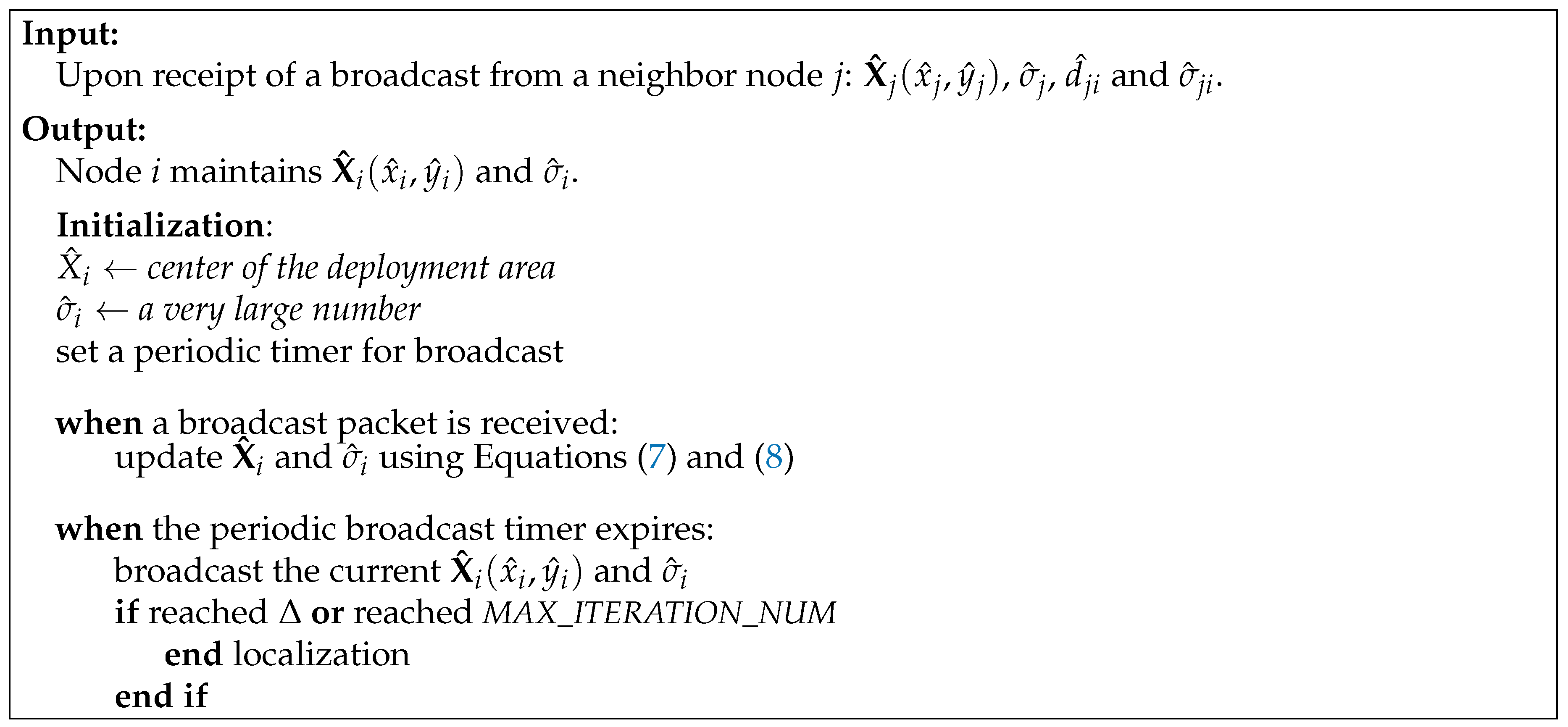
Figure 3 shows the algorithm that runs on each unknown node. The beacons only broadcast their positions.
3.3. KickLoc Kalman Algorithm
The KickLoc Intuitive algorithm (we call it KI in following sections) is very simple and parsimonious in terms of computation and memory storage. However, in the intuitive algorithm, the adjustment for the unknown node is made always on the line determined by the two nodes’ estimated position. This direction may not be the optimal adjustment (i.e., with regard to minimizing the variance of the position estimate) that can be obtained from the available measurement data (i.e., distance measurement ), and prior knowledge about node positions (i.e., position estimates of nodes and ). An extended Kalman filter can be used to determine the optimal update as we assume both the measurement model and the estimation states can be described using a Gaussian noise model.
In the KickLoc Kalman version (we call it KK in following sections.), each unknown node
i maintains its current position
with its error covariance
, and will update both once it receives a packet from its neighbor
j containing that neighbor’s current position
with its covariance
and the range estimate
with its variance
. The new position estimation is the current position adding an adjustment:
where,
If the estimated distance
is linear, then Equation (
1) becomes:
i.e., the minimization can be accomplished by applying the discrete Kalman filter. The resulting
and
are given by:
and
However, in our application, the estimated distance
is non-linear. Specifically in 2-D,
is:
Hence, Equation (
11) has to be linearized in order to apply the extended Kalman filter. The equation for the linearization of Equation (
11) at point
is:
where
is the Jacobian matrix of partial derivatives of
h with respect to
,
is the Jacobian matrix of partial derivatives of
h with respect to
,
and
is the Jacobian matrix of partial derivatives of
h with respect to
w,
After the linearization, the extended Kalman filter can then be applied to minimize the estimation error, which results in
,
, and
as:
In our application, for two-dimensional coordinates with the estimated distance given by Equation (
16), after solving the partial derivatives of
h with respect to
and
, it can be shown that
hence
Therefore Equation (
21) can be simplified:
The covariances
,
and
are known, the only unknown is
that can be easily obtained by plugging
in to the partial derivatives of
h with respect to
, which can be pre-calculated off-line once for all 2-D application.
Node
i will store its updated position
and its precision
by overwriting the previous one, and will repeat the update process when a new broadcast packet arrives. Using covariance matrix
and a square matrix with the number of rows and columns equal to
D, the dimensionality of the system, (i.e.,
for a 2D system and
for 3D.) The SD of node
i can be obtained as:
At the initial stage of the algorithm, the error covariance of an unknown node is set to infinity ( in 2-D), and in practice it is set to a large number (10,000 by default). The error covariance of a beacon node is set to 0 by default.
4. Simulation
In order to verify and test the performance of the proposed localization system, we build a simulation environment in MATLAB. We choose not to model the MAC, routing and transport layers, as typical networking issues in those layers (e.g., the routing algorithm, MAC fairness, etc.) should not influence the performance of the localization system, assuming that the updates are sufficiently infrequent to not cause congestion.
In
Section 4.1, the CRLB for multihop wireless sensor network localization is derived when the measurement distance error variance is not fixed. In
Section 4.2, both KickLoc Intuitive algorithm (KI) and KickLoc Kalman algorithm (KK) are tested in various networks to investigate the number of nodes that can be localized and the performance of the algorithms. In
Section 4.3, we first verify the convergence of the proposed algorthms, and then compare the
localization performance and
resource consumption performance of the Kick-based algorithms with other distributed, range-based localization systems, namely V-distance [
6], N-hop Multilateration [
9], and IWLSE [
10]. We also compare the localization precision with the theoretical CRLB derived in
Section 4.1.
Two localization performance metrics are used in the comparison: the accuracy of the localization, which calculates the difference between the ground-truth positions of the nodes and the estimated positions, and is determined using the mean of the differences; the precision of the localization, which calculates the uncertainty of the estimated positions, and is determined using the SD of the differences.
Three resource consumption performance metrics are used in the comparison, namely the memory consumption, computational consumption, and communication cost of the localization system.
All simulations are repeated 50 times unless otherwise specified to minimize the randomness introduced by the random deployment of nodes, and the randomly generated noise errors.
4.1. CRLB for Localization
The Cramér-Rao lower bound is a theoretical lower bound of the variance of an unbiased estimator [
28]. In this paper we use it as a benchmark for the performance evaluation of the localization estimator. This benchmark can be applied to any algorithm using range measurements to localize the unknowns.
The derivation of the CRLB of the variance in the estimated parameters is similar to the derivation in [
29]. In the derivation in [
29], the authors used a fixed variance
to represent the variance of each measurement distance error. In this paper, a diagonal matrix
is used to represent the variance of each measurement since we assume that the variance of a measurement depends on the distance [
10]. If the total number of measurements is
M,
will be an
matrix:
where
is the variance of the
measurement.
4.1.1. The Cramér-Rao Lower Bound
Suppose
is an unknown parameter vector to be estimated from observation vector
, which has a probability density function (PDF) of
. The lower bound of the variance of any unbiased estimator
of parameter
is defined as the inverse of the Fisher Information Matrix (FIM)
. By definition, the error covariance matrix of
is:
which is bounded by the CRLB as:
where the FIM
is defined as:
4.1.2. Deriving the CRLB for Multi-Hop Networks
In the context of multi-hop networks, the unknown parameter vector
to be estimated is a
vector:
where
A is the number of unknown nodes. The measurement vector
is a
vector of distance measurements
. We assume that each measurement
is white Gaussian, and the mean is the true distance
with standard deviation
.
The measurement probability density function (PDF) is the joint conditional PDF:
where
means node
i is a neighbor of node
j, hence a distance measurement can be obtained between the two. In matrix form:
Therefore the likelihood function is:
The CRLB can be calculated from Equation (
29):
From Equations (
1), (
30) and (
31):
where
is the
matrix with
element as
. If
corresponds to
, since
is either
or
for some corresponding node
,
The CRLB is then given by the inverse of the FIM as in Equation (
28). The CRLB for unknown node
i’s localization error becomes:
where
denotes the
element of the inverse matrix of
. The root-mean-squared error of the localization,
can be obtained by:
which represents the average variance lower bound for the localization error of the entire network.
4.2. KickLoc Verification and Analysis
For meaningful comparisons between different parameter settings, the estimation errors are normalized to the transmission range (i.e., a relative estimation error of 0.5 means half the transmission range). We define coverage as the ratio of unknown nodes that can be localized to the total number of unknown nodes. In DV-distance, N-hop Multilateration and IWLSE, a node can get a position estimation when it is connected to at least three beacons (one-hop or multi-hop). In KickLoc, unknown nodes keep updating its position estimation regardless of the number of beacons it is connected to. In this section, we define four criteria for nodes that can be localized to investigate the trade-off between coverage and localization error. The four criteria are based on the least number of beacons it requires for a node to be localized: zero connected beacons, one connected beacon, two connected beacons and three connected beacons. When evaluating the performance of localization under i connected beacons criterion, we only consider the performance of the unknown nodes that are connected to at least i beacons (single or multi-hop). Thus, for three connected beacon criterion, we only measure the performance of nodes that are connected to at least three beacons, while under the zero beacon criterion, all nodes are considered, even if completely isolated.
In simulating KickLoc algorithms, each node maintains a list of beacons that it is currently connected to (even multiple hops away), which is used to determine whether an unknown node is localized under different criteria (this beacon list is not maintained in the actual implementation, it is used here for performance analysis purpose). Coverage, relative estimation errors, and convergence process are investigated while considering different criteria for localization of an unknown node. In this subsection, a preset number of iterations (20 in simulation) and different criteria of being localized are used for better observation of convergence process; in all other sections a preset tolerance value () and three connected beacons criterion are used unless otherwise specified.
4.2.1. Dense Network
The first environment we test is a dense network with the following parameters:
Total number of nodes (beacons and unknowns): 200
Area: 100 m × 100 m
Transmission range: 30 m
Beacon to total nodes ratio: 0.2
Standard deviation of the distance measurement d, : (20% of the distance measurement.)
Figure 4 shows an example network topology generated in MATLAB. The simulation with same parameters (but different randomly generated topologies) is then repeated 100 times, and the resulting average connectivity (i.e., the average number of neighbors for each node) of the network is 41.66. In such a dense network, all unknown nodes are connected to 3 or more beacons (albeit through multi-hop), therefore the coverage is 100% for both algorithms and all beacon number criteria.
Figure 5a shows the cumulative distribution function (CDF) of relative localization errors for the two algorithms. KI achieves a confidence interval with confidence level 90% for the relative error of (−0.22, +0.22), and the 50% accuracy is less than 0.11; KK achieves a confidence interval of (−0.48, +0.48), and the 50% accuracy is less than 0.1.
Figure 5b verifies the convergence of KI and KK, as each algorithm has an initial steep drop and converges after only a few iterations.
4.2.2. Sparse Network
The performance of the algorithms are also investigated in a relatively sparse network with the number of nodes reduced from 200 to 30, and the transmission range reduced from 30 m to 20 m.
An example network topology is shown in
Figure 6. The simulation is again repeated 100 times, and the resulting average connectivity is 3.07. Under
zero connected beacon criterion, KI and KK both achieve a confidence interval with confidence level 90% for the relative error of (−2.50, +2.50), and achieve the 50% accuracy of 0.75. Under
one connected beacon or more criterion, KI and KK both achieve a confidence interval with confidence level 90% for the relative error of about (−1.89, +1.89), and achieve the 50% accuracy of 1.06. The coverage with
one connected beacon criterion is 79.42%, with
two connected beacons criterion is 59.13%, and
three connected beacons criterion is 47.00%.
Figure 7 verifies the convergence of KI and KK with different beacon criteria. Again each algorithm converges after a limited number of iterations regardless of the beacon criteria.
The results from both sparse and dense networks verifies the convergence of both KI and KK. The localization errors in sparse networks are much higher than in dense networks, which is expected as sparse networks have much lower average connectivity, and therefore unknown nodes are more likely to be disconnected or far from any beacons, or in a corner. KK is supposed to perform better than KI as KI has more relaxed assumptions (i.e., the adjustment is on the line determined by the two nodes’ position estimation), but actually KK shows very similar results to KI. This is due to the fact that KK’s performance is affected by the errors generated in the linearization process of function : the measurement function h is non-linear and cannot be accurately estimated by the linearization. In addition, this transformation error cannot be estimated and therefore it is not reflected in the estimation error covariance . Therefore, when a relatively high localization error occurs on one unknown, it will negatively influence other nodes because this particular node falsely claims a high precision.
4.3. Performance Evaluation and Comparison
With the aforementioned simulator in MATLAB, a series sets of tests have been performed to obtain measurements on different performance metrics of the system. We vary network parameters including the number of nodes, area size, transmission range, beacon to total nodes ratio and distance measurement error standard deviation to evaluate the localization performance.
Table 1 lists a set of standard parameter values that we choose, from which one value is changed at a time to test the systems sensitivity to that particular parameter.
Under the standard scenario, the average connectivity of the network is 10.4224, the mean and SD of the relative estimation error are (0.4557, 0.4613) for KI, (0.4777, 0.4648) for KK, (0.6179, 0.3674) for DV-distance, (0.5094, 0.4053) for N-hop Multilateration, (0.5015, 0.4513) for IWLSE. The SD of the relative estimation error for CRLB is 0.2337. The coverages of the five algorithms are 100%.
4.3.1. Convergence Verification
In DV-distance, N-hop Multilateration and IWLSE, after the “DV-distance propagation” (though different approach to get the multi-hop distance), unknown nodes with distance estimates of more than two beacons can perform multi-lateration (for DV-distance and IWLSE) or bounding box (for N-hop Multilateration) to obtain their localization estimates. In N-hop Multilateration and IWLSE, these localization estimates serve as an initial estimate, and an iterative refinement phase follows to improve the localization performance. In KickLoc algorithms, there’s no need to establish the “DV-distance propagation” first, as the iterative refinement phase starts at the very beginning of the process. Since the localization procedure is different for each algorithm, the iteration steps cannot be directly compared for the different algorithms. To illustrate the convergence trends at different network densities,
Figure 8a shows the average number of iterations for each algorithm as a function of the number of nodes in the network. All the algorithms converge within five iterations unless it is a very sparse network. When the network is very sparse, most of the unknown nodes cannot reach the preset tolerance value (
in simulation), hence will keep iterating until reaching the maximum preset iteration steps (20 in simulation).
4.3.2. Localization Accuracy and Precision
For localization performance comparison, a series of simulations are conducted with varying network parameters summarized in
Table 1, namely the number of nodes, beacon to total nodes ratio and distance measurement error SD.
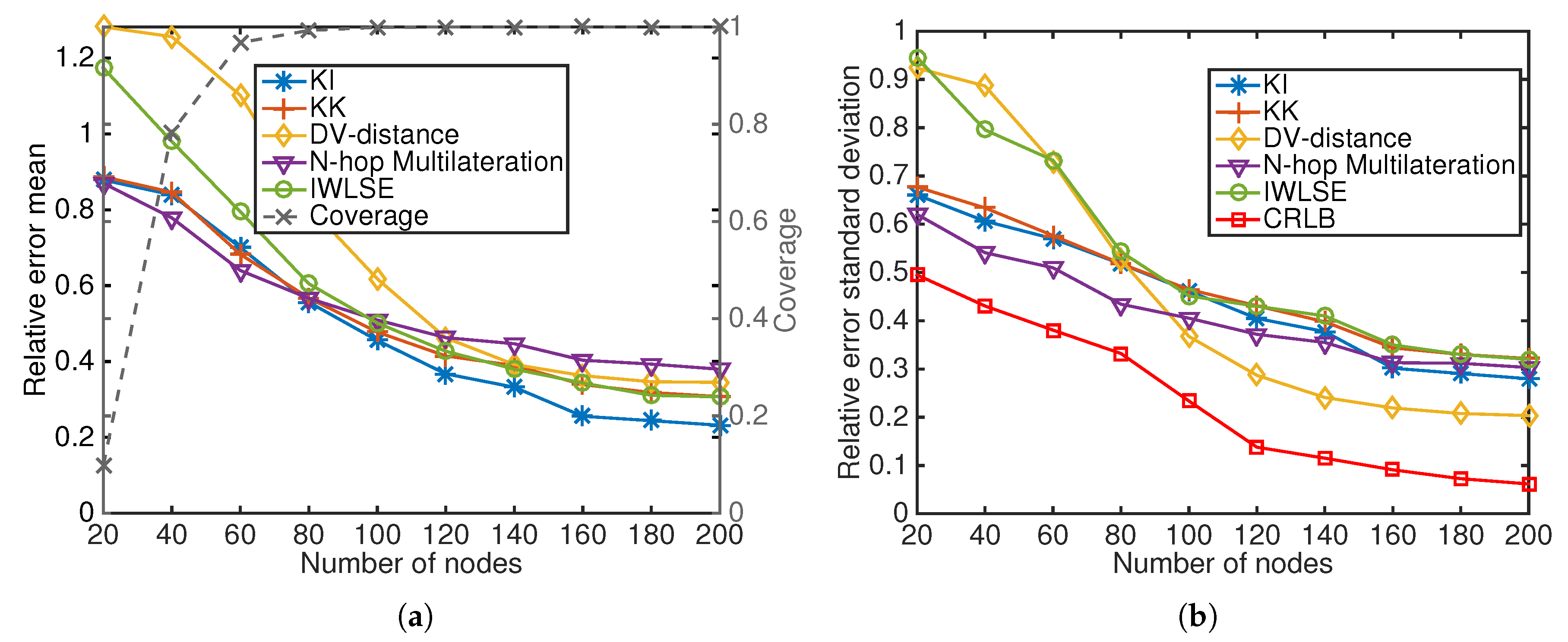
Number of nodes:Figure 9 indicates that the relative error mean and SD decrease when the number of nodes increases for all algorithms. Increasing the number of nodes leads to higher average connectivity when other parameters remain the same, which increases the information available for localization. DV-distance and IWLSE do not perform well when the number of nodes is small, because DV-based distance correction works poorly in sparse anisotropic networks. N-hop Multilateration does not perform well at high number of nodes, because in its refinement stage, it leverages estimates from all its neighbors without estimation precision information. KickLoc algorithms have good performance at both low and high number of nodes.
Area size: when the area size of the network increases, the relative error mean and SD increase for all algorithms as shown in
Figure 10. The result is consistent with results of changing number of nodes, as they are both changing the density of the network when other parameters are kept the same.
Transmission range: if we increase the transmission range of the transceivers, the number of neighbors in the network is increasing, but the distance measurement error also increases, which results in a trade-off between the benefit from more distance information and the shortcomings of highly noisy distance information.
Figure 11 illustrates that both the DV-based distance correction used in DV-distance and IWLSE, and leveraging the precision of measurements in KickLoc algorithms and IWLSE can effectively mitigate the highly noisy distance information. When the transmission range is very large, N-hop Multilateration works poorly as it does not have a strategy to alleviate the noisy distance measurement. Note that KK also works poorly with the high measurement error, which is due to the large linearization error in this scenario.
Beacon to total nodes ratio: in this scenario we change the beacon ratio from 0.03 (resulting in 3 beacon nodes which is the minimum requirement for 2-D multilateration.) to 0.3.
Figure 12 shows that DV-Distance has a slightly different performance trend from all other algorithms. DV-Distance only updates position estimations from beacon nodes, therefore it is immune to the large errors from neighbors when the beacon ratio is small, but it does not benefit from the updates from neighbors when beacon ratio is large. Kick-based algorithms perform better than the other algorithms when the beacon ratio becomes very high.
Measurement error standard deviation: As expected, each algorithm has an increasing relative error with an increasing measurement error SD (
Figure 13). DV-Distance and N-hop Multilateration work poorly when the measurement error SD becomes large, mainly because they do not take the reliability of measurements into account during the process. KickLoc algorithms have much better performance in both error mean and SD when the measurement error is very high.
4.3.3. Memory Consumption
Wireless sensors are usually constraint by their physical size and unit cost, which in return limits their memory space for data and code storage. Many commercial sensor platforms have RAM size smaller than 10 KB, and flash storage less than 1 MB [
30]. For instance, the widely-used sensor platform MICA2 only has 4 KB RAM and 128 KB flash storage; another popular sensor type TelosB has 10 KB RAM and 1024 KB flash storage. Therefore, the data storage for the localization process must be able to fit it in the limited memory space of a sensor node. We analyze how much working storage each method needs (i.e., the maximum amount of memory needed at any point of the process on the node).
Let denote the amount of working storage an algorithm needs; denotes all the unknown nodes in the network, denotes the number of beacons node i is connected to, albeit multi-hop, denotes the number of neighbors of node i, and denotes the neighbor list of node i.
In DV-distance, node
i has to store its own position estimate (
) (2 bytes), its own “DV-distance propagation” (
bytes), an incoming “DV-distance propagation” from neighbor j (
bytes), a distance estimate between node
i and
j obtained from the extracted RSSI (1 byte), a
matrix
and a
matrix
for the multilateration between beacon nodes (
). Therefore DV-distance requires:
bytes of space. Hence the space complexity of DV-distance is
which is determined by
for
.
In N-hop Multilateration, node
i has to store its own position estimate (
) (2 bytes), its own “DV-distance propagation” (
bytes), an incoming “DV-distance propagation” from neighbor j (
bytes), a distance estimate between node
i and
j obtained from the extracted RSSI (1 byte), a bounding box for the initial estimation phase (4 bytes), a
matrix
and a
matrix
for the multilateration between neighbors in the refinement phase. Therefore N-hop Multilateration requires:
bytes of space. Hence the space complexity of the algorithm is
which is collectively determined by
and
for
.
In IWLSE, node
i has to store its own position estimate (
) and estimation standard deviation (3 bytes), its own “DV-distance propagation” (
since it added an estimation standard deviation of the “DV-distance propagation”), an incoming “DV-distance propagation” from neighbor j (
), a distance estimate along with a standard deviation between node
i and
j obtained from the extracted RSSI (2 bytes), a
matrix
and a
matrix
between beacons in the initial estimation phase and a
matrix
and a
matrix
between beacons in the refinement phase. Therefore IWLSE requires:
bytes of space. Hence the space complexity is the same as N-hop Multilateration.
In KickLoc algorithms, since the algorithm does not need to conduct the “DV-distance propagation”, and the localization phase does not rely on multi-lateration or bounding box, the memory storage is not dependent on or . The bytes required for KI and KK are 12 bytes and 21 bytes respectively, therefore a space complexity of .
4.3.4. Computational Consumption
To analyze how much computation has been consumed for each sensor node to get localized is sometimes important as it adds extra burden to the limited battery life and computing resources available on the sensor node. The computational cost can be evaluated using the Lightspeed toolbox available in MATLAB [
31] which counts the number of floating-point operations (FLOPs) performed. This FLOP counting tool allows comparisons of numerical algorithms independent of programming language and machine used, as it manually outputs the minimal number of FLOPs the algorithm needs. Moreover, this manual flop counting feature allows us to focus on the computational cost generated by the localization algorithm itself, in isolation from unrelated operations.
To examine how number of FLOPs changes when the network density varies, we change the number of nodes from 20 to 200, and the resulting total number of FLOPs consumed for each algorithm is shown in
Figure 8b. For 20 nodes, the KickLoc algorithms consume more FLOPs than other algorithms. From the convergence result in
Section 4.3.1, we know that when the network is very sparse, most of the unknown nodes cannot reach the preset tolerance value, hence will keep iterate until reaching the maximum preset iteration steps. Some of the unknown nodes cannot even be localized at all since they do not have connection to more than two beacons, albeit multi-hop. In DV-distance, N-hop Multilateration and IWLSE, unknown nodes in this case will not initiate the lateration computation since they do not have enough beacon nodes. In KickLoc algorithms, this can be achieved if each node maintains a list of beacons that it is currently connected to as we mentioned in
Section 4.2. To preserve the simplicity of the algorithms, we do not use this feature by default, but it can be enabled if KickLoc is used in very sparse network. For networks larger than 40 nodes, KickLoc algorithms start to use fewer FLOPs, and show much better scalability than the other algorithms.
4.3.5. Communication Cost
As energy constraint is of great importance in WSNs, and network communication is a major consumer of the energy consumption, it is very important to minimize the communication cost of the application.
Figure 8c,d show the communication cost both at the packet level and at the byte level at different network densities. When the number of nodes is 20, all algorithms except DV-distance have to go through a long iteration process, as they cannot reach the preset tolerance value. For networks larger than 40 nodes, all algorithms have increasing communication cost as the number of nodes increases. The cause of the large difference between the KickLoc and other algorithms is two-fold. First, KickLoc does not need to conduct the “DV-distance propagation”, which consumes a large amount of message exchanges. Second, the packet size of both KickLoc algorithms are fixed and very small (18 bytes for KI and 21 bytes for KK). The difference between DV-distance, N-hop Multilateration and IWLSE is due to different average iteration steps of N-hop Multilateration and IWLSE as shown in
Figure 8a, and no iteration process for DV-distance. The information exchange method at the packet level is exactly the same for both KickLoc algorithms, the minor difference in
Figure 8c is due to the slightly different average iteration steps; at the byte level, KI has the smallest communication cost as it has the smallest packet size.
5. Experiments
In this section, the localization performance of the proposed algorithms are evaluated using both RSSI and acoustic measurements. Before the performance evaluation, we have made improvements to the original KickLoc to further reduce the localization error.
5.1. Improvements to KickLoc
In
Section 4, it is verified that KickLoc algorithms can achieve reasonable localization with very low resource consumption. However, after further examining the process of the algorithms, we realise that the localization results can be further improved by modifications to our original algorithms.
5.1.1. Correction of the Initial Update
In the original KI and KK, we set the initial position estimate of each unknown node at the center of the deployment space, therefore we are able to handle the initial Kick update just the same as all the subsequent updates, which is in fact not optimal. For example, in
Figure 14, unknown node
i will set its initial estimation at the center of deployment, marked as a black cross. After receiving a broadcast message from node
j, a normal Kick calculation is performed and will result in an updated position estimation, which can be represented by a grid circle in the illustration. However, in reality, when no prior information is available on node
i, after node
j’s message, the position estimation of node
i should be a ring-shaped region determined by node
j’s position uncertainty, the distance measurement
d and its noise.
5.1.2. Introduction of Linearization Noise to KK
In
Section 4, KK does not always exhibit a better localization result than KI, though it supposes to provide a more accurate kick. The performance of the EKF system is greatly dependent on the modelling accuracy of noise in the system. In our application, after the linearzation in Equation (
17), all the higher order terms of the observation noise are ignored. The observation noise can be more precisely modelled if this new “linearization noise” is taken into account. The residual
can be rewritten as:
where
w represents the distance measurement noise, and
o represents the linearization noise. It is shown in [
32] that the linearization noise can be precisely approximated using an adaptive Kalman filter. To be consistent with the simple design paradigm of this system, a fixed linearization noise that can achieve comparable result is used.
In the remainder of this section, the performance of the improved KickLoc algorithms (we call them KI-imp and KK-imp respectively) will be evaluated along with other algorithms.
5.2. RSSI Experiment Evaluation
We use the widely-used TI CC2530 system-on-chip (SoC) [
33] to verify the measurement model we used in the simulation, and also to test the feasibility of implementing our proposed system in a realistic, resource-limited, sensor platform. Unfortunately, we have only conducted experiments with small scaled topology, as we have limited number of CC2530 units available. However, it should be sufficient to serve our purpose as we have shown in the simulation that the system is fully scalable, and the memory consumption is independent of the network size.
5.2.1. Overview of CC2530 and Contiki OS
The CC2530 SoC is a Texas Instruments solution for 2.4 GHz ZigBee applications. It is designed to form robust sensor networks with ultra low total unit costs. It has an industry-standard enhanced 8051 MCU, 8-KB RAM, and 256 in-system programmable flash storage. Contiki [
34] is a C based, open source operating system for sensor networks, which is lightweight, portable, yet powerful.
5.2.2. Experiment Setup
We conduct the experiment on an outdoor grass field. Fifteen CC2530 sensor nodes are randomly deployed within a 10 m × 10 m rectangular area. Five of them are configured as beacon nodes, and the rest are configured as unknown nodes. We also program each node to periodically broadcasts its position estimate and the estimated uncertainty, and locally updates its estimate upon receiving an update. The process continues until all nodes transmit 100 packets. Although our system is fully distributed and only keeps the current state, all the logs are stored during the experiment to better analyze the refining process later off-line. The experiment took place when no people were near the area.
5.2.3. RSSI Calibration and Measurement Model Fitting
It is well-received that low power ZigBee radios exhibits notoriously high RSSI variability [
35,
36]. Our calibration results (
Figure 15a) also shows high RSSI variability. We fit the RSSI vs. distance mapping data from our calibration process to the RSSI measurement model we used in our simulation [
37], which results in a path loss exponent n equals to 2.36, and the SD of distance measurement error to be
. The fitting result is shown in
Figure 15b. Both the raw data direct mapping and the fitted model are later used in the localization experiment.
5.2.4. RSSI Experimental Results
Figure 16 demonstrates the position estimate and the estimated uncertainty on each unknown node at the end of the experiment for one random generated topology described in
Section 5.2.2 when using KK algorithm. The same experiment was conducted multiple times, and the proposed algorithms are shown to be effective in that the position estimate of an unknown always fall in the estimated bounds as long as the unknown can be localized.
Figure 17 summarizes the resulting mean localization errors for all the localization algorithms under the two measurement models. Interestingly, the results show that the fitting model that we used in the simulation actually improves the localization accuracy for all the algorithms tested. KickLoc again achieves higher localization accuracy despite the high RSSI variability on the ZigBee radios.
Figure 16 shows the final estimation results of one run using KK. The real position of the unknowns are shown as the red dots, and the position estimates are marked by the black crosses. The estimated uncertainty of an unknown is shown by an ellipse (circles when using KI), and the semi-axes of the ellipse are
of the estimated uncertainty distribution (modeled as Gaussian), in
x and
y directions.
5.3. Acoustic Experiment Evaluation
Simulation and experimental results with RSSI have verified that KickLoc is suitable for WSNs with distance measurement noise that are relatively large and proportional to distance. The system is designed to work with various distance measurement models, therefore we also test it with an acoustic platform, which utilizes TOA (time of arrival) measurements that have relatively small noise and the noise is not dependent of the distance [
38].
5.3.1. Biobotic Sensor Network Platform
In [
39], we designed a biobotic sensor network platform for acoustic localization. In the project, insect biobots equipped with neurostimulation backpacks are the sensor nodes in the network. RF signals and acoustic signals are combined to obtain a more fine-grained range measurement and therefore achieve high-accuracy, real-time localization of the biobotic nodes.
A specially designed miniature backpack (
Figure 18) is carried by a cockroach. All the components used to make the backpack are commercially available off-the-shelf. Each biobot is programmed to periodically buzz and radio broadcast at the same time. As the speed of RF propagation is much faster than the speed of sound, the range information between the cockroach agents can be approximated as the multiplication of the TOA (time difference between the receipt of the concurrently emitted RF and acoustic signal) and the speed of sound. Digital processing and peak detection methods are used to efficiently determine the TOA from the raw readings. Details about the backpack, and the system design can be referred to in [
39].
5.3.2. Additive Noise Compensation
After obtaining the TOA, the distance between the biobotic sensor nodes can be calculated by multiplying the speed of sound. An additive constant time noise introduced by internal processing delays [
38,
40] has to be compensated for a more accurate TOA estimation.
We conducted the calibrations by placing the transceivers in a room with no obstacles in between, and the distance between the two was varied from 1 to 5 m. The data collection was repeated 10 times at each spot. The collected data are then applied to a linear regression to tune the additive internal delay.
Figure 19a shows the real distances and the calculated distances, which verifies the existence of the additive delay. The linear regression results in a fitted additive delay of 0.68 ms.
Figure 19b shows that after the compensation, the ranging errors decrease significantly (the mean ranging error reduces by about 20 cm).
5.3.3. Acoustic Experimental Results
Owing to the very limited number of biobotic sensor agents available, a proof-of-concept implementation with six sensor nodes is performed. Four beacons and two unknown nodes are randomly deployed in a 5 m × 5 m indoor environment. In this sparse network, other algorithms (DV-distance, N-hop Multilateration, and IWLSE) cannot perform properly. Therefore we only compare the results of KI, KK, KI-imp and KK-imp.
Figure 20 demonstrates the position estimate and the estimated uncertainty on each unknown node at the end of the experiment for one random generated topology when using KK-imp algorithm. The average localization errors of multiple runs are shown in
Figure 21. The Kalman filter based algorithms perform better than the intuitive algorithms, and the improved version of the original algorithms also reduces the localization error.
6. Conclusions
In this paper, we presented a lightweight localization solution for small, low resources WSNs, which bridges the gap between high accuracy performance demand in localization and low resources available in sensor networks. The solution is fully distributed, and achieves high localization performance by considering the uncertainty of the distance measurements to minimize localization errors introduced from the range measurement, and fuses information from all neighboring nodes. Extensive simulations validated the feasibility, performance and robustness of the system. We also implemented both the intuitive and the Kalman filter based algorithms on TI CC2530 ZigBee SoC and our customized acoustic platforms. The results show that KickLoc is able to provide consistent location estimation under different measurement models. In the future, we would like to extend the system from 2-D to 3-D, and test the system in mobile sensor networks.
Author Contributions
Conceptualization, H.X. and M.L.S.; Investigation, H.X.; Methodology, H.X. and M.L.S.; Software, H.X.; Supervision, M.L.S.; Validation, H.X.; Writing—original draft, H.X.; Writing—review and editing, H.X. and M.L.S.
Funding
This work was supported in part by the National Science Foundation under the Cyber-physical Systems Program (CNS-1239243).
Acknowledgments
The authros would like to thank Tahmid Latif and Talha Agcayazi for their assistance with the experimental hardware.
Conflicts of Interest
The authors declare no conflict of interest.
Abbreviations
The following abbreviations are used in this manuscript:
| WSN | Wireless sensor network |
| CRLB | Cramér-Rao lower bound |
| RSSI | Received signal strength indicator |
| TOA | Time of arrival |
| IWLSE | Iterative weight least squares estimation |
| AUV | autonomous underwater vehicle |
| LSQ | Least squares solver |
| EKF | Extended Kalman filter |
| RF | Radio frequency |
| SD | Standard deviation |
| FIM | Fisher Information Matrix |
| PDF | Probability density function |
| CDF | Cumulative distribution function |
| FLOPs | Floating-point operations |
| SoC | System-on-chip |
References
- Yue, Y.G.; He, P. A comprehensive survey on the reliability of mobile wireless sensor networks: Taxonomy, challenges, and future directions. Inf. Fusion 2018, 44, 188–204. [Google Scholar] [CrossRef]
- Tan, X.; Sun, Z.; Akyildiz, I.F. Wireless Underground Sensor Networks: MI-based communication systems for underground applications. IEEE Antennas Propag. Mag. 2015, 57, 74–87. [Google Scholar] [CrossRef]
- Malaver, A.; Motta, N.; Corke, P.; Gonzalez, F. Development and integration of a solar powered unmanned aerial vehicle and a wireless sensor network to monitor greenhouse gases. Sensors 2015, 15, 4072–4096. [Google Scholar] [CrossRef] [PubMed]
- Rabaey, C.S.J.; Langendoen, K. Robust positioning algorithms for distributed ad-hoc wireless sensor networks. In Proceedings of the General Track of the Annual Conference on USENIX Annual Technical Conference, Monterey, CA, USA, 10–15 June 2002; pp. 317–327. [Google Scholar]
- Chiang, C.T.; Tseng, P.H.; Feng, K.T. Hybrid unified Kalman tracking algorithms for heterogeneous wireless location systems. IEEE Trans. Veh. Technol. 2012, 61, 702–715. [Google Scholar] [CrossRef]
- Niculescu, D.; Nath, B. DV based positioning in ad hoc networks. Telecommun. Syst. 2003, 22, 267–280. [Google Scholar] [CrossRef]
- Wang, J.; Ghosh, R.K.; Das, S.K. A survey on sensor localization. J. Control Theory Appl. 2010, 8, 2–11. [Google Scholar] [CrossRef] [Green Version]
- Amundson, I.; Koutsoukos, X.D. A survey on localization for mobile wireless sensor networks. In Mobile Entity Localization and Tracking in GPS-Less Environnments; Springer: Berlin/Heidelberg, Germany, 2009; pp. 235–254. [Google Scholar]
- Savvides, A.; Park, H.; Srivastava, M.B. The bits and flops of the n-hop multilateration primitive for node localization problems. In Proceedings of the 1st ACM International Workshop on Wireless Sensor Networks and Applications, Atlanta, GA, USA, 28 September 2002; ACM: New York, NY, USA, 2002; pp. 112–121. [Google Scholar]
- Evers, L.; Dulman, S.; Havinga, P. A distributed precision based localization algorithm for ad-hoc networks. In Pervasive Computing; Springer: Berlin/Heidelberg, Germany, 2004; pp. 269–286. [Google Scholar]
- Garcia, M.; Tomas, J.; Boronat, F.; Lloret, J. The Development of Two Systems for Indoor Wireless Sensors Self-location. Ad Hoc Sens. Wirel. Netw. 2009, 8, 235–258. [Google Scholar]
- Garcia, M.; Martinez, C.; Tomas, J.; Lloret, J. Wireless sensors self-location in an indoor WLAN environment. In Proceedings of the 2007 International Conference on Sensor Technologies and Applications (SENSORCOMM 2007), Valencia, Spain, 14–20 October 2007; IEEE: Piscataway, NJ, USA, 2007; pp. 146–151. [Google Scholar]
- Parkinson, B.W.; Spilker, J.J. Progress in Astronautics and Aeronautics: Global Positioning System: Theory and Applications; AIAA: Reston, VA, USA, 1996. [Google Scholar]
- Langendoen, K.; Reijers, N. Distributed localization in wireless sensor networks: A quantitative comparison. Comput. Netw. 2003, 43, 499–518. [Google Scholar] [CrossRef]
- Kalman, R.E. A New Approach to Linear Filtering and Prediction Problems. Trans. ASME Basic Eng. 1960, 82, 35–45. [Google Scholar] [CrossRef] [Green Version]
- Olson, E.; Leonard, J.J.; Teller, S. Robust range-only beacon localization. IEEE J. Ocean. Eng. 2006, 31, 949–958. [Google Scholar] [CrossRef]
- Sreenath, K.; Lewis, F.L.; Popa, D.O. Simultaneous adaptive localization of a wireless sensor network. ACM SIGMOBILE Mob. Comput. Commun. Rev. 2007, 11, 14–28. [Google Scholar] [CrossRef]
- Pathirana, P.N.; Bulusu, N.; Savkin, A.V.; Jha, S. Node localization using mobile robots in delay-tolerant sensor networks. IEEE Trans. Mob. Comput. 2005, 4, 285–296. [Google Scholar] [CrossRef] [Green Version]
- Rocco, M.D.; Pascucci, F. Sensor network localisation using distributed extended kalman filter. In Proceedings of the 2007 IEEE/ASME International Conference on Advanced Intelligent Mechatronics, Zurich, Switzerland, 4–7 September 2007; IEEE: Piscataway, NJ, USA, 2007; pp. 1–6. [Google Scholar]
- Xiong, H.; Sichitiu, M.L. KickLoc: Simple, Distributed Localization for Wireless Sensor Networks. In Proceedings of the 2016 IEEE 13th International Conference on Mobile Ad Hoc and Sensor Systems (MASS), Brasilia, Brazil, 10–13 October 2016; IEEE: Piscataway, NJ, USA, 2016; pp. 228–236. [Google Scholar]
- Smith, A.; Balakrishnan, H.; Goraczko, M.; Priyantha, N. Tracking moving devices with the cricket location system. In Proceedings of the 2nd International Conference on Mobile Systems, Applications, and Services, Boston, MA, USA, 6–9 June 2004; ACM: New York, NY, USA, 2004; pp. 190–202. [Google Scholar]
- Caceres, M.A.; Sottile, F.; Spirito, M.A. Adaptive location tracking by kalman filter in wireless sensor networks. In Proceedings of the IEEE International Conference on Wireless and Mobile Computing, Networking and Communications (WIMOB), Marrakech, Morocco, 12–14 October 2009; IEEE: Piscataway, NJ, USA, 2009; pp. 123–128. [Google Scholar]
- Tseng, P.H.; Feng, K.T.; Lin, Y.C.; Chen, C.L. Wireless location tracking algorithms for environments with insufficient signal sources. IEEE Trans. Mob. Comput. 2009, 8, 1676–1689. [Google Scholar] [CrossRef]
- Dissanayake, M.G.; Newman, P.; Clark, S.; Durrant-Whyte, H.F.; Csorba, M. A solution to the simultaneous localization and map building (SLAM) problem. IEEE Trans. Robot. Autom. 2001, 17, 229–241. [Google Scholar] [CrossRef] [Green Version]
- Fenwick, J.W.; Newman, P.M.; Leonard, J.J. Cooperative concurrent mapping and localization. In Proceedings of the IEEE International Conference on Robotics and Automation, ICRA’02, Washington, DC, USA, 11–15 May 2002; IEEE: Piscataway, NJ, USA, 2002; Volume 2, pp. 1810–1817. [Google Scholar]
- Maybeck, P.S. Stochastic Models, Estimation, and Control; Academic Press: New York, NY, USA, 1982; Volume 3. [Google Scholar]
- Whitehouse, K.; Culler, D. Calibration as parameter estimation in sensor networks. In Proceedings of the 1st ACM International Workshop on Wireless Sensor Networks and Applications, Atlanta, GA, USA, 28 September 2002; ACM: New York, NY, USA, 2002; pp. 59–67. [Google Scholar]
- Kay, S.M. Fundamentals of Statistical Signal Processing: Estimation Theory; Prentice-Hall: Englewood Cliffs, NJ, USA, 2010; Volume 1. [Google Scholar]
- Savvides, A.; Garber, W.; Adlakha, S.; Moses, R.; Srivastava, M.B. On the error characteristics of multihop node localization in ad-hoc sensor networks. In Information Processing in Sensor Networks; Springer: Berlin/Heidelberg, Germany, 2003; pp. 317–332. [Google Scholar]
- Healy, M.; Newe, T.; Lewis, E. Wireless sensor node hardware: A review. In Proceedings of the 2008 IEEE Sensors, Lecce, Italy, 26–29 October 2008; IEEE: Piscataway, NJ, USA, 2008; pp. 621–624. [Google Scholar]
- Minka, T. The Lightspeed Matlab Toolbox. Available online: http:// research.microsoft.com/en-us/um/people/minka/software/lightspeed/ (accessed on 14 January 2016).
- Xiong, H. Simple, Distributed Localization and Tracking for Wireless Sensor Networks. Ph.D. Dissertation, North Carolina State University, Raleigh, NC, USA, 2019. [Google Scholar]
- Texas Instruments: CC253x/4x User’s Guide (Rev. F). 2014. Available online: http://www.ti.com/lit/ug/swru191f/swru191f.pdf (accessed on 29 April 2019).
- Dunkels, A.; Grönvall, B.; Voigt, T. Contiki-a lightweight and flexible operating system for tiny networked sensors. In Proceedings of the 29th Annual IEEE International Conference on Local Computer Networks, Tampa, FL, USA, 16–18 November 2004; IEEE: Piscataway, NJ, USA, 2004; pp. 455–462. [Google Scholar]
- Lymberopoulos, D.; Lindsey, Q.; Savvides, A. An empirical characterization of radio signal strength variability in 3-D IEEE 802.15. 4 networks using monopole antennas. In Wireless Sensor Networks; Springer: Berlin/Heidelberg, Germany, 2006; pp. 326–341. [Google Scholar]
- Xiong, H.; Latif, T.; Lobaton, E.; Bozkurt, A.; Sichitiu, M. Characterization of RSS Variability for Biobot Localization Using 802.15.4 Radios. In Proceedings of the IEEE Topical Conference on Wireless Sensors and Sensor Networks (WiSNet), Austin, TX, USA, 24–27 January 2016. [Google Scholar]
- Rappaport, T.S. Wireless Communications: Principles and Practice, 1st ed.; IEEE Press: Piscataway, NJ, USA, 1996. [Google Scholar]
- Patwari, N.; Ash, J.N.; Kyperountas, S.; Hero, A.O.; Moses, R.L.; Correal, N.S. Locating the nodes: Cooperative localization in wireless sensor networks. IEEE Signal Process. Mag. 2005, 22, 54–69. [Google Scholar] [CrossRef]
- Xiong, H.; Agcayazi, T.; Latif, T.; Bozkurt, A.; Sichitiu, M.L. Towards acoustic localization for biobotic sensor networks. In Proceedings of the 2017 IEEE SENSORS, Glasgow, UK, 29 October–1 November 2017; IEEE: Piscataway, NJ, USA, 2017; pp. 1–3. [Google Scholar]
- Sallai, J.; Balogh, G.; Maroti, M.; Ledeczi, A.; Kusy, B. Acoustic Ranging in Resource-Constrained Sensor Networks. In Proceedings of the International Conference on Wireless Networks, Las Vegas, NV, USA, 21–24 June 2004; p. 467. [Google Scholar]
Figure 1.
An example network topology consists of three beacons and three unknown nodes . An edge is drawn between each pair of nodes that can directly communicate with each other.
Figure 1.
An example network topology consists of three beacons and three unknown nodes . An edge is drawn between each pair of nodes that can directly communicate with each other.
Figure 2.
Illustrations of the intuition of the position adjustment in two scenarios: (a) when measured distance is smaller than expected distance, kick it closer; (b) when measured distance is larger than expected distance, kick it further.
Figure 2.
Illustrations of the intuition of the position adjustment in two scenarios: (a) when measured distance is smaller than expected distance, kick it closer; (b) when measured distance is larger than expected distance, kick it further.
Figure 3.
KickLoc Intuitive algorithm that runs on unknown node i.
Figure 3.
KickLoc Intuitive algorithm that runs on unknown node i.
Figure 4.
An example network topology generated in MATLAB with 40 beacons and 160 unknowns in a 100 m × 100 m area.
Figure 4.
An example network topology generated in MATLAB with 40 beacons and 160 unknowns in a 100 m × 100 m area.
Figure 5.
(a) CDF of relative localization error for KI and KK in dense networks. (b) Relative localization error as a function of the number of iterations for KI and KK in dense networks.
Figure 5.
(a) CDF of relative localization error for KI and KK in dense networks. (b) Relative localization error as a function of the number of iterations for KI and KK in dense networks.
Figure 6.
An example sparse network topology consists of six beacons and 24 unknown nodes.
Figure 6.
An example sparse network topology consists of six beacons and 24 unknown nodes.
Figure 7.
Relative localization error and coverage in sparse networks as a function of number of iterations for KI and KK with (a) zero connected beacon criterion, (b) one connected beacon criterion, (c) two connected beacons criterion, and (d) three connected beacons criterion.
Figure 7.
Relative localization error and coverage in sparse networks as a function of number of iterations for KI and KK with (a) zero connected beacon criterion, (b) one connected beacon criterion, (c) two connected beacons criterion, and (d) three connected beacons criterion.
Figure 8.
Performance results as a result of changing the number of nodes: (a) average number of iterations, (b) total number of FLOPs consumed, (c) total messages sent, and (d) total bytes sent.
Figure 8.
Performance results as a result of changing the number of nodes: (a) average number of iterations, (b) total number of FLOPs consumed, (c) total messages sent, and (d) total bytes sent.
Figure 9.
(a) Average estimation error and coverage, (b) SD as a result of changing the number of nodes.
Figure 9.
(a) Average estimation error and coverage, (b) SD as a result of changing the number of nodes.
Figure 10.
(a) Average estimation error and coverage, (b) SD as a result of changing the area size.
Figure 10.
(a) Average estimation error and coverage, (b) SD as a result of changing the area size.
Figure 11.
(a) Average estimation error and coverage, (b) SD as a result of changing the transmission range.
Figure 11.
(a) Average estimation error and coverage, (b) SD as a result of changing the transmission range.
Figure 12.
(a) Average estimation error and coverage, (b) SD as a result of changing the beacon to total nodes ratio.
Figure 12.
(a) Average estimation error and coverage, (b) SD as a result of changing the beacon to total nodes ratio.
Figure 13.
(a) Average estimation error and coverage, (b) SD w.r.t. different measurement error SDs.
Figure 13.
(a) Average estimation error and coverage, (b) SD w.r.t. different measurement error SDs.
Figure 14.
Example scenario when unknown node i gets initial broadcast message from neighbor node j, with a distance measurement of d. The black cross is the center of the whole deployment area. The grid circle region represents the position estimation using the original KickLoc algorithm. The grey ring-shaped region represents the position estimation after the correction.
Figure 15.
(a) RSSI vs. distance mapping plot with raw calibration data. (b) RSSI vs. distance mapping plot with a fitted path loss exponent , and the SD of distance measurement error .
Figure 15.
(a) RSSI vs. distance mapping plot with raw calibration data. (b) RSSI vs. distance mapping plot with a fitted path loss exponent , and the SD of distance measurement error .
Figure 16.
The position estimate and the estimated uncertainty on each unknown node at the end of the experiment for one random generated topology described in
Section 5.2.2 when using KK algorithm under RSSI measurements. The ground-truth position of the unknowns are represented by red dots, and current position estimates are represented by black crosses. The estimated uncertainty of each unknown is represented by an ellipse (circles when using KI), and the semi-axes of the ellipse are
of the estimated uncertainty distribution (modeled as Gaussian), in
x and
y directions.
Figure 17.
Mean localization errors for all the localization algorithms under the two RSSI measurement models.
Figure 17.
Mean localization errors for all the localization algorithms under the two RSSI measurement models.
Figure 18.
A Madagascar hissing cockroach with specially designed CC2530-based miniature backpack for acoustic ranging and localization application.
Figure 18.
A Madagascar hissing cockroach with specially designed CC2530-based miniature backpack for acoustic ranging and localization application.
Figure 19.
(a) Real distances vs. calculated distances in the calibration. (b) CDF plot of ranging errors for both before and after the compensation.
Figure 19.
(a) Real distances vs. calculated distances in the calibration. (b) CDF plot of ranging errors for both before and after the compensation.
Figure 20.
The position estimate and the estimated uncertainty on each unknown node at the end of the experiment for one random generated topology when using KK-imp algorithm under acoustic measurements. The ground-truth position of the unknowns are represented by red dots, and current position estimates are represented by black crosses. The estimated uncertainty of each unknown is represented by an ellipse (circles when using KI), and the semi-axes of the ellipse are of the estimated uncertainty distribution (modeled as Gaussian), in x and y directions.
Figure 21.
Mean localization errors for all the localization algorithms under acoustic measurements.
Figure 21.
Mean localization errors for all the localization algorithms under acoustic measurements.
Table 1.
A set of standard values used in the simulation, and variation ranges for these parameters.
Table 1.
A set of standard values used in the simulation, and variation ranges for these parameters.
| Parameter | Standard Value | Range |
|---|
| Total number of nodes | 100 | 20–200 |
| Area size | (100 m) | (20 m)–(200 m) |
| Transmission range | 20 m | 10 m–50 m |
| Beacon to nodes ratio | 20% | 5–50% |
| STD | | – |
© 2019 by the authors. Licensee MDPI, Basel, Switzerland. This article is an open access article distributed under the terms and conditions of the Creative Commons Attribution (CC BY) license (http://creativecommons.org/licenses/by/4.0/).


