Remote Binaural System (RBS) for Noise Acoustic Monitoring

Abstract

The recent emergence of advanced information technologies such as cloud computing, artificial intelligence, and data science has improved and optimized various processes in acoustics with potential real-world applications. Noise monitoring tasks on large terrains can be captured using an array of sound level meters. However, current monitoring systems only rely on the knowledge of a singular measured value related to the acoustic energy of the captured signal, leaving aside spatial aspects that complement the perception of noise by the human being. This project presents a system that performs binaural measurements according to subjective human perception. The acoustic characterization in an anechoic chamber is presented, as well as acoustic indicators obtained in the field initially for a short period of time. The main contribution of this work is the construction of a binaural prototype that resembles the human head and which transmits and processes acoustical data on the cloud. The above allows noise level monitoring via binaural hearing rather than a singular capturing device. Likewise, it can be highlighted that the system allows for obtaining spatial acoustic indicators based on the interaural cross-correlation function (IACF), as well as detecting the location of the source on the azimuthal plane.

1. Introduction

The urban population continues to grow, and with it, the challenges of managing the environmental quality of cities. According to the Department of Economic and Social Affairs (United Nations), it is projected that by 2030, most countries in Europe and the Americas will have more than 80% of their inhabitants living in cities [1]. In acoustic terms, these urban densifications imply an increase in noise emissions levels (related to traffic sources, commercial and industrial activities, etc.) that increase the risk to people’s health and will reduce their quality of life [2].

Concerning urban acoustic management processes, the most common approach is related to noise control, although, in recent years, the soundscape concept has also appeared as a complement to this paradigm. The noise control approach is based on the monitoring and control of noise emission levels. For this purpose, different legislations and mandatory regulations in each country establish the permissible sound pressure levels according to land use and daytime. In order to obtain acoustic data for this approach, traditional acoustic monitoring systems have been developed. They usually provide energetic information on acoustic environments under study. The energetic acoustic descriptors used in these monitoring processes are generally the A-weighted Equivalent Continuous Sound Pressure Level (L_Aeq), Maximum and minimum sound pressure levels, and the L₁₀ and L₉₀ percentile levels. Several of these indicators present correlations with listeners’ noise annoyance and are fundamental in the study of the impact of noise on people because they allow them to appreciate sound pressure level variations [3,4]. However, this type of system is focused on the monaural census of the acoustic environment (census using a single channel), which differs from the processes of human sound perception (which uses a binaural system). Additionally, several studies indicate that these types of acoustic energy descriptors do not allow the analysis of spatial and temporal variations of acoustic environments [5,6].

On the other hand, the soundscape concept implies studying the acoustic environment and people’s perception of it [7,8,9]. The soundscape approach has made it possible to broaden the processes of acoustic environment management since, in addition to aspects related to acoustic annoyance and comfort, it has included a series of perceptual attributes that diversify the processes of environmental acoustic management [10,11]. In any of the cases, it is necessary to have objective information that allows the characterization of acoustic environments to properly manage urban spaces. The soundscape is also connected with the idea of sound quality, which, according to Blauert, is related to the adequacy of a sound in the context of an objective or a specific task [12]. This concept has been applied to the design of different types of devices. In the field of environmental acoustics, this approach is produced by the need to redirect and deepen management processes and environmental acoustic control. The foregoing is in order to design and manage urban acoustic environments adjusted to the needs, uses, and practices of users. A clear example of the application of the sound quality approach in environmental acoustics can be seen in the appropriation of the soundscape concept in environmental studies (a concept that refers to “the acoustic environment perceived, experienced, and/or understood by an individual or group of people in a particular setting” [13]).

That is why the concept of soundscape is positioned as an important element in the evaluation of acoustic environments, since from the control of high levels of acoustic emissions, the main object is the person and their perception of the environment. Consequently, it is in this context that a Remote Binaural System (RBS) acquires relevance, as it can provide spatial acoustic descriptors, which can be correlated with perceptual attributes to complement soundscape studies. Furthermore, these data can be used by government or research centers to improve noise management procedures in urban scenarios.

Delving into the binaural systems, at the beginning, the use of artificial heads was focused on broadcasting recording elements [14]. In the latter, aspects of sound quality and sound design of products (vehicles) became very important. This article’s main contribution is to stress the adequacy of geometric-generated headsets instead of natural dimensions ones. Another acoustic application of the use of dummy heads is the measurement of helmet sound attenuation characteristics [15]. In these cases, the military industry is sometimes interested in these results to evaluate the hearing protection characteristics of military head gears according to normative ANSI S3.19-1974 [16]. In industry, binaural artificial heads are often used in acoustic quality processes, such as acoustic comfort for the automotive and aerospace industries and new product development. However, usually, the measurements are punctual and do not require continuous monitoring.

Regarding individual human geometries, results from tests applied on typical heads show front-back confusion and large uncertainties in localization in the median plane [17]. Approaches for developing best-match heads were published by Schmitz [18] and by Minnaar [19]. This procedure was based on the HRTF (Head-related transfer function) of a large population and then performed a listening test of localization. The individual HRTF with the best success was named to be the “best choice HRTF”.

Recent studies implement networks of acoustic sensors to continuously monitor noise levels [20]. In that research, a novel acoustic sensor device is designed for binaural loudness evaluation in a standalone platform. Here, audio is acquired from an array of microphones, and a binaural signal is synthesized. Other projects [21] describe generic acoustic environments with binaural psychoacoustic parameters, as stated within ISO 12913. This led to the implementation of a Wireless Acoustic Sensor Network (WASN) to evaluate the spatial distribution and evolution of urban acoustic environments. The evaluated parameters in this study were sound pressure level, binaural loudness, and binaural sharpness. Cross-validation analysis confirms the usefulness of the proposed system. Finally, there are currently no specific standard guidelines or standards governing the use of Remote Binaural Systems (RBS) in acoustic noise monitoring. However, the IEC 60318 [22] and IEC 61672 [23] series are used for human head/ear simulators and sound level meters, respectively.

This project aims to develop a binaural monitoring system that allows for obtaining energetic and spatial acoustic parameters. A binaural recording system was designed, implemented, and characterized for that purpose. The architecture’s system supports twelve acoustic monitor stations, and each one is available to transmit, save, and process acoustic data of more than 288 sound events per day.

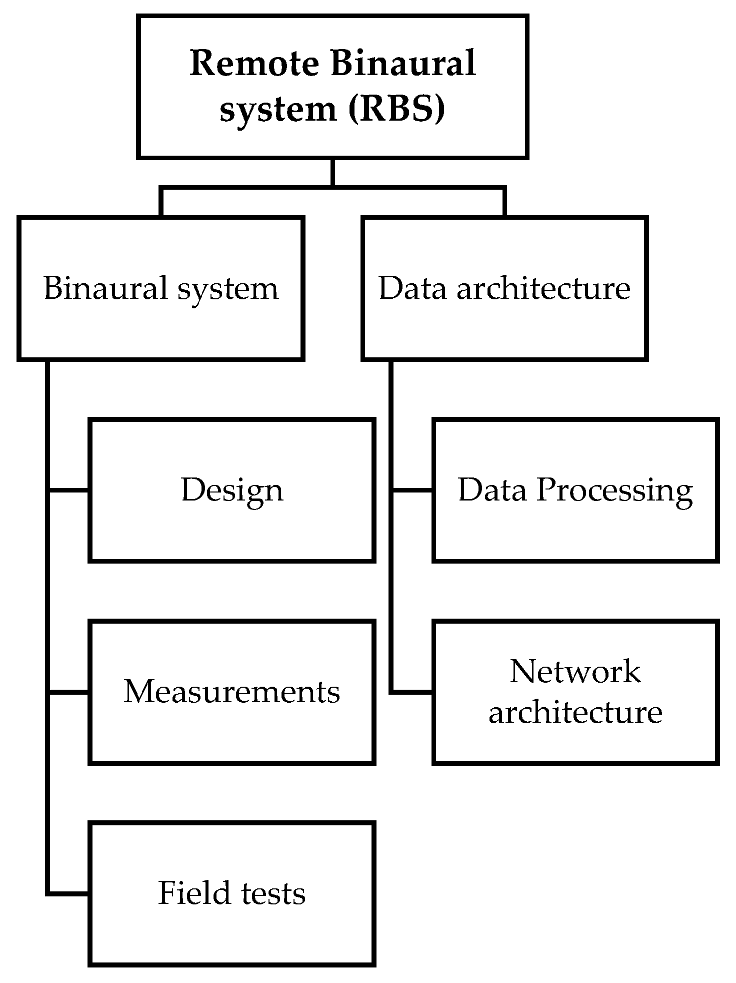
2. Materials and Methods

This section describes the criteria for the design and implementation of the monitoring system prototype, as well as its characterization with the use of acoustic measurements. Two main parts are described. First, the binaural data sensing involves the artificial head with microphones. Second, the software and architecture to receive and process data from the sensors on the cloud. Figure 1 presents both processes.

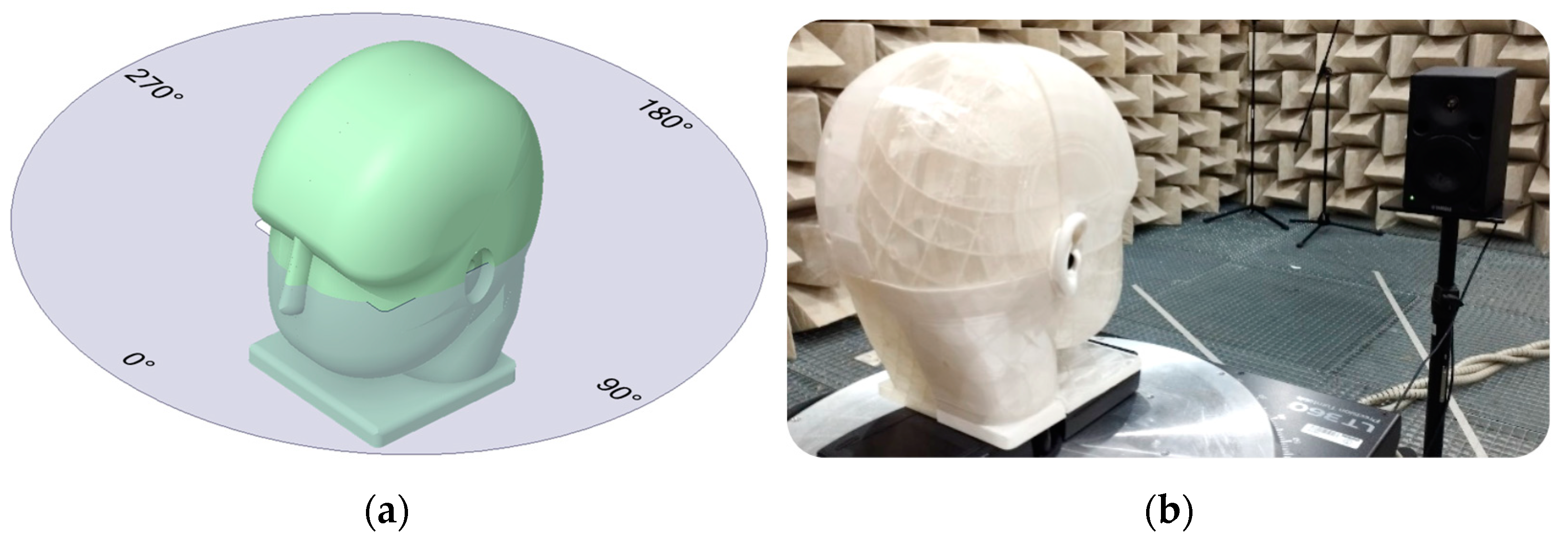
2.1. Artificial Head

2.1.1. Design

When it comes to a binaural audio recording, there are several options documented in the literature and commercial solutions [24,25,26]. As the general idea behind the project was to implement a network of binaural monitoring at several points, commercial heads were not considered due to the costs associated with its installation and operation.

The first approach considered was to use two microphones inside an artificial pinna, each covered using a circle of wood, as shown in Figure 2. Likewise, the small circles in the system were kept in order to hold the silicone artificial pinna. The square box under the microphones was designed to store the electrical parts of the prototype.

The final prototype design was made in CAD software (ANSYS SpaceClaim 2019 R2), seeking to maintain the proportions of an average adult human head. Additionally, in the internal part, the adjustment was made to be able to introduce two microphones. The space for the pinna was covered with two life-size silicone ears. The final design with lateral and 3D views can be seen in Figure 3.

The created model was 3D printed using 1.75 mm PLA (Polylactic acid) material at a temperature of 200 °C. Approximately 1200 g were used with a fill percentage of 9%. This percentage was chosen to make the part lighter and thus facilitate transport and on-site implementation, as well as reduce costs for its serial production. The printing time was approximately two days, and due to its dimensions, which exceeded the capacity of the printer, it was divided into eight sections (four on the front and four on the back). Figure 4b shows the printing result. Future versions may consider larger fills and the printing of only two pieces.

On the other hand, the capture of the acoustic signals was carried out using two omnidirectional condenser acoustic measurement microphones (their frequency response will be shown later). These were connected to a Steinberg UR242 audio interface to carry out the respective digitization and transmission to a PC. The selection of analog and non-digital microphones was determined using the randomness of the lag produced by them when making simultaneous captures, which affected the obtaining of the spatial parameters.

2.1.2. Anechoic Chamber Measurements

The measurements were made in the anechoic chamber of the Polytechnic University of Madrid. Pink noise was used as the excitation signal, guaranteeing a signal-to-noise ratio of 25 dB for all frequency bands. The prototype was placed on a remotely controlled turntable from another room, allowing values to be obtained for different degrees of analysis. Only azimuthal variations were considered. Figure 4a shows the measurement plane in the counterclockwise direction and the experimental setup. The position of the source never changed during the experiment.

The source used was a two-way Yamaha MSP5 Studio active loudspeaker with a frequency response from 50 Hz to 40 kHz. All optional settings included in this speaker have been disabled. The microphones were calibrated at 1 kHz and 94 dB before starting the measurement. The excitation signal was a sine sweep, taking three repetitions per point and obtaining results per 1/3 octave band from 100 Hz to 16,000 Hz. This bandwidth was defined based on IEC 60318-7 [27]. Likewise, the FRF (Frequency response function) of the microphones used in the prototype was adjusted by compensating for the response of the loudspeaker used as an acoustic source. The above is in such a way that only the effect of the head and pinna is reflected.

2.1.3. Field Measurements

In this section, two devices were used: the monitoring station prototype and a class 1 sound level meter. The purpose of using the sound level meter (SLM) was to compare the results of Leq, LAeq, and levels per third of an octave obtained using both measurement systems. It is known that the effect of the head in binaural listening affects the frequency response for each ear differently depending on the angle of incidence of the sound source [28], so differences are expected between the measurement with the microphone of the omnidirectional flat response of the microphone and the measurement microphones implemented in the binaural head of the station. Hence, energetic values obtained are used only as a reference.

A 15-minute continuous measurement was performed as a “baseline” with both devices at a height of 1.5 m (Figure 5a). Likewise, both were calibrated using a class 1 pistonphone (94 dB at 1 kHz) before and after the procedure. A point located on a main street in Bogotá–Colombia was taken as the measurement location. Figure 5b shows the point in the geodetic coordinate system EPSG:4686. This is an important avenue through which heavy vehicles, public transport, motorcycles, and private vehicles pass. Likewise, through the bike path located in the middle of the road, there is traffic of bicycles and other motorized personal transport vehicles. Additionally, there is a traffic light on the road on the east–west side, although this did not generate a concentration of vehicles near the measurement position. As mentioned, during the measurement time, the predominant noise source was road traffic. The circulation speed was close to 45 km/h, so the contribution of the powertrain predominated and, to a lesser extent, road noise, resulting in a low-frequency noise source. There were conditions of dry pavement and fluid circulation of vehicles. Finally, the distance from the measurement point to the buildings was greater than 50 m, decreasing the influence of lateral reflections.

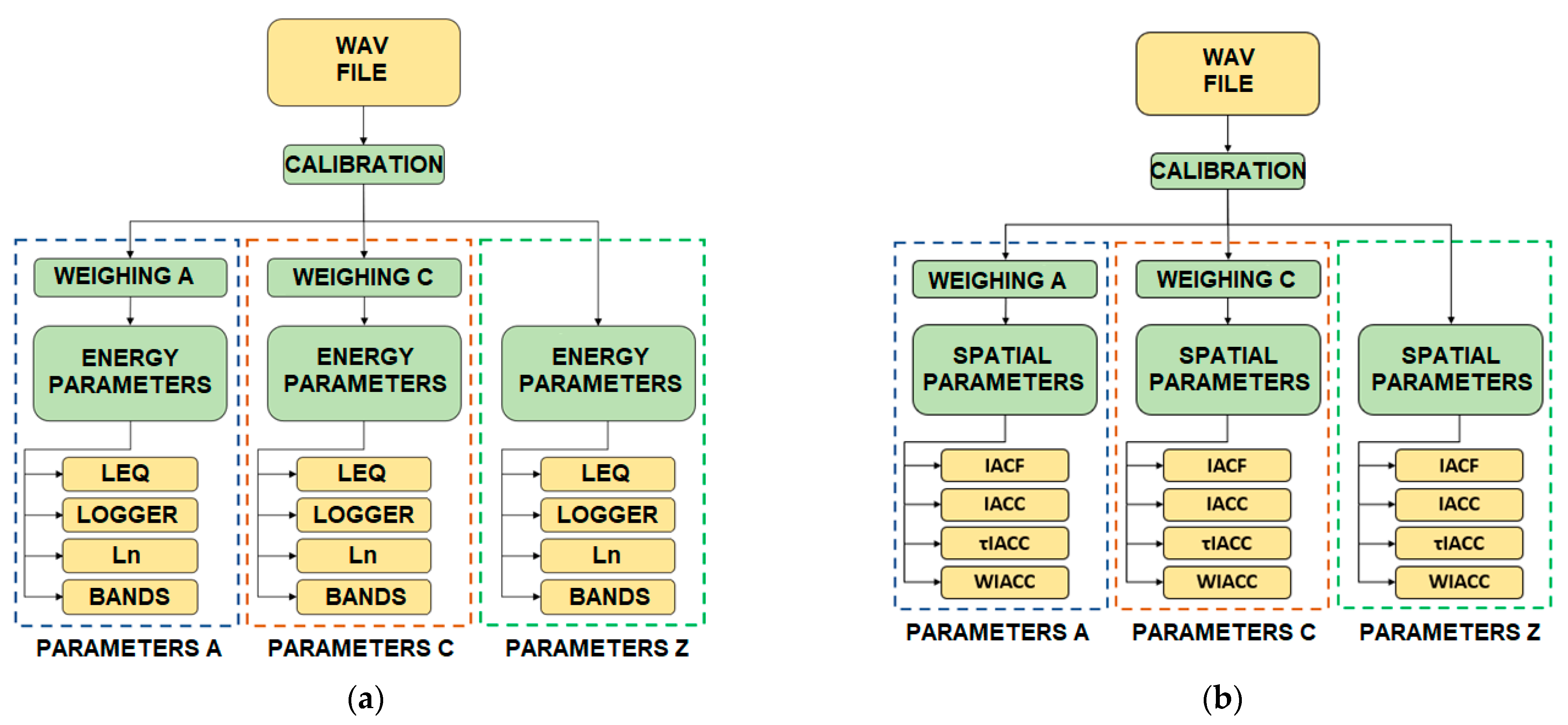
2.2. Data Processing

2.2.1. Acoustic Parameter Software

Besides the hardware, the prototype development includes the software dedicated to the obtention of the energetic and spatial acoustic indicators. This will be described in detail in each of the following aspects.

To obtain the energetic acoustic indicators, a class was developed that receives the arrangement with the audio samples, the sampling frequency, and the type of weighting to be applied. Figure 6a shows the structure of the program. In this case, three instances of the time parameters class are created, each with a different weight.

On the other hand, spatial acoustic indicators were obtained using an algorithm that computed the IACF by applying autocorrelation and normalized cross-correlation equations. The calculations of the spatial parameters made with the algorithm were compared with the results of the analysis using the DSSF3 software (version 5), validating the correct functioning of the developed algorithms. Figure 6b shows the scheme of the developed program.

• Autocorrelation Function

Correlation allows statistical analysis of the linear relationship between two variables. When there is a signal in the time domain, it is characterized by having a periodicity. Using the autocorrelation function (ACF), it is possible to measure the correlation of a signal with itself in versions displaced in time. Depending on the type of signal, the ACF may have different periodic and/or random components. The normalized autocorrelation function (NACF) has been proposed as a sound quality analysis tool [29]. This analysis establishes a window size, a running step to scroll the analysis window, and a running time τ that defines the window delay for the correlation calculation. The ACF is normalized by dividing the geometric average between the energy of the original window and that of the time-shifted window.

• Interaural Cross-Correlation

Cross-correlation (CCF) performs the process of correlating between two different signals. In this case, interaural cross-correlation (IACF) analyzes the left and right channels of a binaural recording [30]. The displacement time of the right channel with respect to the left τ has a range of −1 ms to 1 ms due to the maximum interaural time difference between the two ears of a human head. The IACC of the window is the maximum value that is obtained from the IACF, and τIACC is the value of τ at which the IACC is found. WIACC is the time difference between the two points close to the IACC, at which it falls by 90%.

2.2.2. Network Architecture for Cloud Storage and Processing

The main challenge of this project was to develop an architecture that could support more than 12 sound monitor stations, each transmitting approximately 288 sound events per day and processing each sound file with an average size of 80 MB. Since the algorithms could change in the future and the number of stations could increase, we opted to use an event-driven architecture as described by Michelson [31]. This type of architecture is inherently loosely coupled and highly distributed, which makes it easy to maintain and scale the solution in the long run.

While using a device with the capacity to perform sound processing is a viable approach, it may not always be the optimal solution. Sometimes, the algorithms used for sound processing can be complex and resource-intensive, and introducing new features could further strain the device’s resources, ultimately increasing the cost of implementation. Considering the potential resource limitations of on-site devices, we decided to adopt an on-cloud processing approach while designing the system architecture. This approach allows us to leverage the scalability and flexibility of cloud resources, ensuring that we can handle the processing requirements of our system effectively, even as they evolve over time.

As illustrated in Figure 7, the architecture of our system is based on an event-driven design. We have deployed two applications in AWS Beanstalk as worker agents, which receive messages from the Simple Queue Service (SQS). The SQS, in turn, receives notifications from the Simple Notification Service (SNS) whenever an audio file -in WAV format- is uploaded to the S3 bucket named “soundmonitor-audiodata”. We identified the following advantages of this type of design.

• One of the key benefits of using the event-driven architecture on AWS Beanstalk is the scalability it provides. We can easily increase the number of worker agents taking messages from the SQS service to handle additional loads as needed.
• If a new algorithm is developed in the future, it can be integrated into the system without major changes to the overall architecture by adding a new Beanstalk agent and including a new subscriber to the SNS service, allowing for efficient and flexible updates.
• AWS Beanstalk allows for vertical scalability, meaning that if any of the current or future algorithms used for processing require more computing resources, we can easily increase the resources at any time.
• The results from the algorithms are stored in JSON format in the “soundmonitor-NoiseLevel” and “soundmonitor-NoiseType” S3 buckets, enabling the integration between multiple AWS services, such as AWS Quicksight, for visualization purposes.

We opted to use Raspberry Pi devices to collect audio from the recording devices in our sound monitoring stations. However, after an analysis of the required services and resources, it was found that these devices lacked the resources to perform space-time sound metrics calculator algorithms for on-site processing. As a result, we decided to use an on-cloud processing approach, as discussed earlier. This means that the Raspberry Pi devices are only responsible for capturing sounds from the environment around the recording devices and uploading the audio to the cloud via the HTTPS protocol.

3. Results and Discussion

In this section, the results obtained are discussed.

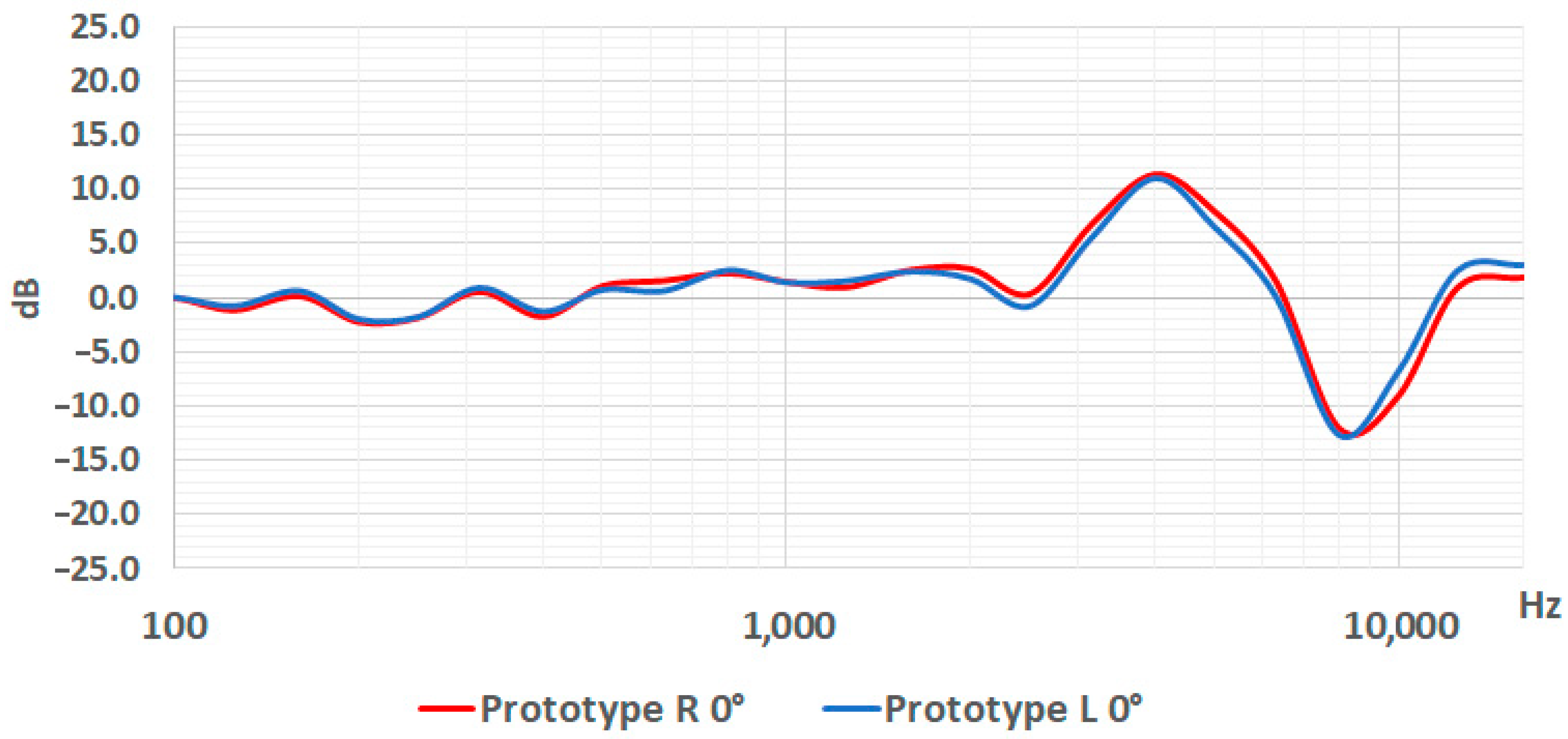
3.1. Anechoic Chamber

Initially, the free field frequency response graphs of the microphones used in the prototype were obtained. In 160 Hz, 250 Hz, and 400 Hz bands, there are increases of approximately +1 dB. Then, from 5000 Hz, there is an ascending behavior up to 16 kHz with a peak value of +6.8 dB. This information was used to apply an inverse filter during prototype data processing.

Data for head-mounted microphones were then processed for a zero-degree angle to the speaker. Figure 8 initially shows how an increase of up to 11 dB is presented at 4 Hz and an attenuation of −13 dB at 8 kHz. This can be attributed to different aspects. Firstly, the microphones are located 2.1 cm inside the prototype, creating a semi-closed tube whose first resonant frequency for ¼ wavelength is approximately 4 kHz. It is worth mentioning that this behavior extends a bit more between 5 kHz and 6 kHz, which may be caused by the shell effect inside the pinnae.

On the other hand, for 1/2 wavelength, there must be attenuation for the semi-closed tube model, which would explain the strong drop at 8 kHz. Then, between 12.5 kHz and 16 kHz, another resonance occurs, mainly associated with the third harmonic of the ear canal. Finally, the differences between the right and left channels can be caused by small differences in the physical shape of the ears used.

In the case of 180°, in general lines, there is a similar frequency behavior up to 2.5 KHz. Then, at the first resonant frequency of the ear canal (4 kHz), there is a difference of approximately 3.5 dB for both channels; however, the trend is maintained up to 8 kHz. From then on, the differences between 0° and 180° are very marked, with values between 4 dB and 14 dB, the latter being evident for frequencies greater than 12 kHz. This could be explained because the incident wavelength begins to be comparable with the size of the pinna and its internal structure. In this way, in practical terms, to discern whether the acoustic source is in front of or behind the prototype, frequencies from 8 kHz onwards play a fundamental role.

In the same way, the analysis was carried out for 90° and 180°, the results of which are shown in Figure 9. It can be observed that the right and left channels follow a similar behavior, presenting higher amplitudes when the source is in front of the prototype’s ears (R 90° and L 270°). For the opposite case (R 270° and L 90°), there are greater differences between each ear; however, the trend remains.

In a complementary way, the frequency response data of the prototype were compared with the Head Acoustics HMS II.3 binaural head. Figure 10 shows the results of a single channel for four angles of incidence of the acoustic wavefront in the direct field. The values used for comparison were obtained in the same anechoic chamber under the same previously mentioned methodology.

In all four incidence angles studied, the HMS II system presents greater amplitude at all frequencies, as well as a more linear behavior at low frequencies. On the other hand, the HMS II shows amplification between 2 kHz and 5 Hz for 0° and 180°, while in the case of the prototype, its response is narrow, focusing on 3 kHz. Likewise, the differences between the prototype and the commercial head can be explained from different perspectives. For example, with respect to resonant frequencies and frequency response, the commercial head must have ear simulators that comply with IEC 60318-4, and all together must comply with IEC 60318-7. This series of standards specifies the impedance and frequency response that must be met. All of the above is because the commercial head focuses mainly on standard measurements in closed spaces. In the case of the prototype, a design was made where the main objective is to obtain a binaural record without the costs of a commercial head and become a first step for binaural acoustic monitoring. In this way, the differences in the technical characteristics of the transducers and the use of normalized pinnas in the commercial head directly influence the variances in FRF. On the other hand, as mentioned above, the distance to the ear canal of the prototype and the materials are also the cause of the differences between the FRF of the prototype and the commercial head.

Finally, the results are presented after applying the correlation functions to obtain the IACF and the spatial acoustic indicators for 0°, 90°, 180° and 270° (Figure 11). During this experiment, the source remained fixed by only varying the position of the prototype on the azimuthal axis and emitting a broadband noise for 30 s.

The τIACC values showed consistency when comparing the position of the source with respect to the prototype. Thus, for 90° and 270°, τIACC was −0.79 ms and 0.78 ms, respectively. It is worth mentioning that this indicator is directly related to the ITD (interaural time difference) and, therefore, makes sense for angles other than 0° and 180°. Similarly, the τIACC values for 90° and 270° are within the limits of an IACF function and are close to the maximum ITD of a typical human head (0.66 mS) [32].

In the cases of incidence under 0° and 180°, amplitudes close to 1 are presented in the IACC value, indicating high similarity for the two ears, as expected. Although the graphs of the IACF function are very similar, the differences are found in the presence of some additional peaks at the extremes, possibly caused by differences between the FRFs of both ears. Finally, ωIACC in all cases was 0.03 for the four source positions, and there was a sharp peak of the IACF. This means that by placing the source on the horizontal plane, there will be a well-defined localization [33].

3.2. Field Measurements

These measurements sought to characterize the behavior of the prototype in a space close to its final application. Next, the results of the energetic and spatial acoustic indicators obtained with the open space prototype are presented.

3.2.1. Energetic Parameters

Table 1. Equivalent continuous level results were obtained with the sound level meter (SVAN 977) and the station head for both channels (RBS L and RBS R).

	Measurements			Differences
	SVAN 977	RBS L	RBS R	RBS L SVAN	RBS R SVAN
Leq A	68.1	71.3	71.8	3.2	3.7
Leq C	79.1	81.6	82.5	2.5	3.4
Leq Z	82.0	83.1	84.1	1.1	2.1

shows the results for the equivalent continuous level. It is observed that the head measured higher levels than those obtained using the sound level meter. The biggest differences are found in the A-weighting (3.2 dB in the right channel and 3.7 dB in the left channel), while the Z-weighting presents the smallest differences (1.1 dB in the right channel and 2.1 dB in the left channel).

Figure 12 shows the levels obtained using third-octave bands. The smallest differences obtained between the head and the sound level meter are found in the band range between 80 Hz and 500 Hz (less than ±1.0 dB). Starting at 2 kHz, the effect of the head begins to generate attenuation in the ear opposite to the direction of the sound source or gains in the direct ear. Therefore, the head of the station works according to what is expected to be the effect of a real human head. However, there are differences in low frequency (20 Hz to 60 Hz), which could have been due to the lack of a windscreen on the binaural headset microphones. The wind generates pressure on the microphone diaphragm intermittently, associated with a low-frequency stimulus. A head gain is also observed with respect to the sound level meter between 2.5 kHz and 8 kHz. In this range, there is the effect of the pinna of the external ear, as well as of the auditory canal, which, due to its physical properties, obtains a resonance at these frequencies. There is a similar effect between 10 kHz and 20 kHz. It is worth noting that an inverse filter was applied to compensate for the head pineapple effect at 0°. However, since the source is road traffic moving from right to left and vice versa and the FRF of the RBS changes for every angle, the increase in energy in the frequencies is still visible, as previously mentioned. Future work will be performed to adapt a windscreen and to find a filter that better compensates for the differences between SLM and the RBS.

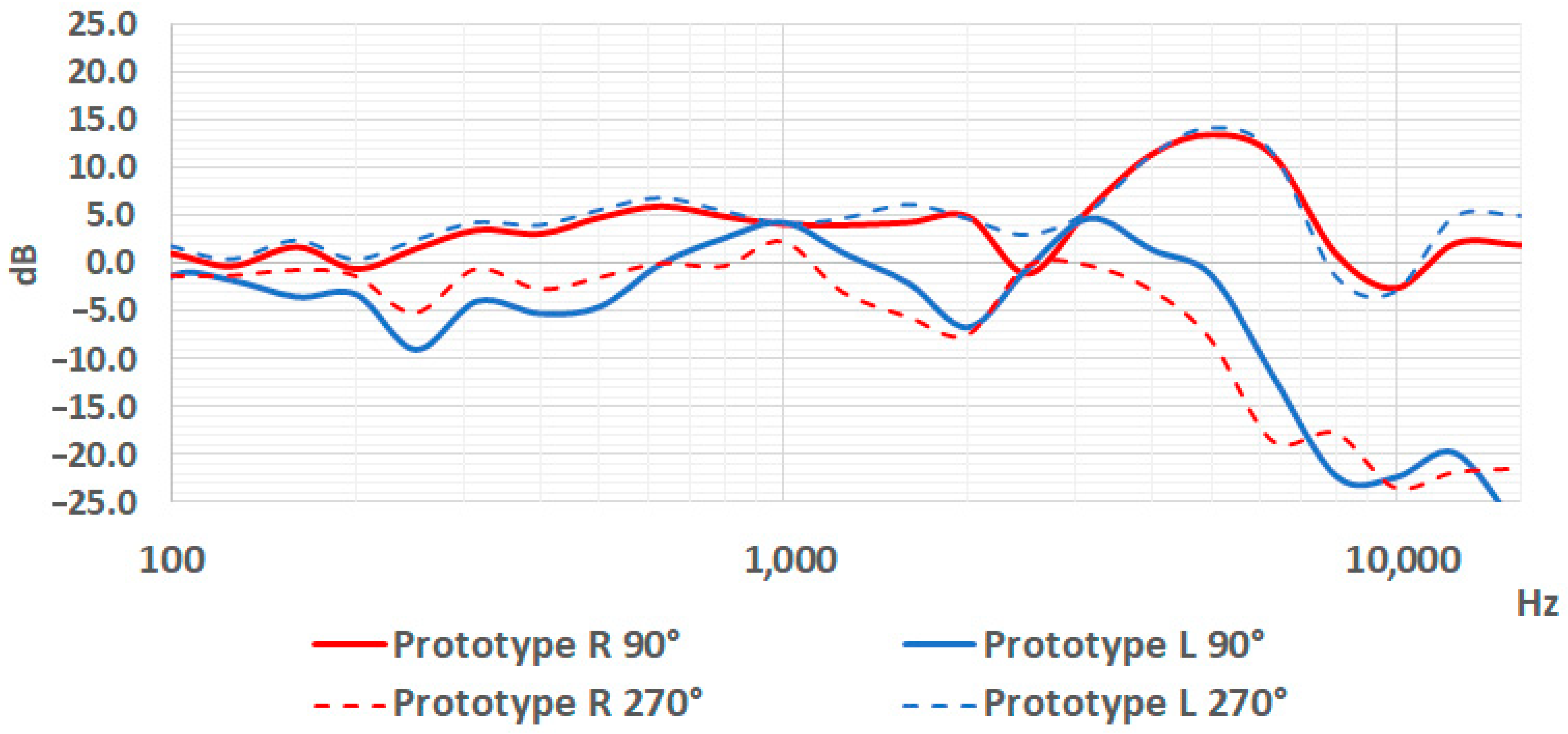
3.2.2. Spatial Parameters

The spatial parameters obtained from the A-weighted IACF are shown in Figure 13. The IACC is a measure of how similar the signals arriving at both ears from the binaural head are. The average value of IACC was 0.2456, with a minimum of 0.0229 and a maximum of 0.8886. Analyzing this function using its percentiles, P10 is 0.1178 and P90 0.4247, with a difference of 0.3069 between them. The difference in these percentiles makes it possible to estimate the variation of the IACC over time. Therefore, there was little correlation between both channels of the recording, being a very diffuse environment.

The τIACC makes it possible to obtain the temporal difference between both ears over time. This function shows a P10 of −0.7708 and a P90 of −0.7917, having a high difference between them, which suggests that there was a high variation of the different sound sources during the recording. This is due to the traffic that was passing through Calle 170 during the recording. The difference between these τIACC percentiles is inversely proportional to the overall perceived quality of the sound environment.

WIACC is an indicator of the apparent width of the sound source, which is inversely dependent on frequency. The P10 had a value of 0.0854 and the P90 of 0.2511. There are peaks in the WIACC graph, which can be associated with sound events of short duration and with predominantly low-frequency content.

4. Future Work

Currently, work is being performed on the development of the other stations in order to integrate them into the capture and processing architecture deployed in AWS. Likewise, the classification of sound sources using AI is being deepened with the aim of knowing more information about the sound landscape of each point where the stations are located. Another approach that is being explored is to have stations with the possibility of performing Edge Computing for those cases in which broadband internet access is not possible. Finally, the main objective of the project is to provide state entities and research groups with useful data to implement urban planning policies that improve the quality of life of citizens.

5. Conclusions

A prototype of a binaural acoustic monitoring system was implemented using the shape of a 3D-printed human head as a design basis. Measurements carried out in an anechoic chamber allowed obtaining the FRF at four different angles, showing variations in medium and high frequencies caused by the pinna and ear canal effect. These variations, in general terms, follow the trend of a commercial head, however, with displacements in frequency and amplitude around 4 kHz. The above could be improved by increasing the distance between the microphones and the exterior ear, which leads to adjusting the physical design of the head. Regarding the spatial location of the source based on the IACF function, the difference between 90° and 270° was clear. However, for 0° and 180°, the similarity of τIACC made this task difficult.

Additionally, a measurement was made on the field to compare the results of the temporal acoustic parameters with a sound level meter class 1. The prototype simulates the effect of a human head in binaural listening, generating interaural differences using bands. The head effect causes certain frequency ranges to be boosted or attenuated, depending on the angle of incidence of the source, as described in Figure 12. In general, for the measurements made, the station shows equivalent continuous level values greater than those of the sound level meter for each of the weights measured. The main goal of the station is to obtain spatial indicators; however, a single microphone class 1 could be attached to obtain more accurate results, like a sound level meter. Regarding the spatial parameters, it was observed that the prototype can provide them once the data is transmitted and processed on the cloud. This is useful to obtain additional data that can help to apply new approaches in soundscape evaluation in urban scenarios.

References

1. Department of Economic and Social Affairs. Population 2030: Demographic Challenges and Opportunities for Sustainable Development Planning; United Nations: New York, NY, USA, 2015; Volume 58.
2. Clark, C. Systematic Review of Evidence on the Effect of Environmental Noise on Quality of Life, Wellbeing and Mental Health. In Proceedings of the INTER-NOISE and NOISE-CON Congress and Conference Proceedings, Hamburg, Germany, 21–24 August 2016; Volume 253, pp. 3835–3841. [Google Scholar]
3. Ouis, D. Annoyance from Road Traffic Noise: A Review. J. Environ. Psychol. 2001, 21, 101–120. [Google Scholar] [CrossRef]
4. Starke, K.R.; Schubert, M.; Kaboth, P.; Gerlach, J.; Hegewald, J.; Reusche, M.; Friedemann, D.; Zülke, A.; Riedel-Heller, S.G.; Zeeb, H.; et al. Traffic Noise Annoyance in the LIFE-Adult Study in Germany: Exposure-Response Relationships and a Comparison to the WHO Curves. Environ. Res. 2023, 228, 115815. [Google Scholar] [CrossRef] [PubMed]
5. Yang, M.; Masullo, M. Combining Binaural Psychoacoustic Characteristics for Emotional Evaluations of Acoustic Environments. Appl. Acoust. 2023, 210, 109433. [Google Scholar] [CrossRef]
6. Sun, K.; De Coensel, B.; Filipan, K.; Aletta, F.; Van Renterghem, T.; De Pessemier, T.; Joseph, W.; Botteldooren, D. Classification of Soundscapes of Urban Public Open Spaces. Landsc. Urban Plan. 2019, 189, 139–155. [Google Scholar] [CrossRef] [Green Version]
7. Schulte-Fortkamp, B. Soundscape, Standardization, and Application. In Proceedings of the Euronoise 2018-Conference proceedings, Crete, Greece, 27–31 May 2018; pp. 2445–2450. [Google Scholar]
8. Jeon, J.Y.; Hong, J.Y. Classification of Urban Park Soundscapes through Perceptions of the Acoustical Environments. Landsc. Urban Plan. 2015, 141, 100–111. [Google Scholar] [CrossRef]
9. Jo, H.I.; Jeon, J.Y. Urban Soundscape Categorization Based on Individual Recognition, Perception, and Assessment of Sound Environments. Landsc. Urban Plan. 2021, 216, 104241. [Google Scholar] [CrossRef]
10. Brown, A.L. Soundscape Planning as a Complement to Environmental Noise Management. In INTER-NOISE and NOISE-CON Congress and Conference Proceedings; Institute of Noise Control Engineering: Reston, VA, USA, 2014; Volume 249, pp. 5894–5903. [Google Scholar]
11. Lavia, L.; Dixon, M.; Witchel, H.J.; Goldsmith, M. Applied Soundscape Practices. Soundscape Built Environ. 2016, 10, 243–301. [Google Scholar]
12. Blauert, J.; Jekosch, U. Sound-Quality Evaluation—A Multi-Layered Problem. Acta Acust. United Acust. 1997, 83, 747–753. [Google Scholar]
13. I.S.O. 12913-1: 2014; Acoustics—Soundscape Part 1: Definition and Conceptual Framework. ISO: Geneva, Switzerland, 2014.
14. Genuit, K. A Special Calibratable Artificial-Head-Measurement-System for Subjective and Objective Classification of Noise. In Proceedings of the 1986 international conference on noise control engineering, Cambridge, MA, USA, 21–23 July 1986; pp. 1313–1318. [Google Scholar]
15. Daniel, P.; Fastl, H.; Fedtke, T.; Genuit, K.; Grabsch, H.-P.; Niederdränk, T.; Schmitz, A.; Vorländer, M.; Zollner, M. Kunstkopftechnik-Eine Bestandsaufnahme. In Proceedings of the ACUSTProc. International Congress on Acoustics ICA/Acta Acustica/Nuntius Acusticus, Madrid, Spain, 2–7 September 2007; Volume 93, p. 58. [Google Scholar]
16. ASA—ANSI/ASA S3.19; Method for the Measurement of Real-Ear Protection of Hearing Protectors and Physical Attenuation of Earmuffs. Acoustical Society of America: Melville, NY, USA, 1974.
17. Liu, X.; Song, H.; Zhong, X. A Hybrid Algorithm for Predicting Median-Plane Head-Related Transfer Functions from Anthropometric Measurements. Appl. Sci. 2019, 9, 2323. [Google Scholar] [CrossRef] [Green Version]
18. Schmitz, A. Ein Neues Digitales Kunstkopfmeßsystem. Acta Acust. United Acust. 1995, 81, 416–420. [Google Scholar]
19. Minnaar, P.; Olesen, S.K.; Christensen, F.; Møller, H. Localization with Binaural Recordings from Artificial and Human Heads. J. Audio Eng. Soc. 2001, 49, 323–336. [Google Scholar]
20. Noriega-Linares, J.E.; Rodriguez-Mayol, A.; Cobos, M.; Segura-Garcia, J.; Felici-Castell, S.; Navarro, J.M. A Wireless Acoustic Array System for Binaural Loudness Evaluation in Cities. IEEE Sens. J. 2017, 17, 7043–7052. [Google Scholar] [CrossRef]
21. Segura-Garcia, J.; Navarro-Ruiz, J.M.; Perez-Solano, J.J.; Montoya-Belmonte, J.; Felici-Castell, S.; Cobos, M.; Torres-Aranda, A.M. Spatio-Temporal Analysis of Urban Acoustic Environments with Binaural Psycho-Acoustical Considerations for IoT-Based Applications. Sensors 2018, 18, 690. [Google Scholar] [CrossRef] [PubMed] [Green Version]
22. IEC 60318; Electroacoustics—Simulators of Human Head and Ear—Part 8: Acoustic Coupler for High-Frequency Measurements of Hearing Aids and Earphones Coupled to the Ear by Means of Ear Inserts. International Electrotechnical Commission: Geneva, Switzerland, 2022.
23. IEC 61672-1; Electroacoustics—Sound Level Meters—Part 1: Specifications. International Electrotechnical Commission: Geneva, Switzerland, 2013.
24. O’Connor, D.; Kennedy, J. An Evaluation of 3D Printing for the Manufacture of a Binaural Recording Device. Appl. Acoust. 2021, 171, 107610. [Google Scholar] [CrossRef]
25. Snaidero, T.; Jacobsen, F.; Buchholz, J. Measuring HRTFs of Brüel & Kjær Type 4128-C, GRAS KEMAR Type 45BM, and Head Acoustics HMS II. 3 Head and Torso Simulators; Technical University of Denmark, Department of Electrical Engineering: Lyngby, Denmark, 2011. [Google Scholar]
26. 3Dio 3Dio. Available online: https://3diosound.com/ (accessed on 31 July 2023).
27. IEC 60318-7; Electroacoustics—Simulators of Human Head and Ear—Part 7: Head and Torso Simulator for the Measurement of Sound Sources Close to the Ear. International Electrotechnical Commission: Geneva, Switzerland, 2022.
28. Blauert, J. The Technology of Binaural Listening; Springer: Berlin/Heidelberg, Germany, 2013. [Google Scholar]
29. Fujii, K.; Soeta, Y.; Ando, Y. Acoustical Properties of Aircraft Noise Measured by Temporal and Spatial Factors. J. Sound Vib. 2001, 241, 69–78. [Google Scholar] [CrossRef]
30. Ando, Y.; Cariani, P. Auditory and Visual Sensations; Springer: Berlin/Heidelberg, Germany, 2009. [Google Scholar]
31. Michelson, B.M. Event-Driven Architecture Overview; Patricia Seybold Group: Boston, MA, USA, 2006. [Google Scholar]
32. Wang, D.; Brown, G.J. Computational Auditory Scene Analysis: Principles, Algorithms, and Applications; Wiley-IEEE Press: Hoboken, NJ, USA, 2006. [Google Scholar]
33. Soeta, Y.; Ando, Y. Neurally Based Measurement and Evaluation of Environmental Noise; Springer: Berlin/Heidelberg, Germany, 2015. [Google Scholar]
Figure 1. Development stages of the Remote Binaural system (RBS).
Jsan 12 00063 g001
Figure 2. A first approach of the Binaural Remote system.
Jsan 12 00063 g002
Figure 3. CAD schematic of RBS: (a) 3D View. (b) Internal location of microphones.
Jsan 12 00063 g003
Figure 4. Measurement plane and experimental assembling: (a) Measurement angles; (b) Prototype in anechoic chamber.
Jsan 12 00063 g004
Figure 5. Field measurements. (a) Measurement point. (b) Sound level meter and noise monitoring system prototype station located on a main street.
Jsan 12 00063 g005
Figure 6. Software structure for the obtention of noise indicators: (a) Energetic parameter; (b) Spatial parameters.
Jsan 12 00063 g006
Figure 7. System architecture of the RBS in AWS.
Jsan 12 00063 g007
Figure 8. Comparison of the FRF of the free field prototype for 0° y 180° incidence.
Jsan 12 00063 g008
Figure 9. Comparison of the FRF of the free field prototype for 90° and 270° incidence.
Jsan 12 00063 g009
Figure 10. Comparison of the FRF of the free field prototype to the Head Acoustics HMS II.3: (a) 0°; (b) 90°; (c) 180°; (d) 270°.
Jsan 12 00063 g010aJsan 12 00063 g010b
Figure 11. IACF function obtained with RBS for: (a) 0°; (b) 90°; (c) 180°; (d) 270°.
Jsan 12 00063 g011aJsan 12 00063 g011b
Figure 12. One-third octave bands obtained in the measurement.
Jsan 12 00063 g012
Figure 13. Spatial parameters obtained with IACF calculation with the monitoring station prototype.
Jsan 12 00063 g013