
Assessment the Impacts of Sea-Level Changes on Mangroves of Ceará-Mirim Estuary, Northeastern Brazil, during the Holocene and Anthropocene
 , , , and
Abstract
:1. Introduction
2. Results
2.1. Vegetation and Geomorphological Units
2.2. Multitemporal Analysis
2.3. Radiocarbon Dates
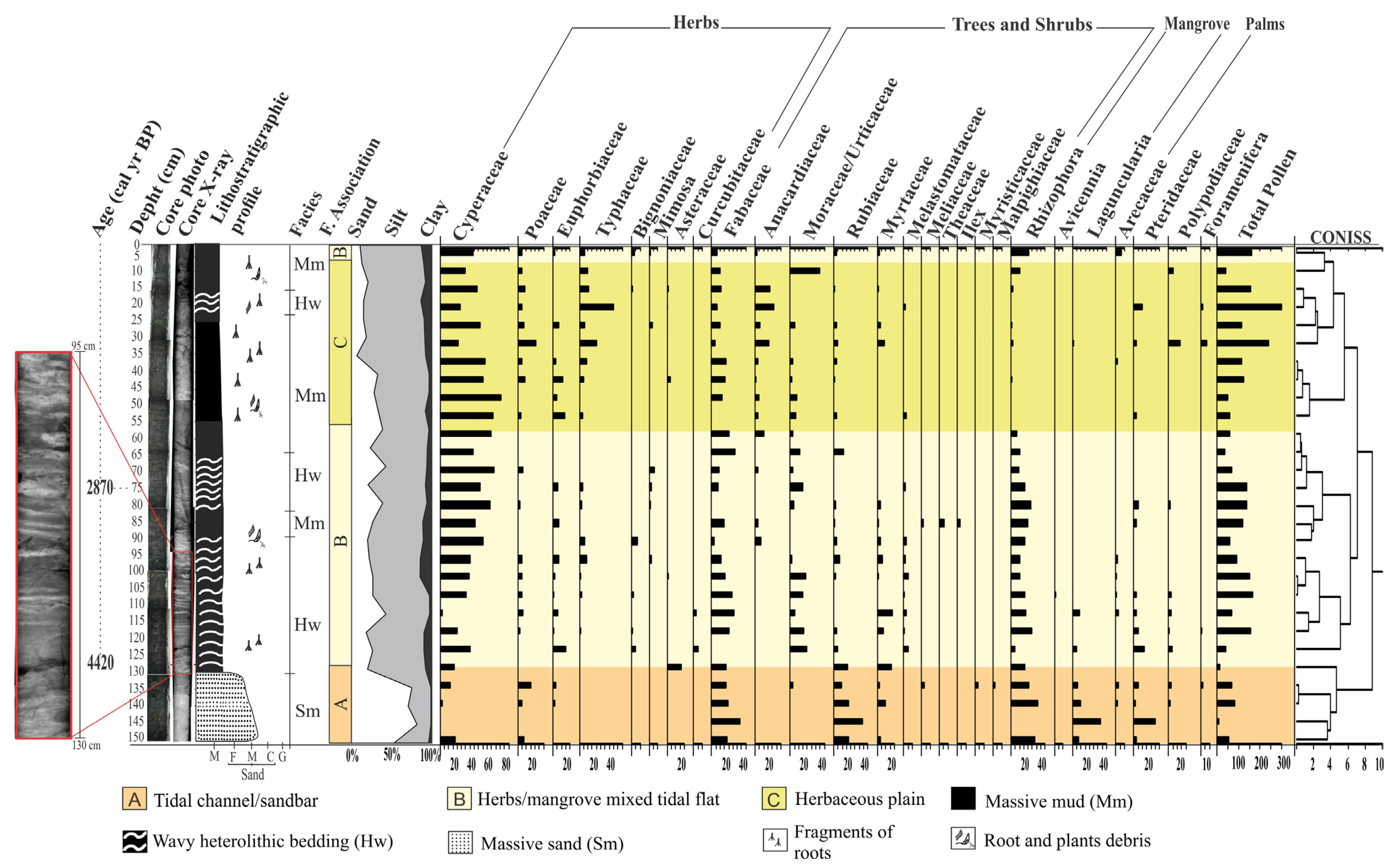
2.4. Facies Description
2.5. Facies Association A (Tidal Channel/Sandbar)
2.6. Facies Association B (Herbs/Mangrove Mixed Tidal Flat)
2.7. Facies Association C (Herbaceous Tidal Flat)
3. Discussion
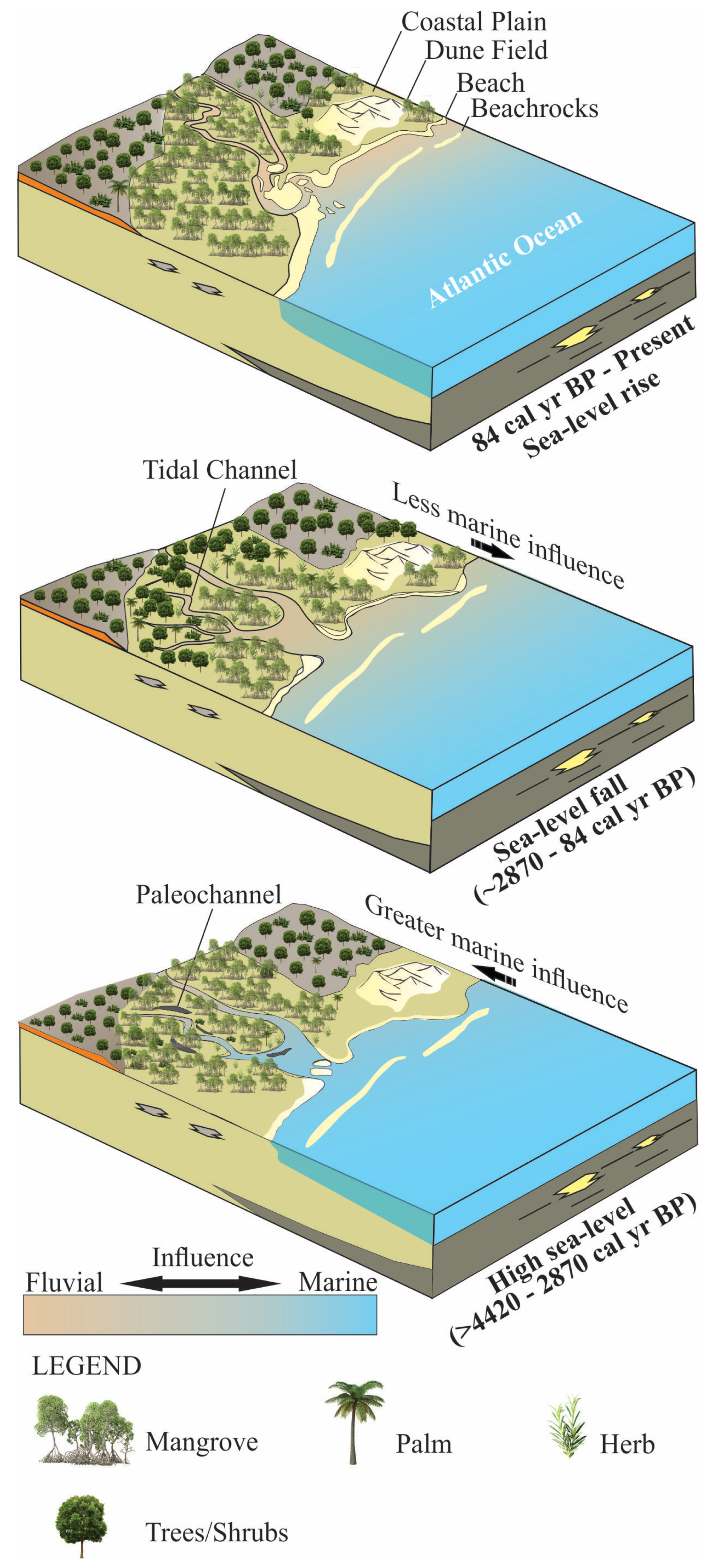
3.1. Depositional Phases
3.2. Mid-Holocene High Sea-Level Stand
3.3. Sea-Level Fall during the Late Holocene
3.4. Climatic Effects
3.5. Recent Sea-Level Rise
4. Materials and Methods
4.1. Study Area
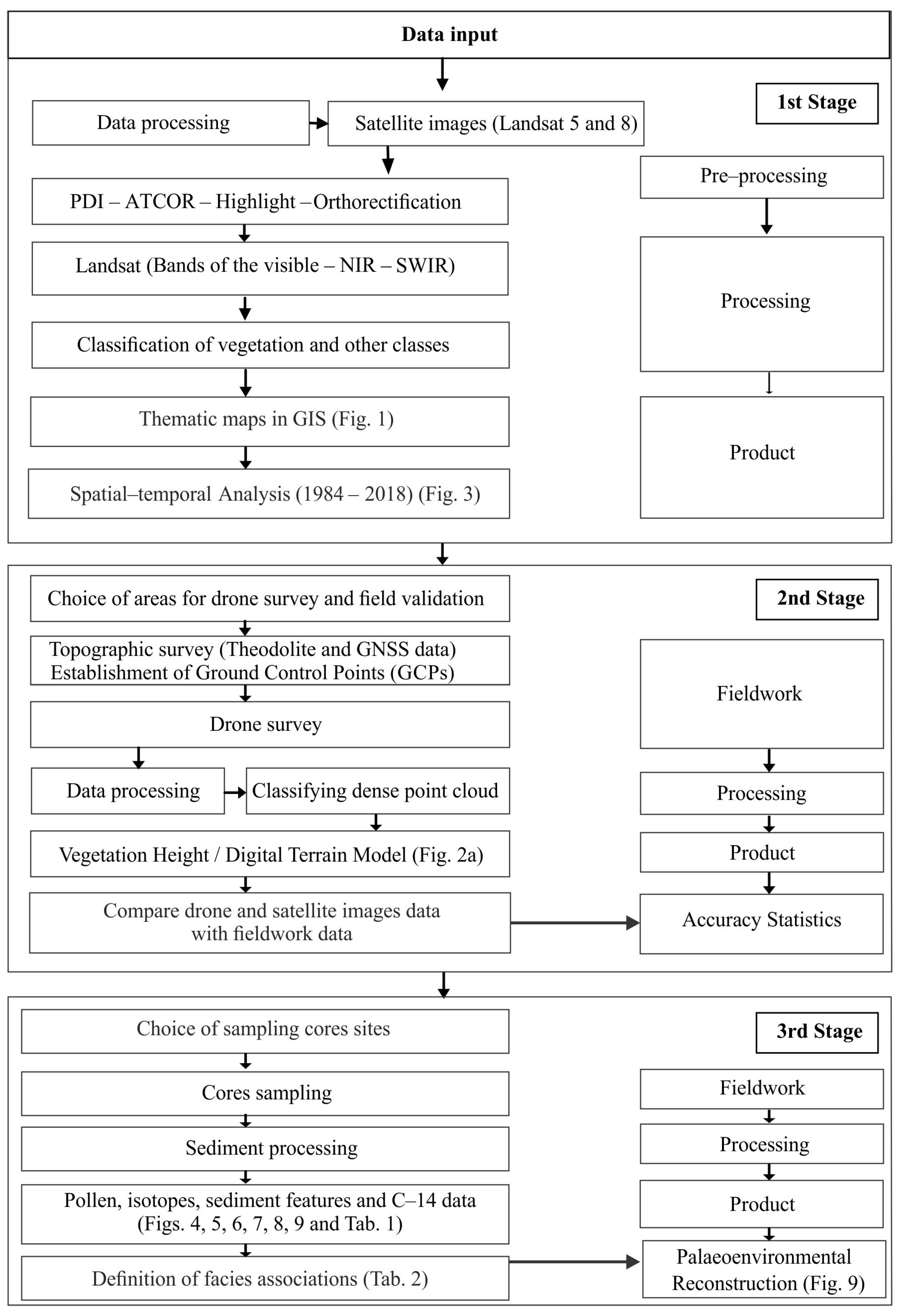
4.2. Remote Sensing
4.3. Topographic and Vegetation Height Models
4.4. Fieldwork and Sample Processing
4.5. Facies Description
4.6. Pollen Analysis
4.7. Isotopic Analysis
4.8. Radiocarbon Dating
5. Conclusions
Supplementary Materials
Author Contributions
Funding
Institutional Review Board Statement
Informed Consent Statement
Data Availability Statement
Acknowledgments
Conflicts of Interest
References
- Cohen, M.C.L.; Rodrigues, E.; Rocha, D.O.S.; Freitas, J.; Fontes, N.A.; Pessenda, L.C.R.; de Souza, A.V.; Gomes, V.L.P.; França, M.C.; Bonotto, D.M.; et al. Southward Migration of the Austral Limit of Mangroves in South America. Catena 2020, 195, 104775. [Google Scholar] [CrossRef]
- Rodrigues, E.; Cohen, M.C.L.; Liu, K.; Pessenda, L.C.R.; Yao, Q.; Ryu, J.; Rossetti, D.; de Souza, A.; Dietz, M. The Effect of Global Warming on the Establishment of Mangroves in Coastal Louisiana during the Holocene. Geomorphology 2021, 381, 107648. [Google Scholar] [CrossRef]
- França, M.C.; Pessenda, L.C.; Cohen, M.C.; de Azevedo, A.Q.; Fontes, N.A.; Silva, F.B.; de Melo, J.C.; de Piccolo, M.C.; Bendassolli, J.A.; Macario, K. Late-Holocene Subtropical Mangrove Dynamics in Response to Climate Change during the Last Millennium. Holocene 2019, 29, 445–456. [Google Scholar] [CrossRef]
- Wolanski, E.; Mazda, Y.; King, B.; Gay, S. Dynamics, Flushing and Trapping in Hinchinbrook Channel, a Giant Mangrove Swamp, Australia. Estuar. Coast. Shelf. Sci. 1990, 31, 555–579. [Google Scholar] [CrossRef]
- Cohen, M.C.L.; Figueiredo, B.L.; Oliveira, N.N.; Fontes, N.A.; França, M.C.; Pessenda, L.C.R.; de Souza, A.V.; Macario, K.; Giannini, P.C.F.; Bendassolli, J.A.; et al. Impacts of Holocene and Modern Sea-Level Changes on Estuarine Mangroves from Northeastern Brazil. Earth Surf. Process. Landf. 2020, 45, 375–392. [Google Scholar] [CrossRef]
- Cohen, M.C.L.; Pessenda, L.C.R.; Behling, H.; de Fátima Rossetti, D.; França, M.C.; Guimarães, J.T.F.; Friaes, Y.; Smith, C.B. Holocene Palaeoenvironmental History of the Amazonian Mangrove Belt. Quat. Sci. Rev. 2012, 55, 50–58. [Google Scholar] [CrossRef]
- Blasco, F.; Saenger, P.; Janodet, E. Mangroves as Indicators of Coastal Change. Catena 1996, 27, 167–178. [Google Scholar] [CrossRef]
- Semeniuk, V. Predicting the Effect of Sea-Level Rise on Mangroves in Northwestern Australia. J. Coast. Res. 1994, 10, 1050–1076. [Google Scholar]
- Cohen, M.C.L.; Camargo, P.M.P.; Pessenda, L.C.R.; Lorente, F.L.; De Souza, A.V.; Corrêa, J.A.M.; Bendassolli, J.; Dietz, M. Effects of the Middle Holocene High Sea-Level Stand and Climate on Amazonian Mangroves. J. Quat. Sci. 2021, 36, 1013–1027. [Google Scholar] [CrossRef]
- Figueiredo, B.L.; Alves, I.C.C.; Cohen, M.C.L.; Pessenda, L.C.R.; França, M.C.; Francisquini, M.I.; de Souza, A.V.; Culligan, N. Climate, Sea-Level, and Anthropogenic Influences on Coastal Vegetation of the Southern Bahia, Northeastern Brazil, during the Mid-Late Holocene. Geomorphology 2021, 394, 107967. [Google Scholar] [CrossRef]
- Cohen, M.C.L.; Behling, H.; Lara, R.J.; Smith, C.B.; Matos, H.R.S.; Vedel, V. Impact of Sea-Level and Climatic Changes on the Amazon Coastal Wetlands during the Late Holocene. Veg. Hist. Archaeobot. 2009, 18, 425–439. [Google Scholar] [CrossRef]
- Cohen, M.C.L.; Behling, H.; Lara, R.J. Amazonian Mangrove Dynamics during the Last Millennium: The Relative Sea-Level and the Little Ice Age. Rev. Palaeobot. Palynol. 2005, 136, 93–108. [Google Scholar] [CrossRef]
- Cohen, M.C.L.; Souza Filho, P.W.M.; Lara, R.J.; Behling, H.; Angulo, R.J. A Model of Holocene Mangrove Development and Relative Sea-Level Changes on the Bragança Peninsula (Northern Brazil). Wetl. Ecol. Manag. 2005, 13, 433–443. [Google Scholar] [CrossRef]
- Bozi, B.S.; Figueiredo, B.L.; Rodrigues, E.; Cohen, M.C.L.; Pessenda, L.C.R.; Alves, E.E.N.; de Souza, A.V.; Bendassolli, J.A.; Macario, K.; Azevedo, P.; et al. Impacts of Sea-Level Changes on Mangroves from Southeastern Brazil during the Holocene and Anthropocene Using a Multi-Proxy Approach. Geomorphology 2021, 390, 107860. [Google Scholar] [CrossRef]
- Lara, R.J.; Cohen, M.C.L. Palaeolimnological Studies and Ancient Maps Confirm Secular Climate Fluctuations in Amazonia. Clim. Chang. 2009, 94, 399–408. [Google Scholar] [CrossRef]
- Angulo, R.J.; Lessa, G.C.; De Souza, M.C. A Critical Review of Mid- to Late-Holocene Sea-Level Fluctuations on the Eastern Brazilian Coastline. Quat. Sci. Rev. 2006, 25, 486–506. [Google Scholar] [CrossRef]
- Lorente, F.L.; Pessenda, L.C.R.; Oboh-Ikuenobe, F.; Buso, A.A.; Cohen, M.C.L.; Meyer, K.E.B.; Giannini, P.C.F.; de Oliveira, P.E.; de Rossetti, D.F.; Borotti Filho, M.A.; et al. Palynofacies and Stable C and N Isotopes of Holocene Sediments from Lake Macuco (Linhares, Espírito Santo, Southeastern Brazil): Depositional Settings and Palaeoenvironmental Evolution. Palaeogeogr. Palaeoclimatol. Palaeoecol. 2014, 415, 69–82. [Google Scholar] [CrossRef]
- de Toniolo, T.F.; Giannini, P.C.F.; Angulo, R.J.; de Souza, M.C.; Pessenda, L.C.R.; Spotorno-Oliveira, P. Sea-Level Fall and Coastal Water Cooling during the Late Holocene in Southeastern Brazil Based on Vermetid Bioconstructions. Mar. Geol. 2020, 428, 106281. [Google Scholar] [CrossRef]
- Martin, L.; Dominguez, J.M.L.; Bittencourt, A.C.S.P. Fluctuating Holocene Sea Levels in Eastern and Southeastern Brazil: Evidence from Multiple Fossil and Geometric Indicators. J. Coast. Res. 2003, 19, 101–124. [Google Scholar]
- Boski, T.; Bezerra, F.H.R.; de Fátima Pereira, L.; Souza, A.M.; Maia, R.P.; Lima-Filho, F.P. Sea-Level Rise since 8.2 Ka Recorded in the Sediments of the Potengi–Jundiai Estuary, NE Brasil. Mar. Geol. 2015, 365, 1–13. [Google Scholar] [CrossRef]
- Fontes, N.A.; Moraes, C.A.; Cohen, M.C.L.; Alves, I.C.C.; França, M.C.; Pessenda, L.C.R.; Francisquini, M.I.; Bendassolli, J.A.; Macario, K.; Mayle, F. The Impacts of the Middle Holocene High Sea-Level Stand and Climatic Changes on Mangroves of the Jucuruçu River, Southern Bahia—Northeastern Brazil. Radiocarbon 2017, 59, 215–230. [Google Scholar] [CrossRef]
- Ribeiro, S.R.; Batista, E.J.L.; Cohen, M.C.L.; França, M.C.; Pessenda, L.C.R.; Fontes, N.A.; Alves, I.C.C.; Bendassolli, J.A. Allogenic and Autogenic Effects on Mangrove Dynamics from the Ceará Mirim River, North-Eastern Brazil, during the Middle and Late Holocene. Earth Surf. Process. Landf. 2018, 43, 1622–1635. [Google Scholar] [CrossRef]
- Thomas, N.; Lucas, R.; Bunting, P.; Hardy, A.; Rosenqvist, A.; Simard, M. Distribution and Drivers of Global Mangrove Forest Change, 1996–2010. PLoS ONE 2017, 12, e0179302. [Google Scholar] [CrossRef] [PubMed]
- Cohen, M.C.L.; Lara, R.J. Temporal Changes of Mangrove Vegetation Boundaries in Amazonia: Application of GIS and Remote Sensing Techniques. Wetl. Ecol. Manag. 2003, 11, 223–231. [Google Scholar] [CrossRef]
- Henrique de Oliveira Caldas, L.; Gomes de Oliveira, J.; Eugênio de Medeiros, W.; Stattegger, K.; Vital, H. Geometry and Evolution of Holocene Transgressive and Regressive Barriers on the Semi-Arid Coast of NE Brazil. Geo-Mar. Lett. 2006, 26, 249–263. [Google Scholar] [CrossRef]
- Cohen, M.C.L.; de Souza, A.V.; Liu, K.-B.; Rodrigues, E.; Yao, Q.; Pessenda, L.C.R.; Rossetti, D.; Ryu, J.; Dietz, M. Effects of Beach Nourishment Project on Coastal Geomorphology and Mangrove Dynamics in Southern Louisiana, USA. Remote Sens. 2021, 13, 2688. [Google Scholar] [CrossRef]
- Hsu, A.J.; Kumagai, J.; Favoretto, F.; Dorian, J.; Martinez, B.G.; Aburto-Oropeza, O. Driven by Drones: Improving Mangrove Extent Maps Using High-Resolution Remote Sensing. Remote Sens. 2020, 12, 3986. [Google Scholar] [CrossRef]
- Yao, Q.; Cohen, M.C.L.; Liu, K.-B.; Vivan De Souza, A.; Rodrigues, E. Nature versus Humans in Coastal Environmental Change: Assessing the Impacts of Hurricanes Zeta and Ida in the Context of Beach Nourishment Projects in the Mississippi River Delta. Remote Sens. 2022, 14, 2598. [Google Scholar] [CrossRef]
- Cohen, M.C.L.; de Souza, A.V.; Liu, K.B.; Rodrigues, E.; Yao, Q.; Ryu, J.; Dietz, M.; Pessenda, L.C.R.; Rossetti, D. Effects of the 2017–2018 Winter Freeze on the Northern Limit of the American Mangroves, Mississippi River Delta Plain. Geomorphology 2021, 394, 107968. [Google Scholar] [CrossRef]
- Cohen, M.C.L.; de Souza, A.V.; Rossetti, D.F.; Pessenda, L.C.R.; França, M.C. Decadal-Scale Dynamics of an Amazonian Mangrove Caused by Climate and Sea Level Changes: Inferences from Spatial–Temporal Analysis and Digital Elevation Models. Earth Surf. Process. Landf. 2018, 43, 2876–2888. [Google Scholar] [CrossRef]
- Andersen, S.T. Tree-Pollen Rain in a Mixed Deciduous Forest in South Jutland (Denmark). Rev. Palaeobot. Palynol. 1967, 3, 267–275. [Google Scholar] [CrossRef]
- Janssen, C.R. Recent Pollen Spectra from the Deciduous and Coniferous-Deciduous Forests of Northeastern Minnesota: A Study in Pollen Dispersal. Ecology 1966, 47, 804–825. [Google Scholar] [CrossRef]
- Sugita, S. Pollen Representation of Vegetation in Quaternary Sediments: Theory and Method in Patchy Vegetation. J. Ecol. 1994, 82, 881. [Google Scholar] [CrossRef]
- Behling, H.; Cohen, M.C.L.; Lara, R.J. Studies on Holocene Mangrove Ecosystem Dynamics of the Bragança Peninsula in North-Eastern Pará, Brazil. Palaeogeogr. Palaeoclimatol. Palaeoecol. 2001, 167, 225–242. [Google Scholar] [CrossRef]
- Davis, M.B. Palynology after Y2K—Understanding the Source Area of Pollen in Sediments. Annu. Rev. Earth Planet. Sci. 2003, 28, 1–18. [Google Scholar] [CrossRef]
- Dittmar, T.; Lara, R.J.; Kattner, G. River or Mangrove? Tracing Major Organic Matter Sources in Tropical Brazilian Coastal Waters. Mar. Chem. 2001, 73, 253–271. [Google Scholar] [CrossRef]
- Dittmar, T.; Hertkorn, N.; Kattner, G.; Lara, R.J. Mangroves, a Major Source of Dissolved Organic Carbon to the Oceans. Glob. Biogeochem. Cycles 2006, 20, GB1012. [Google Scholar] [CrossRef]
- Matos, C.R.L.; Berrêdo, J.F.; Machado, W.; Sanders, C.J.; Metzger, E.; Cohen, M.C.L. Carbon and Nutrient Accumulation in Tropical Mangrove Creeks, Amazon Region. Mar. Geol. 2020, 429, 106317. [Google Scholar] [CrossRef]
- Reading, H.G. Sedimentary Environments Processes, Facies and Stratigraphy; John Wiley & Sons: Hoboken, NJ, USA, 1996; ISBN 8781118687635. [Google Scholar]
- Bradley, R.S. Paleoclimatology: Reconstructing Climates of the Quaternary, 3rd ed.; Elsevier: Amsterdam, The Netherlands, 2014; ISBN 9780123869135. [Google Scholar]
- Ren, G. Some Progresses and Problems in Paloeclimatology. Sci. Geogr. Sin. 1999, 19, 368–378. [Google Scholar]
- Hallett, J. Climate Change 2001: The Scientific Basis. Edited by J. T. Houghton, Y. Ding, D.J. Griggs, N. Noguer, P.J. van Der Linden, D. Xiaosu, K. Maskell and C. A. Johnson. Contribution of Working Group I to the Third Assessment Report of the Intergovernmental Panel on Climate Change, Cambridge University Press, Cambridge. 2001. 881 pp. ISBN 0521 01495 6. Q. J. R. Meteorol. Soc. 2002, 128, 1038–1039. [Google Scholar] [CrossRef]
- Edwards, C.M.; Hodgson, D.M.; Flint, S.S.; Howell, J.A. Contrasting Styles of Shelf Sediment Transport and Deposition in a Ramp Margin Setting Related to Relative Sea-Level Change and Basin Floor Topography, Turonian (Cretaceous) Western Interior of Central Utah, USA. Sediment. Geol. 2005, 179, 117–152. [Google Scholar] [CrossRef]
- Miall, A.D. The Geology of Fluvial Deposits; Springer: Berlin/Heidelberg, Germany, 2006; ISBN 978-3-642-08211-5. [Google Scholar]
- Rossetti, D.F.; Valeriano, M.M.; Góes, A.M.; Thales, M. Palaeodrainage on Marajó Island, Northern Brazil, in Relation to Holocene Relative Sea-Level Dynamics. Holocene 2008, 18, 923–934. [Google Scholar] [CrossRef]
- Rossetti, D.F.; Zani, H.; Cohen, M.C.L.; Cremon, É.H. A Late Pleistocene–Holocene Wetland Megafan in the Brazilian Amazonia. Sediment. Geol. 2012, 282, 276–293. [Google Scholar] [CrossRef]
- Short, A.D. Macro-Meso Tidal Beach Morphodynamics: An Overview. J. Coast. Res. 1991, 7, 417–436. [Google Scholar]
- Meyers, P.A. Applications of Organic Geochemistry to Paleolimnological Reconstructions: A Summary of Examples from the Laurentian Great Lakes. Org. Geochem. 2003, 34, 261–289. [Google Scholar] [CrossRef]
- Peterson, B.J.; Howarth, R.W. Sulfur, Carbon, and Nitrogen Isotopes Used to Trace Organic Matter Flow in the Salt-Marsh Estuaries of Sapelo Island, Georgia1. Limnol. Oceanogr. 1987, 32, 1195–1213. [Google Scholar] [CrossRef]
- Kemp, A.C.; Dutton, A.; Raymo, M.E. Paleo Constraints on Future Sea-Level Rise. Curr. Clim. Chang. Rep. 2015, 1, 205–215. [Google Scholar] [CrossRef]
- Rovere, A.; Stocchi, P.; Vacchi, M. Eustatic and Relative Sea Level Changes. Curr. Clim. Chang. Rep. 2016, 2, 221–231. [Google Scholar] [CrossRef]
- Stronge, W.B.; Diaz, H.F.; Bokuniewicz, H.; Inman, D.L.; Jenkins, S.A.; Hsu, J.R.C.; Kennish, M.J.; Bird, E.; Hesp, P.A.; Crowell, M.; et al. Eustasy. In Encyclopedia of Coastal Science; Springer: Berlin/Heidelberg, Germany, 2005; pp. 439–442. [Google Scholar] [CrossRef]
- Kopp, R.E.; Hay, C.C.; Little, C.M.; Mitrovica, J.X. Geographic Variability of Sea-Level Change. Curr. Clim. Chang. Rep. 2015, 1, 192–204. [Google Scholar] [CrossRef]
- Mitrovica, J.X.; Gomez, N.; Clark, P.U. The Sea-Level Fingerprint of West Antarctic Collapse. Science 2009, 323, 753. [Google Scholar] [CrossRef]
- Dura, T.; Engelhart, S.E.; Vacchi, M.; Horton, B.P.; Kopp, R.E.; Peltier, W.R.; Bradley, S. The Role of Holocene Relative Sea-Level Change in Preserving Records of Subduction Zone Earthquakes. Curr. Clim. Chang. Rep. 2016, 2, 86–100. [Google Scholar] [CrossRef]
- Cohen, M.C.L.; França, M.C.; Rossetti, D.; Pessenda, L.C.R.; Giannini, P.C.F.; Lorente, F.L.; Junior, A.Á.B.; Castro, D.; Macario, K. Landscape Evolution during the Late Quaternary at the Doce River Mouth, Espírito Santo State, Southeastern Brazil. Palaeogeogr. Palaeoclimatol. Palaeoecol. 2014, 415, 48–58. [Google Scholar] [CrossRef]
- Cohen, M.C.L.; Alves, I.C.C.; França, M.C.; Pessenda, L.C.R.; Rossetti, D. de F. Relative Sea-Level and Climatic Changes in the Amazon Littoral during the Last 500 years. Catena 2015, 133, 441–451. [Google Scholar] [CrossRef]
- Lamb, A.L.; Wilson, G.P.; Leng, M.J. A Review of Coastal Palaeoclimate and Relative Sea-Level Reconstructions Using Δ13C and C/N Ratios in Organic Material. Earth Sci. Rev. 2006, 75, 29–57. [Google Scholar] [CrossRef]
- Meyers, P.A. Preservation of Elemental and Isotopic Source Identification of Sedimentary Organic Matter. Chem. Geol. 1994, 114, 289–302. [Google Scholar] [CrossRef]
- Tyson, R.V. Sedimentary Organic Matter. In Sedimentary Organic Matter; Springer: Berlin/Heidelberg, Germany, 1995. [Google Scholar] [CrossRef]
- Wright, I.P. Stable Isotopic Compositions of Hydrogen, Carbon, Nitrogen, Oxygen and Sulfur in Meteoritic Low Temperature Condensates. In Ices in the Solar System; Springer: Berlin/Heidelberg, Germany, 1985; pp. 221–249. [Google Scholar] [CrossRef]
- Deines, P. The Isotopic Composition of Reduced Organic Carbon. In The Terrestrial Environment, A; Elsevier Science: Waterloo, ON, Canada, 1980; Volume 1, pp. 329–406. [Google Scholar]
- Woodroffe, C.D. Mangrove Swamp Stratigraphy and Holocene Transgression, Grand Cayman Island, West Indies. Mar. Geol. 1981, 41, 271–294. [Google Scholar] [CrossRef]
- Bezerra, F.H.R.; Barreto, A.M.F.; Suguio, K. Holocene Sea-Level History on the Rio Grande Do Norte State Coast, Brazil. Mar. Geol. 2003, 196, 73–89. [Google Scholar] [CrossRef]
- Szczygielski, A.; Stattegger, K.; Schwarzer, K.; da Silva, A.G.A.; Vital, H.; Koenig, J. Evolution of the Parnaíba Delta (NE Brazil) during the Late Holocene. Geo-Mar. Lett. 2015, 35, 105–117. [Google Scholar] [CrossRef]
- Khan, N.S.; Ashe, E.; Horton, B.P.; Dutton, A.; Kopp, R.E.; Brocard, G.; Engelhart, S.E.; Hill, D.F.; Peltier, W.R.; Vane, C.H.; et al. Drivers of Holocene Sea-Level Change in the Caribbean. Quat. Sci. Rev. 2017, 155, 13–36. [Google Scholar] [CrossRef]
- Angulo, R.J.; Giannini, P.C.F.; De Souza, M.C.; Lessa, G.C.; Angulo, R.J.; Giannini, P.C.F.; De Souza, M.C.; Lessa, G.C. Holocene Paleo-Sea Level Changes along the Coast of Rio de Janeiro, Southern Brazil: Comment on Castro et al. (2014). An. Acad. Bras. Cienc. 2016, 88, 2105–2111. [Google Scholar] [CrossRef]
- Woodroffe, C.D.; Murray-Wallace, C.V. Sea-Level Rise and Coastal Change: The Past as a Guide to the Future. Quat. Sci. Rev. 2012, 54, 4–11. [Google Scholar] [CrossRef]
- Schwartz, M. Laboratory Study of Sea-Level Rise as a Cause of Shore Erosion. J. Geol. 1965, 73, 528–534. [Google Scholar] [CrossRef]
- Ellison, J.C. Vulnerability Assessment of Mangroves to Climate Change and Sea-Level Rise Impacts. Wetl. Ecol. Manag. 2015, 23, 115–137. [Google Scholar]
- Pessenda, L.C.R.; Ribeiro, A.D.S.; Gouveia, S.E.M.; Aravena, R.; Boulet, R.; Bendassolli, J.A. Vegetation Dynamics during the Late Pleistocene in the Barreirinhas Region, Maranhão State, Northeastern Brazil, Based on Carbon Isotopes in Soil Organic Matter. Quat. Res. 2004, 62, 183–193. [Google Scholar] [CrossRef]
- Freitas, H.A.; Pessenda, L.C.R.; Aravena, R.; Gouveia, S.E.M.; de Souza Ribeiro, A.; Boulet, R. Late Quaternary Vegetation Dynamics in the Southern Amazon Basin Inferred from Carbon Isotopes in Soil Organic Matter. Quat. Res. 2001, 55, 39–46. [Google Scholar] [CrossRef]
- Behling, H.; Hooghiemstra, H. Late Quaternary Palaeoecology and Palaeoclimatology from Pollen Records of the Savannas of the Llanos Orientales in Colombia. Palaeogeogr. Palaeoclimatol. Palaeoecol. 1998, 139, 251–267. [Google Scholar] [CrossRef]
- Ledru, M.-P.; Salatino, M.L.F.; Ceccantini, G.; Salatino, A.; Pinheiro, F.; Pintaud, J.-C. Regional Assessment of the Impact of Climatic Change on the Distribution of a Tropical Conifer in the Lowlands of South America. Divers. Distrib. 2007, 13, 761–771. [Google Scholar] [CrossRef]
- Pessenda, L.C.R.; De Oliveira, P.E.; Mofatto, M.; de Medeiros, V.B.; Francischetti Garcia, R.J.; Aravena, R.; Bendassoli, J.A.; Zuniga Leite, A.; Saad, A.R.; Lincoln Etchebehere, M. The Evolution of a Tropical Rainforest/Grassland Mosaic in Southeastern Brazil since 28,000 14C Yr BP Based on Carbon Isotopes and Pollen Records. Quat. Res. 2009, 71, 437–452. [Google Scholar] [CrossRef]
- Wanner, H.; Beer, J.; Bütikofer, J.; Crowley, T.J.; Cubasch, U.; Flückiger, J.; Goosse, H.; Grosjean, M.; Joos, F.; Kaplan, J.O.; et al. Mid- to Late Holocene Climate Change: An Overview. Quat. Sci. Rev. 2008, 27, 1791–1828. [Google Scholar] [CrossRef]
- Behling, H.; Arz, H.W.; Pätzold, J.; Wefer, G. Late Quaternary Vegetational and Climate Dynamics in Southeastern Brazil, Inferences from Marine Cores GeoB 3229-2 and GeoB 3202-1. Palaeogeogr. Palaeoclimatol. Palaeoecol. 2002, 179, 227–243. [Google Scholar] [CrossRef]
- Behling, H. A High Resolution Holocene Pollen Record from Lago Do Pires, SE Brazil: Vegetation, Climate and Fire History. J. Paleolimnol. 1995, 14, 253–268. [Google Scholar] [CrossRef]
- Behling, H. Investigations into the Late Pleistocene and Holocene History of Vegetation and Climate in Santa Catarina (S Brazil). Veg. Hist. Archaeobot. 1995, 4, 127–152. [Google Scholar] [CrossRef]
- Bernal, J.P.; Cruz, F.W.; Stríkis, N.M.; Wang, X.; Deininger, M.; Catunda, M.C.A.; Ortega-Obregón, C.; Cheng, H.; Edwards, R.L.; Auler, A.S. High-Resolution Holocene South American Monsoon History Recorded by a Speleothem from Botuverá Cave, Brazil. Earth Planet. Sci. Lett. 2016, 450, 186–196. [Google Scholar] [CrossRef]
- Cheng, H.; Sinha, A.; Cruz, F.W.; Wang, X.; Edwards, R.L.; d’Horta, F.M.; Ribas, C.C.; Vuille, M.; Stott, L.D.; Auler, A.S. Climate Change Patterns in Amazonia and Biodiversity. Nat. Commun. 2013, 4, 1411. [Google Scholar] [CrossRef]
- Cruz, F.W.; Vuille, M.; Burns, S.J.; Wang, X.; Cheng, H.; Werner, M.; Lawrence Edwards, R.; Karmann, I.; Auler, A.S.; Nguyen, H. Orbitally Driven East–West Antiphasing of South American Precipitation. Nat. Geosci. 2009, 2, 210–214. [Google Scholar] [CrossRef]
- Zular, A.; Utida, G.; Cruz, F.W.; Sawakuchi, A.O.; Wang, H.; Bícego, M.; Giannini, P.C.F.; Rodrigues, S.I.; Garcia, G.P.B.; Vuille, M.; et al. The Effects of Mid-Holocene Fluvio-Eolian Interplay and Coastal Dynamics on the Formation of Dune-Dammed Lakes in NE Brazil. Quat. Sci. Rev. 2018, 196, 137–153. [Google Scholar] [CrossRef]
- Lara, R.J.; Cohen, M.C.L. Sediment Porewater Salinity, Inundation Frequency and Mangrove Vegetation Height in Bragança, North Brazil: An Ecohydrology-Based Empirical Model. Wetl. Ecol. Manag. 2006, 14, 349–358. [Google Scholar] [CrossRef]
- Adam, P. Saltmarshes in a Time of Change. Environ. Conserv. 2002, 29, 39–61. [Google Scholar] [CrossRef]
- Gaiser, E.E.; Zafiris, A.; Ruiz, P.L.; Tobias, F.A.C.; Ross, M.S. Tracking Rates of Ecotone Migration Due to Salt-Water Encroachment Using Fossil Mollusks in Coastal South Florida. Hydrobiologia 2006, 569, 237–257. [Google Scholar] [CrossRef]
- Gilman, E.; Ellison, J.; Coleman, R. Assessment of Mangrove Response to Projected Relative Sea-Level Rise and Recent Historical Reconstruction of Shoreline Position. Environ. Monit. Assess. 2007, 124, 105–130. [Google Scholar] [CrossRef]
- Krauss, K.W.; From, A.S.; Doyle, T.W.; Doyle, T.J.; Barry, M.J. Sea-Level Rise and Landscape Change Influence Mangrove Encroachment onto Marsh in the Ten Thousand Islands Region of Florida, USA. J. Coast. Conserv. 2011, 15, 629–638. [Google Scholar] [CrossRef]
- Peterson, J.M.; Bell, S.S. Saltmarsh Boundary Modulates Dispersal of Mangrove Propagules: Implications for Mangrove Migration with Sea-Level Rise. PLoS ONE 2015, 10, e0119128. [Google Scholar] [CrossRef]
- Lean, J.; Rind, D. Evaluating Sun–Climate Relationships since the Little Ice Age. J. Atmos. Sol. Terr. Phys. 1999, 61, 25–36. [Google Scholar] [CrossRef]
- Fagan, B.M. The Little Ice Age: How Climate Made History 1300–1850; Hachette Book Group: New York, NY, USA, 2019; ISBN 1541618599. [Google Scholar]
- Bradley, R.S.; Jones, P.D. “Little Ice Age” Summer Temperature Variations: Their Nature and Relevance to Recent Global Warming Trends. Holocene 1993, 3, 367–376. [Google Scholar] [CrossRef]
- Zou, Y.; Xi, X. The Possible Role of Brazilian Promontory in Little Ice Age. Dyn. Atmos. Ocean. 2014, 67, 29–38. [Google Scholar] [CrossRef]
- Ledru, M.-P.; Jomelli, V.; Samaniego, P.; Vuille, M.; Hidalgo, S.; Herrera, M.; Ceron, C. The Medieval Climate Anomaly and the Little Ice Age in the Eastern Ecuadorian Andes. Clim. Past 2013, 9, 307–321. [Google Scholar] [CrossRef]
- Pereira, S.D.; Chaves, H.A.F.; Coelho, L.G. The Little Ice Age in the Region of the Sepetiba Bay, Rio de Janeiro—Brazil. J. Coast. Res. 2009, I, 252–256. [Google Scholar]
- Suguio, K.; Nogueira, A.C.R. Critical Review of Geological Knowledge about the Formation (or Group?) Of Neogene Barriers and Its Possible Significance as a Witness to Some World Geological Events. Geociências 1999, 18, 461–479. [Google Scholar]
- Nogueira, F.C.; Bezerra, F.H.R.; Fuck, R.A. Quaternary Fault Kinematics and Chronology in Intraplate Northeastern Brazil. J. Geodyn. 2010, 49, 79–91. [Google Scholar] [CrossRef]
- Institutional Repository of Geosciences: Geodiversity of the State of Rio Grande Do Norte. Available online: https://rigeo.cprm.gov.br/handle/doc/16773 (accessed on 13 April 2023).
- Source Metadata: The Importance of Restinga and Mangrove Plant Formations for Fishing Communities. Available online: https://oasisbr.ibict.br/vufind/Record/MPEG_12203a3c61e4079c4023462aec5701ce (accessed on 13 April 2023).
- Salgado, O.A.; Filho, S.J.; Gonçalves, L.M.C. The Phytoecological Regions, Their Nature and Their Economic Resources. Phytogeographic Study. In Projeto Radambrasil Folhas SB 24125 Jaguaribe/Natal Rio de Janeiro, 1981 744p (Levantamento de Recursos Naturais); O Projeto: Rio de Janeiro, Brazil, 1981; Volume 23, pp. 485–544. ISBN 2408141400. [Google Scholar]
- de Assis, R.L.; Wittmann, F. Forest Structure and Tree Species Composition of the Understory of Two Central Amazonian Várzea Forests of Contrasting Flood Heights. Flora—Morphol. Distrib. Funct. Ecol. Plants 2011, 206, 251–260. [Google Scholar] [CrossRef]
- Cohen, J. A Coefficient of Agreement for Nominal Scales. Educ. Psychol. Meas. 1960, 20, 37–46. [Google Scholar] [CrossRef]
- Pop, A.; Zoran, M.; Braescu, C.L.; Necsoiu, M.; Serban, F.; Petrica, A. Spectral Reflectance Signification in Satellite Imagery. Photon Transp. Highly Scatt. Tissue 1995, 2326, 436–447. [Google Scholar] [CrossRef]
- Global Mapper User’s Manual. Available online: http://www.globalmapper.it/helpv11/Help_Main.html (accessed on 1 April 2020).
- Ellison, J.; Strickland, P. Establishing Relative Sea Level Trends Where a Coast Lacks a Long Term Tide Gauge. Mitig. Adapt. Strateg. Glob. Chang. 2015, 20, 1211–1227. [Google Scholar] [CrossRef]
- Moore, P.D.; Webb, J.A.; Collinson, M.E. Pollen Analysis, 2nd ed.; Blackwell Scientific Publications: Oxford, UK, 1991. [Google Scholar]
- Bricker-Urso, S.; Nixon, S.W.; Cochran, J.K.; Hirschberg, D.J.; Hunt, C. Accretion Rates and Sediment Accumulation in Rhode Island Salt Marshes. Estuaries 1989, 12, 300–317. [Google Scholar] [CrossRef]
- Stephen, B. Innovative Technology Verification Report: Sediment Sampling Technology, Aquatic Research Instruments Russian Peat Borer|NEPIS|US EPA. Available online: https://nepis.epa.gov/Exe/ZyNET.exe/P10011T1.TXT?ZyActionD=ZyDocument&Client=EPA&Index=1995+Thru+1999&Docs=&Query=&Time=&EndTime=&SearchMethod=1&TocRestrict=n&Toc=&TocEntry=&QField=&QField-Year=&QFieldMonth=&QFieldDay=&IntQFieldOp=0&ExtQFieldOp=0&XmlQuery=&File=D%3A%5Czyfiles%5CIndex%20Data%5C95thru99%5CTxt%5C00000021%5CP10011T1.txt&User=ANONYMOUS&Password=anony-mous&SortMethod=h%7C-&MaximumDocuments=1&FuzzyDegree=0&ImageQuality=r75g8/r75g8/x150y150g16/i425&Display=hpfr&DefSeekPage=x&SearchBack=ZyActionL&Back=ZyActionS&BackDesc=Results%20page&MaximumPages=1&ZyEntry=1&SeekPage=x&ZyPURL# (accessed on 17 April 2023).
- Wentworth, C.K. A Scale of Grade and Class Terms for Clastic Sediments. J. Geol. 1922, 30, 377–392. [Google Scholar] [CrossRef]
- Walker, R.G.; James, N.P. Geological Association of Canada. In Facies Models: Response to Sea Level Change; Geological Association of Canada = Association géologique du Canada: St. John’s, NL, Canada, 1992; ISBN 0919216498. [Google Scholar]
- Miall, A.D. Lithofacies Types and Vertical Profile Models in Braided River Deposits: A Summary. AAPG/Datapages Comb. Publ. Database 1977, 1, 597–604. [Google Scholar]
- Faegri, K.; Iversen, J. Textbook of Pollen Analysis. J. Quat. Sci. 1989, 5, 254–255. [Google Scholar] [CrossRef]
- Colinvaux, P.; de Oliveira, P.E.; Moreno Patiño, J.E. Amazon Pollen Manual and Atlas = : Manual e Atlas Palinológico Da AmazÔnia; CRC Press: Boca Raton, FL, USA, 1999; p. 332. [Google Scholar]
- Markgraf, V.; D’Antoni, H.L.; Héctor, L. Pollen Flora of Argentina: Modern Spore and Pollen Types of Pteridophyta, Gymnospermae, and Angiospermae; illustrated; University of Arizona Press: Tucson, AZ, USA, 1978; Volume 1, ISBN 0816506493. [Google Scholar]
- Lorente, F.L.; Alvaro Buso, A.; de Oliveira, P.E.; Ruiz Pessenda, L.C. Palynological Atlas, 1st ed.; FEALQ: Piracicaba, Brazil, 2017; Volume 1, ISBN 9788571330856. [Google Scholar]
- Roubik, D.W.; Moreno, P.J.E. Pollen and Spores of Barro Colorado Island. Kew. Bull. 1992, 47, 791. [Google Scholar] [CrossRef]
- Grimm, E. INQUA Sub-Commission on Data-Handling Methods. Available online: http://www.geology.wisc.edu/~maher/modpol.html (accessed on 13 April 2023).
- Pessenda, L.C.R.; Vidotto, E.; De Oliveira, P.E.; Buso, A.A.; Cohen, M.C.L.; de Rossetti, D.F.; Ricardi-Branco, F.; Bendassolli, J.A. Late Quaternary Vegetation and Coastal Environmental Changes at Ilha Do Cardoso Mangrove, Southeastern Brazil. Palaeogeogr. Palaeoclimatol. Palaeoecol. 2012, 363–364, 57–68. [Google Scholar] [CrossRef]
- Meyers, P.A. Organic Geochemical Proxies of Paleoceanographic, Paleolimnologic, and Paleoclimatic Processes. Org. Geochem. 1997, 27, 213–250. [Google Scholar] [CrossRef]
- Thomazo, C.; Pinti, D.L.; Busigny, V.; Ader, M.; Hashizume, K.; Philippot, P. Biological Activity and the Earth’s Surface Evolution: Insights from Carbon, Sulfur, Nitrogen and Iron Stable Isotopes in the Rock Record. C. R. Palevol 2009, 8, 665–678. [Google Scholar] [CrossRef]
- Scharpenseel, H.W.; Becker-Heidmann, P. Twenty-Five Years of Radiocarbon Dating Soils: Paradigm of Erring and Learning. Radiocarbon 1992, 34, 541–549. [Google Scholar] [CrossRef]
- Pessenda, L.R.; Gouveia, S.M.; Aravena, R. Radiocarbon Dating of Total Soil Organic Matter and Humin Fraction and Its Comparison with (Super 14) C Ages of Fossil Charcoal. Radiocarbon 2001, 43, 595–601. [Google Scholar] [CrossRef]
- Hogg, A.G.; Heaton, T.J.; Hua, Q.; Palmer, J.G.; Turney, C.S.M.; Southon, J.; Bayliss, A.; Blackwell, P.G.; Boswijk, G.; Bronk Ramsey, C.; et al. SHCal20 Southern Hemisphere Calibration, 0–55,000 Years Cal BP. Radiocarbon 2020, 62, 759–778. [Google Scholar] [CrossRef]
- Blaauw, M.; Christen, J.A. Flexible Paleoclimate Age-Depth Models Using an Autoregressive Gamma Process. Bayesian. Anal. 2011, 6, 457–474. [Google Scholar] [CrossRef]
- Hua, Q.; Barbetti, M.; Rakowski, A.Z. Atmospheric Radiocarbon for the Period 1950–2010. Radiocarbon 2013, 55, 2059–2072. [Google Scholar] [CrossRef]


| Core | Cody Site and Laboratory Number | Depth (cm) | Material | Ages 14C Yr BP 1σ | Ages Cal Yr AD, 2σ | Median of Age Range (Cal Yr AD) |
|---|---|---|---|---|---|---|
| NAT 3 | LACUFF-190615 | 70–80 | Sed. organic matter | 699 ± 35 | 557–615 | 600 |
| NAT 5 | LACUFF-190616 | 70–80 | Sed. organic matter | 2814 ± 29 | 2777–2962 | 2870 |
| NAT 5 | LACUFF-190617 | 125–135 | Sed. organic matter | 3997 ± 29 | 4291–4523 | 4420 |
| Facies Association | Facies Descripition | Pollen Predominance | Geochemical Data | Interpretation |
|---|---|---|---|---|
| A | Fine to medium sand (Sm). | Trees, shrubs, mangroves, and herbs | δ13C = −29.7 a −26.8‰ δ15N = −0.84 a 1.6‰ TOC = 3.74 a 17.58% TN = 0.12 a 0.54% C:N = 21.2 a 35.4 | Tidal channel/sandbar |
| B | Massive mud (Mm) with greenish gray color and wave-type heterolithic bedding (Hw). Greenish gray color. Bioturbation with plant fragments and root marks. | Trees and shrubs, mangroves, herbs, and palm trees | δ13C = −29.2 a −28.7‰ δ15N = −0.91 a 2.91‰ TOC = 3.44 a 17.58% TN = 0.06 a 0.43% C:N = 27.6 a 34.14 | Herbs/mangrove mixed tidal flat |
| C | Heterolithic lenticular bedding (Hl). Greenish gray color. Bioturbation with plant fragments and root marks. | Trees and shrubs, mangroves, herbs, and palm trees | δ13C = −29 a −28.87‰ δ15N = −1.39 a 2.55‰ TOC = 4.25 a 20.4% TN = 0.43 a 0.83% C:N = 24.5 a 28.67 | Herbaceous plain |
Disclaimer/Publisher’s Note: The statements, opinions and data contained in all publications are solely those of the individual author(s) and contributor(s) and not of MDPI and/or the editor(s). MDPI and/or the editor(s) disclaim responsibility for any injury to people or property resulting from any ideas, methods, instructions or products referred to in the content. |
© 2023 by the authors. Licensee MDPI, Basel, Switzerland. This article is an open access article distributed under the terms and conditions of the Creative Commons Attribution (CC BY) license (https://creativecommons.org/licenses/by/4.0/).
Share and Cite
Nunes, S.P.D.Q.; França, M.C.; Cohen, M.C.L.; Pessenda, L.C.R.; Rodrigues, E.S.F.; Magalhães, E.A.S.; Silva, F.A.B. Assessment the Impacts of Sea-Level Changes on Mangroves of Ceará-Mirim Estuary, Northeastern Brazil, during the Holocene and Anthropocene. Plants 2023, 12, 1721. https://doi.org/10.3390/plants12081721
Nunes SPDQ, França MC, Cohen MCL, Pessenda LCR, Rodrigues ESF, Magalhães EAS, Silva FAB. Assessment the Impacts of Sea-Level Changes on Mangroves of Ceará-Mirim Estuary, Northeastern Brazil, during the Holocene and Anthropocene. Plants. 2023; 12(8):1721. https://doi.org/10.3390/plants12081721
Chicago/Turabian StyleNunes, Sérgio. P. D. Q., Marlon C. França, Marcelo C. L. Cohen, Luiz C. R. Pessenda, Erika S. F. Rodrigues, Evandro A. S. Magalhães, and Fernando A. B. Silva. 2023. "Assessment the Impacts of Sea-Level Changes on Mangroves of Ceará-Mirim Estuary, Northeastern Brazil, during the Holocene and Anthropocene" Plants 12, no. 8: 1721. https://doi.org/10.3390/plants12081721