
Sustainability Trait Modeling of Field-Grown Switchgrass (Panicum virgatum) Using UAV-Based Imagery

 , , , , and
Abstract
:1. Introduction
2. Results
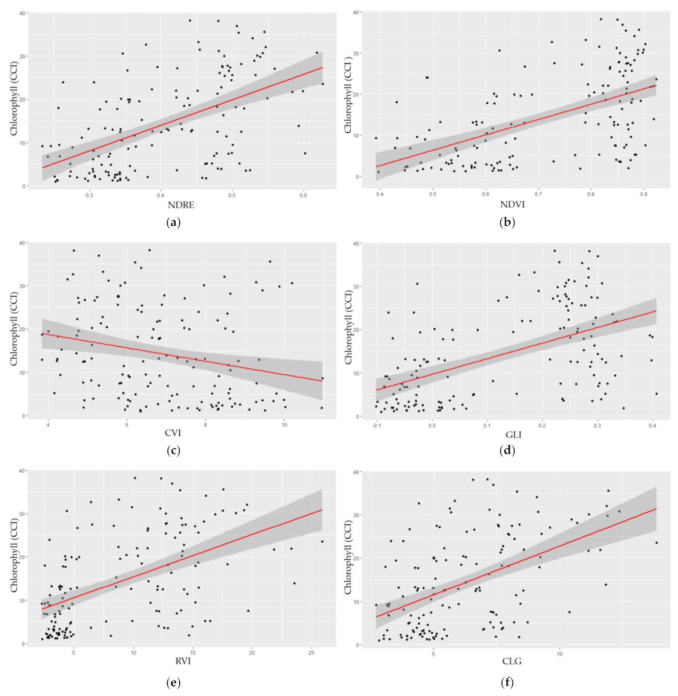
2.1. Chlorophyll Content Measured on the Ground Compared with UAV Derived Vegetation Indices
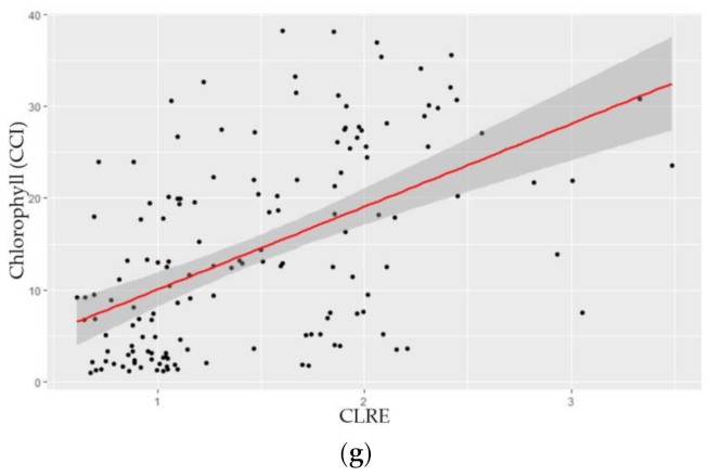
2.2. Comparison between Rust Disease Severity Measured on the Ground and Vegetation Indices
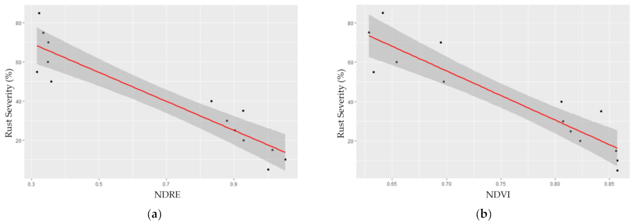
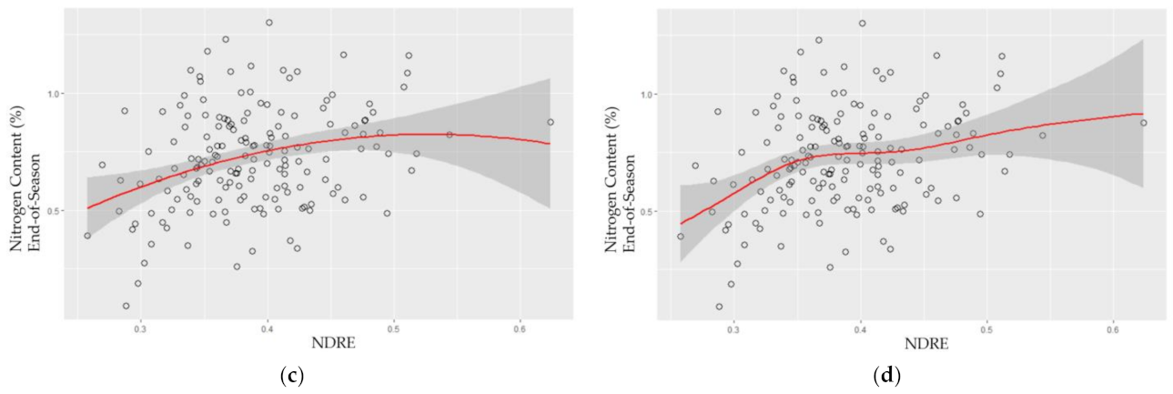
2.3. Nitrogen Content Modeling: Challenges Present in the Results
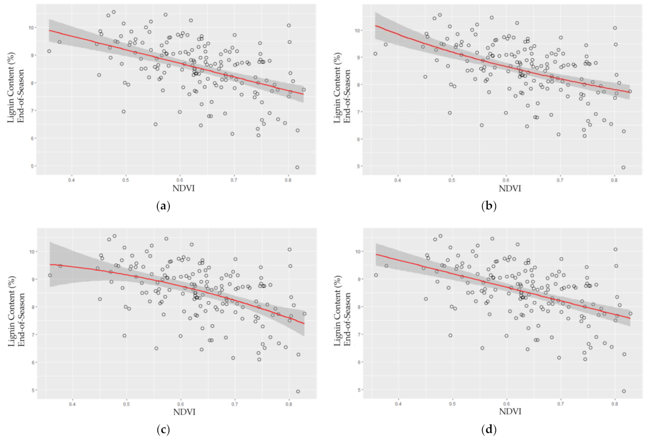
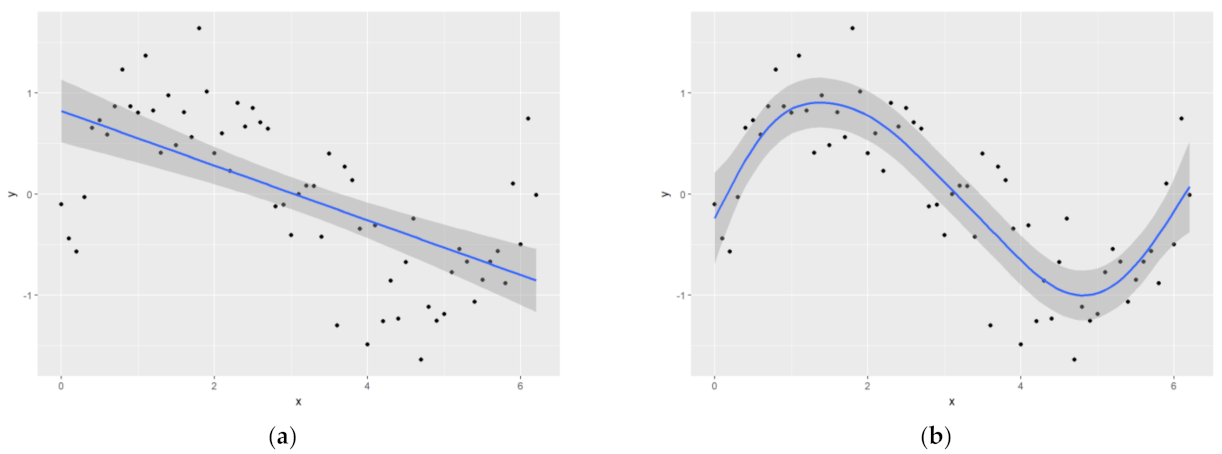
2.4. Polynomial Model Outperformed Other Models for Lignin Content Modeling
3. Discussion
3.1. Model Accuracy
3.2. Vegetation Index Sensitivity and Their Contribution to the Accuracy of the Methodology
3.3. Practical Applications for Agriculture and Forestry
4. Materials and Methods
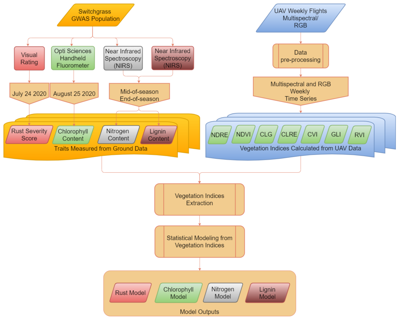
4.1. Data Collection and Processing Overview
4.1.1. Data Collection and Processing Pipeline
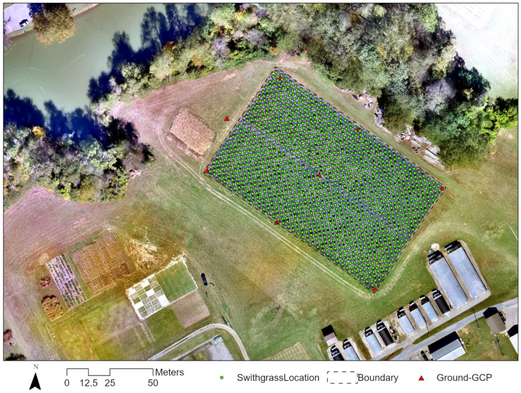
4.1.2. Field Design and Ground Data Collection
4.1.3. UAV Data Collection
4.2. UAV Data Processing
4.2.1. Georeferencing and Mosaicking
4.2.2. Reflectance Calculation
4.3. Data Analysis
4.3.1. Rationale
4.3.2. Remote Sensing Indices
4.3.3. Vegetation Indices Statistics
4.3.4. Model Selection and Evaluation
5. Conclusions
Supplementary Materials
Author Contributions
Funding
Institutional Review Board Statement
Informed Consent Statement
Data Availability Statement
Acknowledgments
Conflicts of Interest
References
- Van Wallendael, A.; Bonnette, J.; Juenger, T.E.; Fritschi, F.B.; Fay, P.A.; Mitchell, R.B.; Lloyd-Reilley, J.; Rouquette, F.M., Jr.; Bergstrom, G.C.; Lowry, D.B. Geographic variation in the genetic basis of resistance to leaf rust between locally adapted ecotypes of the biofuel crop switchgrass (Panicum virgatum). New Phytol. 2020, 227, 1696–1708. [Google Scholar] [CrossRef] [PubMed]
- Uppalapati, S.R.; Serba, D.D.; Ishiga, Y.; Szabo, L.J.; Mittal, S.; Bhandari, H.S.; Bouton, J.H.; Mysore, K.S.; Saha, M.C. Characterization of the rust fungus, Puccinia emaculata, and evaluation of genetic variability for rust resistance in switchgrass populations. BioEnergy Res. 2013, 6, 458–468. [Google Scholar] [CrossRef] [Green Version]
- Loomis, R.S. On the utility of nitrogen in leaves. Proc. Natl. Acad. Sci. USA 1997, 94, 13378–13379. [Google Scholar] [CrossRef] [PubMed] [Green Version]
- Dinh, T.H.; Watanabe, K.; Takaragawa, H.; Nakabaru, M.; Kawamitsu, Y. Photosynthetic response and nitrogen use efficiency of sugarcane under drought stress conditions with different nitrogen application levels. Plant Prod. Sci. 2017, 20, 412–422. [Google Scholar] [CrossRef] [Green Version]
- Owens, V.N.; Viands, D.R.; Mayton, H.S.; Fike, J.H.; Farris, R.; Heaton, E.; Bransby, D.I.; Hong, C.O. Nitrogen use in switchgrass grown for bioenergy across the USA. Biomass Bioenergy 2013, 58, 286–293. [Google Scholar] [CrossRef]
- Lemus, R.; Brummer, C.E.; Burras, L.C.; Moore, K.J.; Barker, M.F.; Molstad, N.E. Effects of nitrogen fertilization on biomass yield and quality in large fields of established switchgrass in southern Iowa, USA. Biomass Bioenergy 2008, 32, 1187–1194. [Google Scholar] [CrossRef] [Green Version]
- Madakadze, I.C.; Stewart, K.A.; Madakadze, R.M.; Peterson, P.R.; Coulman, B.E.; Smith, D.L. Field evaluation of the chlorophyll meter to predict yield and nitrogen concentration of switchgrass. J. Plant Nutr. 1999, 22, 1001–1010. [Google Scholar] [CrossRef]
- Halter, M.; Mitchell, J.; Mann, D.G.J.; Muthukumar, B.; Stewart, C.N., Jr.; Nilsen, E.T. Photosynthetic parameters of switchgrass (Panicum virgatum) under low radiation: Influence of stable overexpression of Miscanthus×giganteus PPDK on responses to light and CO2 under warm and cool growing conditions. New Negat Plant Sci. 2015, 1–2, 23–32. [Google Scholar] [CrossRef] [Green Version]
- Mauromicale, G.; Ierna, A.; Marchese, M. Chlorophyll fluorescence and chlorophyll content in field-grown potato as affected by nitrogen supply, genotype, and plant age. Photosynthetica 2006, 44, 76. [Google Scholar] [CrossRef]
- Yoder, B.J.; Pettigrew-Crosby, R.E. Predicting nitrogen and chlorophyll content and concentrations from reflectance spectra (400–2500 nm) at leaf and canopy scales. Remote Sens. Environ. 1995, 53, 199–211. [Google Scholar] [CrossRef]
- Himmel, M.E.; Bayer, E.A. Lignocellulose conversion to biofuels: Current challenges, global perspectives. Curr. Opin. Biotechnol. 2009, 20, 316–317. [Google Scholar] [CrossRef] [PubMed]
- Ragauskas, A.J.; Beckham, G.T.; Biddy, M.J.; Chandra, R.; Chen, F.; Davis, M.F.; Davison, B.H.; Dixon, R.A.; Gilna, P.; Keller, M.; et al. Lignin valorization: Improving lignin processing in the biorefinery. Science 2014, 344, 1246843. [Google Scholar] [CrossRef] [PubMed]
- Xu, B.; Sathitsuksanoh, N.; Tang, Y.; Udvardi, M.K.; Zhang, J.Y.; Shen, Z.; Balota, M.; Harich, K.; Zhang, P.Y.; Zhao, B. Overexpression of AtLOV1 in switchgrass alters plant architecture, lignin content, and flowering time. PLoS ONE 2012, 7, e47399. [Google Scholar] [CrossRef] [Green Version]
- Potgieter, A.B.; George-Jaeggli, B.; Chapman, S.C.; Laws, K.; Suárez Cadavid, L.A.; Wixted, J.; Watson, J.; Eldridge, M.; Jordan, D.R.; Hammer, G.L. Multi-spectral imaging from an unmanned aerial vehicle enables the assessment of seasonal leaf area dynamics of sorghum breeding lines. Front Plant Sci. 2017, 8, 1532. [Google Scholar] [CrossRef] [PubMed]
- Shafian, S.; Rajan, N.; Schnell, R.; Bagavathiannan, M.; Valasek, J.; Shi, Y.; Olsenholler, J. Unmanned aerial systems-based remote sensing for monitoring sorghum growth and development. PLoS ONE 2018, 13, e0196605. [Google Scholar] [CrossRef] [PubMed] [Green Version]
- Li, J.; Shi, Y.; Veeranampalayam-Sivakumar, A.-N.; Schachtman, D.P. Elucidating sorghum biomass, nitrogen and chlorophyll contents with spectral and morphological traits derived from unmanned aircraft system. Front Plant Sci. 2018, 9, 1406. [Google Scholar] [CrossRef] [PubMed]
- Simic Milas, A.; Romanko, M.; Reil, P.; Abeysinghe, T.; Marambe, A. The importance of leaf area index in mapping chlorophyll content of corn under different agricultural treatments using UAV images. Int. J. Remote Sens. 2018, 39, 5415–5431. [Google Scholar] [CrossRef]
- Kanning, M.; Kühling, I.; Trautz, D.; Jarmer, T. High-resolution UAV-based hyperspectral imagery for LAI and chlorophyll estimations from wheat for yield prediction. Remote Sens. 2018, 10, 2000. [Google Scholar] [CrossRef] [Green Version]
- Shendryk, Y.; Sofonia, J.; Garrard, R.; Rist, Y.; Skocaj, D.; Thorburn, P. Fine-scale prediction of biomass and leaf nitrogen content in sugarcane using UAV LiDAR and multispectral imaging. Int. J. Appl. Earth Obs. Geoinf. 2020, 92, 102177. [Google Scholar] [CrossRef]
- Li, S.; Ding, X.; Kuang, Q.; Ata-UI-Karim, S.T.; Cheng, T.; Liu, X.; Tian, Y.; Zhu, Y.; Cao, W.; Cao, Q. Potential of UAV-based active sensing for monitoring rice leaf nitrogen status. Front Plant Sci. 2018, 9, 1834. [Google Scholar] [CrossRef] [Green Version]
- Lu, N.; Wang, W.; Zhang, Q.; Li, D.; Yao, X.; Tian, Y.; Zhu, Y.; Cao, W.; Baret, F.; Liu, S.; et al. Estimation of nitrogen nutrition status in winter wheat from unmanned aerial vehicle based multi-angular multispectral imagery. Front Plant Sci. 2019, 10, 1601. [Google Scholar] [CrossRef] [PubMed] [Green Version]
- Kefauver, S.C.; Vicente, R.; Vergara-Díaz, O.; Fernandez-Gallego, J.A.; Kerfal, S.; Lopez, A.; Melichar, J.P.E.; Serret Molins, M.D.; Araus, J.L. Comparative UAV and field phenotyping to assess yield and nitrogen use efficiency in hybrid and conventional barley. Front Plant Sci. 2017, 8, 1733. [Google Scholar] [CrossRef] [PubMed]
- Zaman-Allah, M.; Vergara, O.; Araus, J.L.; Tarekegne, A.; Magorokosho, C.; Zarco-Tejada, P.J.; Hornero, A.; Albà, A.H.; Das, B.; Craufurd, P.; et al. Unmanned aerial platform-based multi-spectral imaging for field phenotyping of maize. Plant Methods 2015, 11, 35. [Google Scholar] [CrossRef] [Green Version]
- Schirrmann, M.; Landwehr, N.; Giebel, A.; Garz, A.; Dammer, K.H. Early detection of stripe rust in winter wheat using deep residual neural networks. Front Plant Sci. 2021, 12, 475. [Google Scholar] [CrossRef] [PubMed]
- Li, F.; Piasecki, C.; Millwood, R.J.; Wolfe, B.; Mazarei, M.; Stewart, C.N., Jr. High-Throughput switchgrass phenotyping and biomass modeling by UAV. Front Plant Sci. 2020, 11, 1532. [Google Scholar] [CrossRef] [PubMed]
- Maesano, M.; Khoury, S.; Nakhle, F.; Firrincieli, A.; Gay, A.; Tauro, F.; Harfouche, A. UAV-based LiDAR for high-throughput determination of plant height and above-ground biomass of the bioenergy grass Arundo donax. Remote Sens. 2020, 12, 3464. [Google Scholar] [CrossRef]
- Chen, F.; Dixon, R.A. Lignin modification improves fermentable sugar yields for biofuel production. Nat. Biotechnol. 2007, 25, 759–761. [Google Scholar] [CrossRef]
- Ponnusamy, V.K.; Nguyen, D.D.; Dharmaraja, J.; Shobana, S.; Banu, J.R.; Saratale, R.G.; Chang, S.W.; Kumar, G. A review on lignin structure, pretreatments, fermentation reactions and biorefinery potential. Bioresour. Technol. 2019, 271, 462–472. [Google Scholar] [CrossRef]
- Zhang, Y.; Naebe, M. Lignin: A review on structure, properties, and applications as a light-colored UV absorber. ACS Sustain. Chem. Eng. 2021, 9, 1427–1442. [Google Scholar] [CrossRef]
- Bohnenkamp, D.; Behmann, J.; Mahlein, A.K. In-field detection of yellow rust in wheat on the ground canopy and UAV scale. Remote Sens. 2019, 11, 2495. [Google Scholar] [CrossRef] [Green Version]
- Su, J.Y.; Liu, C.J.; Coombes, M.; Hu, X.P.; Wang, C.H.; Xu, X.M.; Li, Q.D.; Guo, L.; Chen, W.H. Wheat yellow rust monitoring by learning from multispectral UAV aerial imagery. Comput. Electron. Agr. 2018, 155, 157–166. [Google Scholar] [CrossRef]
- Guo, A.T.; Huang, W.J.; Dong, Y.Y.; Ye, H.C.; Ma, H.Q.; Liu, B.; Wu, W.B.; Ren, Y.; Ruan, C.; Geng, Y. Wheat yellow rust detection using UAV-based hyperspectral technology. Remote Sens. 2021, 13, 123. [Google Scholar] [CrossRef]
- Lovell, J.T.; Shakirov, E.V.; Schwartz, S.; Lowry, D.B.; Aspinwall, M.J.; Taylor, S.H.; Bonnette, J.; Palacio-Mejia, J.D.; Hawkes, C.V.; Fay, P.A.; et al. Promises and challenges of eco-physiological genomics in the field: Tests of drought responses in switchgrass. Plant Physiol. 2016, 172, 734–748. [Google Scholar] [CrossRef] [PubMed]
- Humbird, D.; Davis, R.; Tao, L.; Kinchin, C.; Hsu, D.; Aden, A.; Schoen, P.; Lukas, J.; Olthof, B.; Worley, M.; et al. Process Design and Economics for Biochemical Conversion of Lignocellulosic Biomass to Ethanol: Dilute-Acid Pretreatment and Enzymatic Hydrolysis of Corn Stover; National Renewable Energy Lab. (NREL): Golden, CO, USA, 2011; 147p.
- Matsushita, B.; Yang, W.; Chen, J.; Onda, Y.; Qiu, G. Sensitivity of the enhanced vegetation index (EVI) and normalized difference vegetation index (NDVI) to topographic effects: A case study in high-density cypress forest. Sensors 2007, 7, 2636–2651. [Google Scholar] [CrossRef] [Green Version]
- Zhang, K.; Ge, X.; Shen, P.; Li, W.; Liu, X.; Cao, Q.; Zhu, Y.; Cao, W.; Tian, Y. Predicting rice grain yield based on dynamic changes in vegetation indexes during early to mid-growth stages. Remote Sens. 2019, 11, 387. [Google Scholar] [CrossRef] [Green Version]
- Shaver, T.M.; Khosla, R.; Westfall, D.G. Evaluation of two ground-based active crop canopy sensors in maize: Growth stage, row spacing, and sensor movement speed. Soil Sci. Soc. Am. J. 2010, 74, 2101–2108. [Google Scholar] [CrossRef]
- Yu, J.J.; Kim, D.W.; Lee, E.J.; Son, S.W. Determining the optimal number of ground control points for varying study sites through accuracy evaluation of unmanned aerial system-based 3D point clouds and digital surface models. Drones 2020, 4, 49. [Google Scholar] [CrossRef]
- Oniga, V.-E.; Breaban, A.-I.; Statescu, F. Determining the optimum number of ground control points for obtaining high precision results based on UAS images. Proceedings 2018, 2, 352. [Google Scholar] [CrossRef] [Green Version]
- Park, J.W.; Yeom, D.J. Method for establishing ground control points to realize UAV-based precision digital maps of earthwork sites. J. Asian Archit. Build. 2021, 2, 352. [Google Scholar] [CrossRef]
- Ventura, F.; Vignudelli, M.; Letterio, T.; Gentile, S.L.; Anconelli, S. Remote sensing and UAV vegetation index comparison with on-site FAPAR measurement. In Proceedings of the 2019 IEEE International Workshop on Metrology for Agriculture and Forestry (MetroAgriFor), Portici, Italy, 24–26 October 2019; pp. 202–206. [Google Scholar]
- Yang, S.; Bai, J.; Zhao, C.; Lou, H.; Zhang, C.; Guan, Y.; Zhang, Y.; Wang, Z.; Yu, X. The assessment of the changes of biomass and riparian buffer width in the terminal reservoir under the impact of the South-to-North Water Diversion Project in China. Ecol. Indic. 2018, 85, 932–943. [Google Scholar] [CrossRef]
- Possoch, M.; Bieker, S.; Hoffmeister, D.; Bolten, A.; Schellberg, J.; Bareth, G. Multi-temporal crop surface models combined with the RGB vegetation index from UAV-based images for forage monitoring in grassland. Int. Arch. Photogramm. Remote. Sens. Spat. Inf. Sci. Gott. 2016, XLI-B1, 991–998. [Google Scholar] [CrossRef] [Green Version]
- Shen, H.; Fu, C.; Xiao, X.; Ray, T.; Tang, Y.; Wang, Z.; Chen, F. Developmental control of lignification in stems of lowland switchgrass variety Alamo and the effects on saccharification efficiency. BioEnergy Res. 2009, 2, 233–245. [Google Scholar] [CrossRef]
- Jiang, Q.; Fang, S.; Peng, Y.; Gong, Y.; Zhu, R.; Wu, X.; Ma, Y.; Duan, B.; Liu, J. UAV-based biomass estimation for rice-combining spectral, TIN-based structural and meteorological features. Remote Sens. 2019, 11, 890. [Google Scholar] [CrossRef] [Green Version]
- Han, L.; Yang, G.; Dai, H.; Xu, B.; Yang, H.; Feng, H.; Li, Z.; Yang, X. Modeling maize above-ground biomass based on machine learning approaches using UAV remote-sensing data. Plant Methods 2019, 15, 10. [Google Scholar] [CrossRef] [Green Version]
- Yang, M.; Hassan, M.A.; Xu, K.; Zheng, C.; Rasheed, A.; Zhang, Y.; Jin, X.; Xia, X.; Xiao, Y.; He, Z. Assessment of water and nitrogen use efficiencies through UAV-based multispectral phenotyping in winter wheat. Front Plant Sci. 2020, 11. [Google Scholar] [CrossRef]
- Pourazar, H.; Samadzadegan, F.; Javan, F.D. Aerial multispectral imagery for plant disease detection: Radiometric calibration necessity assessment. Eur. J. Remote Sens. 2019, 52, 17–31. [Google Scholar] [CrossRef] [Green Version]
- Brodbeck, C.; Sikora, E.; Delaney, D.; Pate, G.; Johnson, J. Using unmanned aircraft systems for early detection of soybean diseases. Adv. Anim. Biosci. 2017, 8, 802–806. [Google Scholar] [CrossRef]
- Fritschi, F.B.; Ray, J.D. Soybean leaf nitrogen, chlorophyll content, and chlorophyll a/b ratio. Photosynthetica 2007, 45, 92–98. [Google Scholar] [CrossRef]
- Girardin, P.; Tollenaar, M.; Muldoon, J.F. Effect of temporary N starvation on leaf photosynthetic rate and chlorophyll content of maize. Can. J. Plant Sci. 1985, 65, 491–500. [Google Scholar] [CrossRef]
- Guretzky, J.; Biermacher, J.; Cook, B.; Kering, M.; Mosali, J. Switchgrass for forage and bioenergy: Harvest and nitrogen rate effects on biomass yields and nutrient composition. Plant Soil 2010, 339, 69–81. [Google Scholar] [CrossRef] [Green Version]
- Adamec, Z.; Drápela, K. Generalized additive models as an alternative approach to the modeling of the tree height-diameter relationship. J. For. Sci. 2015, 61, 235–243. [Google Scholar] [CrossRef] [Green Version]
- Baxter, H.L.; Mazarei, M.; Fu, C.; Cheng, Q.; Turner, G.B.; Sykes, R.W.; Windham, M.T.; Davis, M.F.; Dixon, R.A.; Wang, Z.-Y.; et al. Time course field analysis of COMT-downregulated switchgrass: Lignification, recalcitrance, and rust susceptibility. BioEnergy Res. 2016, 9, 1087–1100. [Google Scholar] [CrossRef]
- Xie, C.; Yang, C. A review on plant high-throughput phenotyping traits using UAV-based sensors. Comput. Electron. Agr. 2020, 178, 105731. [Google Scholar] [CrossRef]
- Ludovisi, R.; Tauro, F.; Salvati, R.; Khoury, S.; Mugnozza Scarascia, G.; Harfouche, A. UAV-based thermal imaging for high-throughput field phenotyping of black poplar response to drought. Front Plant Sci. 2017, 8, 1681. [Google Scholar] [CrossRef]
- Goggin, F.L.; Lorence, A.; Topp, C.N. Applying high-throughput phenotyping to plant-insect interactions: Picturing more resistant crops. Curr. Opin. Insect. Sci. 2015, 9, 69–76. [Google Scholar] [CrossRef] [PubMed] [Green Version]
- Moreira, F.F.; Oliveira, H.R.; Volenec, J.J.; Rainey, K.M.; Brito, L.F. Integrating high-throughput phenotyping and statistical genomic methods to genetically improve longitudinal traits in crops. Front Plant Sci. 2020, 11, 681. [Google Scholar] [CrossRef] [PubMed]
- Mir, R.R.; Reynolds, M.; Pinto, F.; Khan, M.A.; Bhat, M.A. High-throughput phenotyping for crop improvement in the genomics era. Plant Sci. 2019, 282, 60–72. [Google Scholar] [CrossRef] [PubMed]
- Yang, G.; Liu, J.; Zhao, C.; Li, Z.; Huang, Y.; Yu, H.; Xu, B.; Yang, X.; Zhu, D.; Zhang, X.; et al. Unmanned aerial vehicle remote sensing for field-based crop phenotyping: Current status and perspectives. Front Plant Sci. 2017, 30, 8–1111. [Google Scholar] [CrossRef] [PubMed]
- Chawade, A.; van Ham, J.; Blomquist, H.; Bagge, O.; Alexandersson, E.; Ortiz, R. High-throughput field-phenotyping tools for plant breeding and precision agriculture. Agronomy 2019, 9, 258. [Google Scholar] [CrossRef] [Green Version]
- Sharma, N.; Schneider-Canny, R.; Chekhovskiy, K.; Kwon, S.; Saha, M.C. Opportunities for increased nitrogen use efficiency in wheat for forage use. Plants 2020, 9, 1738. [Google Scholar] [CrossRef]
- Coupel-Ledru, A.; Pallas, B.; Delalande, M.; Boudon, F.; Carrié, E.; Martinez, S.; Regnard, J.-L.; Costes, E. Multi-scale high-throughput phenotyping of apple architectural and functional traits in orchard reveals genotypic variability under contrasted watering regimes. Hortic. Res. 2019, 6, 52. [Google Scholar] [CrossRef] [Green Version]
- Loladze, A.; Rodrigues, F.A.; Toledo, F.; San Vicente, F.; Gérard, B.; Boddupalli, M.P. Application of remote sensing for phenotyping tar spot complex resistance in maize. Front Plant Sci. 2019, 10. [Google Scholar] [CrossRef] [PubMed] [Green Version]
- Hastie, T.J.; Tibshirani, R.J. Generalized Additive Models; Routledge: Abingdon, UK, 2017. [Google Scholar]
- Estes, L.D.; Bradley, B.A.; Beukes, H.; Hole, D.G.; Lau, M.; Oppenheimer, M.G.; Schulze, R.; Tadross, M.A.; Turner, W.R. Comparing mechanistic and empirical model projections of crop suitability and productivity: Implications for ecological forecasting. Glob. Ecol. Biogeogr. 2013, 22, 1007–1018. [Google Scholar] [CrossRef]
- Austin, M.P.; Belbin, L.; Meyers, J.A.; Doherty, M.D.; Luoto, M. Evaluation of statistical models used for predicting plant species distributions: Role of artificial data and theory. Ecol. Modell. 2006, 199, 197–216. [Google Scholar] [CrossRef]
- Yee, T.W.; Mitchell, N.D. Generalized additive models in plant ecology. J. Veg. Sci. 1991, 2, 587–602. [Google Scholar] [CrossRef]
- Tulbure, M.G.; Wimberly, M.C.; Boe, A.; Owens, V.N. Climatic and genetic controls of yields of switchgrass, a model bioenergy species. Agric. Ecosyst. Environ. 2012, 146, 121–129. [Google Scholar] [CrossRef]
- Tinarwo, P.; Zewotir, T.; Nort, D. Modelling the effect of eucalyptus genotypes in the pulping process with generalised additive models and fractional polynomial approaches. Wood Res-Slovak. 2017, 62, 389–404. [Google Scholar]
- Wells, J.M.; Drielak, E.; Surendra, K.C.; Kumar Khanal, S. Hot water pretreatment of lignocellulosic biomass: Modeling the effects of temperature, enzyme and biomass loadings on sugar yield. Bioresour. Technol. 2020, 300, 122593. [Google Scholar] [CrossRef] [PubMed]
- Solanki, H.U.; Bhatpuria, D.; Chauhan, P. Applications of generalized additive model (GAM) to satellite-derived variables and fishery data for prediction of fishery resources distributions in the Arabian Sea. Geocarto. Int. 2017, 32, 30–43. [Google Scholar] [CrossRef]


| VI | NDRE | NDVI | CVI | GLI | RVI | CLG | CLRE |
|---|---|---|---|---|---|---|---|
| Pearson Correlation | 0.5386 | 0.5466 | −0.2433 | 0.5225 | 0.5154 | 0.4975 | 0.5219 |
| R-squared | 0.2852 | 0.2939 | 0.0527 | 0.2681 | 0.2606 | 0.2424 | 0.2674 |
| p-value | 1.664 × 10⁻¹² | 6.659 × 10⁻¹³ | 0.0029 | 9.628 × 10⁻¹² | 2.041 × 10⁻¹¹ | 1.249 × 10⁻¹⁰ | 1.028 × 10⁻¹¹ |
| Linear Regression | Logarithm Transformation | Quadratic Polynomial | Generalized Additive Model (GAM) Model (Nonlinear Effects) | |||||||
|---|---|---|---|---|---|---|---|---|---|---|
| R-Squared | p-Value | R-Squared | p-Value | R-Squared | p-Value | R-Squared | p-Value | RMSE | ||
| Mid-season | NDVI | 0.0020 | 0.3735 | 0.0025 | 0.3246 | 0.0083 | 0.3576 | 0.0187 | 0.1810 | 0.2466 |
| NDRE | 0.0038 | 0.2284 | 0.0027 | 0.3085 | 0.0130 | 0.1684 | 0.0007 | 0.0281 * | 0.2483 | |
| End-of-season | NDVI | 0.013 | 0.0797 | 0.0111 | 0.0131 * | 0.0299 | 0.0008 * | 0.0458 | 0.0231 * | 0.2130 |
| NDRE | 0.0512 | 2.12 × 10⁻⁷ * | 0.0190 | 0.0011 * | 0.0306 | 0.0007 * | 0.0521 | 0.0110 * | 0.2117 | |
| Linear Regression | Logarithm Transformation | Quadratic Polynomial | Generalized Additive Model (GAM) Model (Linear and Nonlinear Effects) | ||||||||
|---|---|---|---|---|---|---|---|---|---|---|---|
| R-Squared | p-Value | R-Squared | p-Value | R-Squared | p-Value | R-Squared | RMSE | p-Value Linear Effect | p-Value Nonlinear Effect | ||
| Mid-season | NDVI | 0.0319 | 0.0002 * | 0.0306 | 0.0003 * | 0.0368 | 0.0015 * | 0.0092 | 0.8089 | 0.0001 * | 0.0002 * |
| NDRE | 0.0433 | 2.00 × 10⁻⁵ * | 0.0421 | 2.65 × 10⁻⁵ * | 0.0587 | 1.73 × 10⁻⁵ * | 0.0223 | 0.7988 | 1.8 × 10⁻⁵ * | 0.0558 | |
| End-of-season | NDVI | 0.2725 | 2.2 × 10⁻¹⁶ * | 0.2686 | 2.2 × 10⁻¹⁶ * | 0.2727 | 2.2 × 10⁻¹⁶ * | 0.2329 | 0.8730 | 2.2 × 10⁻¹⁶ * | 0.9414 |
| NDRE | 0.1839 | 2.2 × 10⁻¹ 6* | 0.1888 | 2.2 × 10⁻¹⁶ * | 0.1905 | 2.2 × 10⁻¹⁶ * | 0.1621 | 0.9122 | 2.2 × 10⁻¹⁶ * | 0.1502 | |
| Dates of Ground-Based Data | Dates of UAV-Based Data | |
|---|---|---|
| Chlorophyll | 25 August 2020 | 26 August 2020 |
| Rust Disease | 24 July 2020 | 29 July 2020 |
| Nitrogen and Lignin | 4 August 2020 | 29 July 2020 |
| 10 November 2020 | 5 November 2020 |
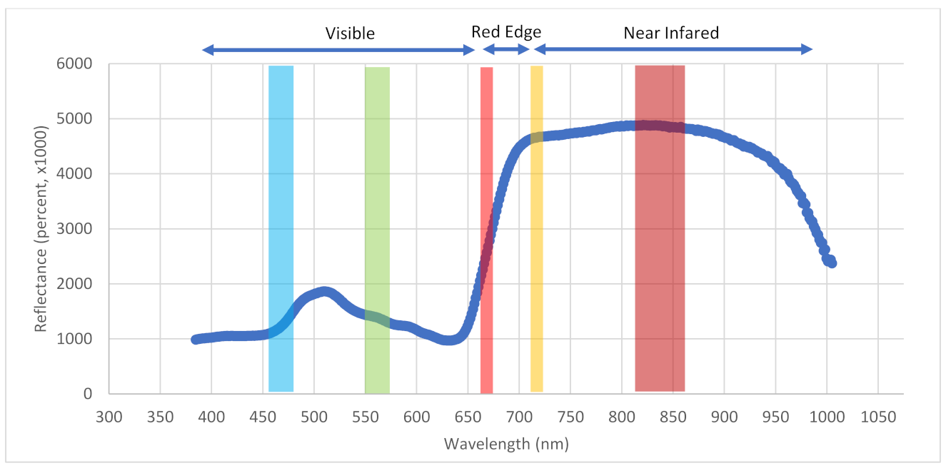
| Band Number | Band Name | Wavelength (nm) |
|---|---|---|
| 1 | Blue | 465–485 |
| 2 | Green | 550–570 |
| 3 | Red | 663–673 |
| 4 | Near Infrared | 820–860 |
| 5 | Red Edge | 712–722 |
| Vegetation Index | Definition | Commonly Used for |
|---|---|---|
| NDRE | normalized difference red edge | chlorophyll, nitrogen, disease |
| NDVI | normalized vegetation index | vegetation cover, chlorophyll, disease |
| CLG | chlorophyll index green | chlorophyll |
| CLRE | chlorophyll index red edge | chlorophyll |
| CVI | chlorophyll vegetation index | chlorophyll |
| GLI | green leaf index | greenness |
| RVI | ratio vegetation index | leaf area index, biomass |
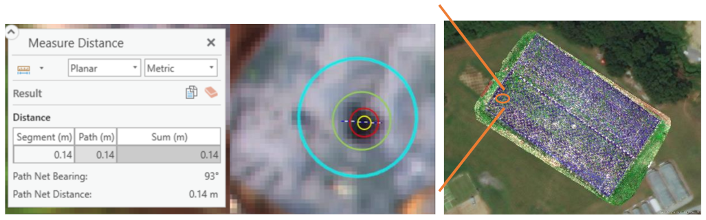
| Buffer Zone Size (Diameter) | Sample Size (Pixels) | Impact |
|---|---|---|
| 40 cm | 480–640 | Oversampled, soil included |
| 20 cm | 120–160 | Oversampled, soil included |
| 10 cm | 30–40 | Sufficient samples representing the proper area size of the switchgrass canopy. |
| 5 cm | 7–10 | Insufficient samples due to under-sampled buffer zone size |
Publisher’s Note: MDPI stays neutral with regard to jurisdictional claims in published maps and institutional affiliations. |
© 2021 by the authors. Licensee MDPI, Basel, Switzerland. This article is an open access article distributed under the terms and conditions of the Creative Commons Attribution (CC BY) license (https://creativecommons.org/licenses/by/4.0/).
Share and Cite
Xu, Y.; Shrestha, V.; Piasecki, C.; Wolfe, B.; Hamilton, L.; Millwood, R.J.; Mazarei, M.; Stewart, C.N. Sustainability Trait Modeling of Field-Grown Switchgrass (Panicum virgatum) Using UAV-Based Imagery. Plants 2021, 10, 2726. https://doi.org/10.3390/plants10122726
Xu Y, Shrestha V, Piasecki C, Wolfe B, Hamilton L, Millwood RJ, Mazarei M, Stewart CN. Sustainability Trait Modeling of Field-Grown Switchgrass (Panicum virgatum) Using UAV-Based Imagery. Plants. 2021; 10(12):2726. https://doi.org/10.3390/plants10122726
Chicago/Turabian StyleXu, Yaping, Vivek Shrestha, Cristiano Piasecki, Benjamin Wolfe, Lance Hamilton, Reginald J. Millwood, Mitra Mazarei, and Charles Neal Stewart. 2021. "Sustainability Trait Modeling of Field-Grown Switchgrass (Panicum virgatum) Using UAV-Based Imagery" Plants 10, no. 12: 2726. https://doi.org/10.3390/plants10122726