
Seasonal Dynamics of Photochemical Performance of PS II of Terrestrial Mosses from Different Elevations


Abstract
:1. Introduction
2. Results
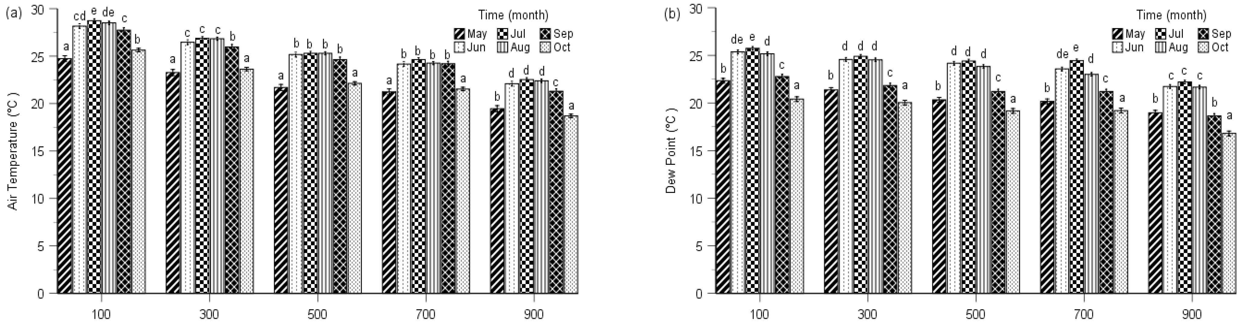
2.1. Seasonal Changes of Environmental Factors
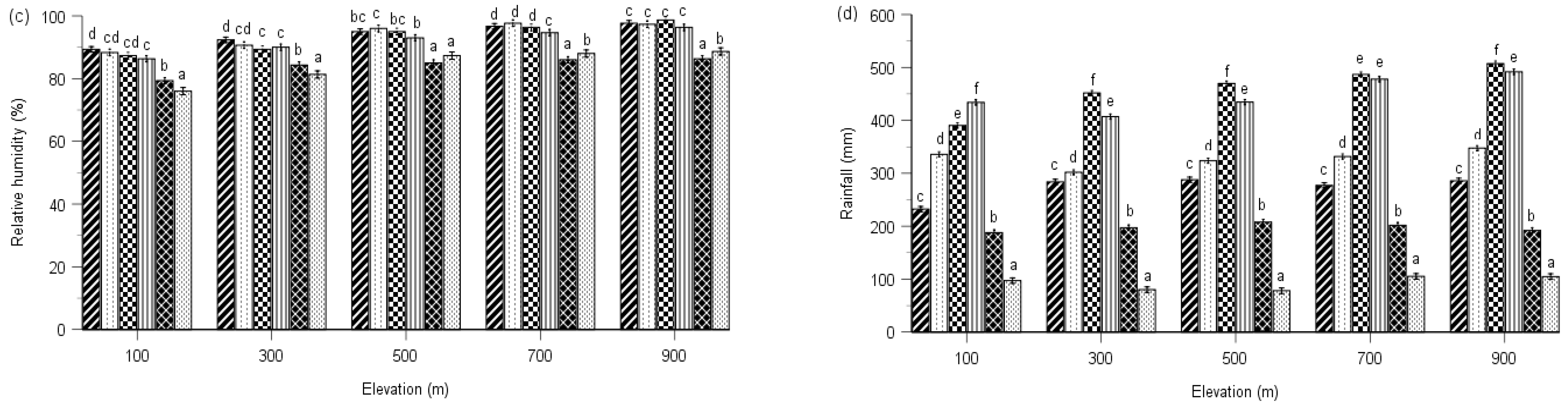
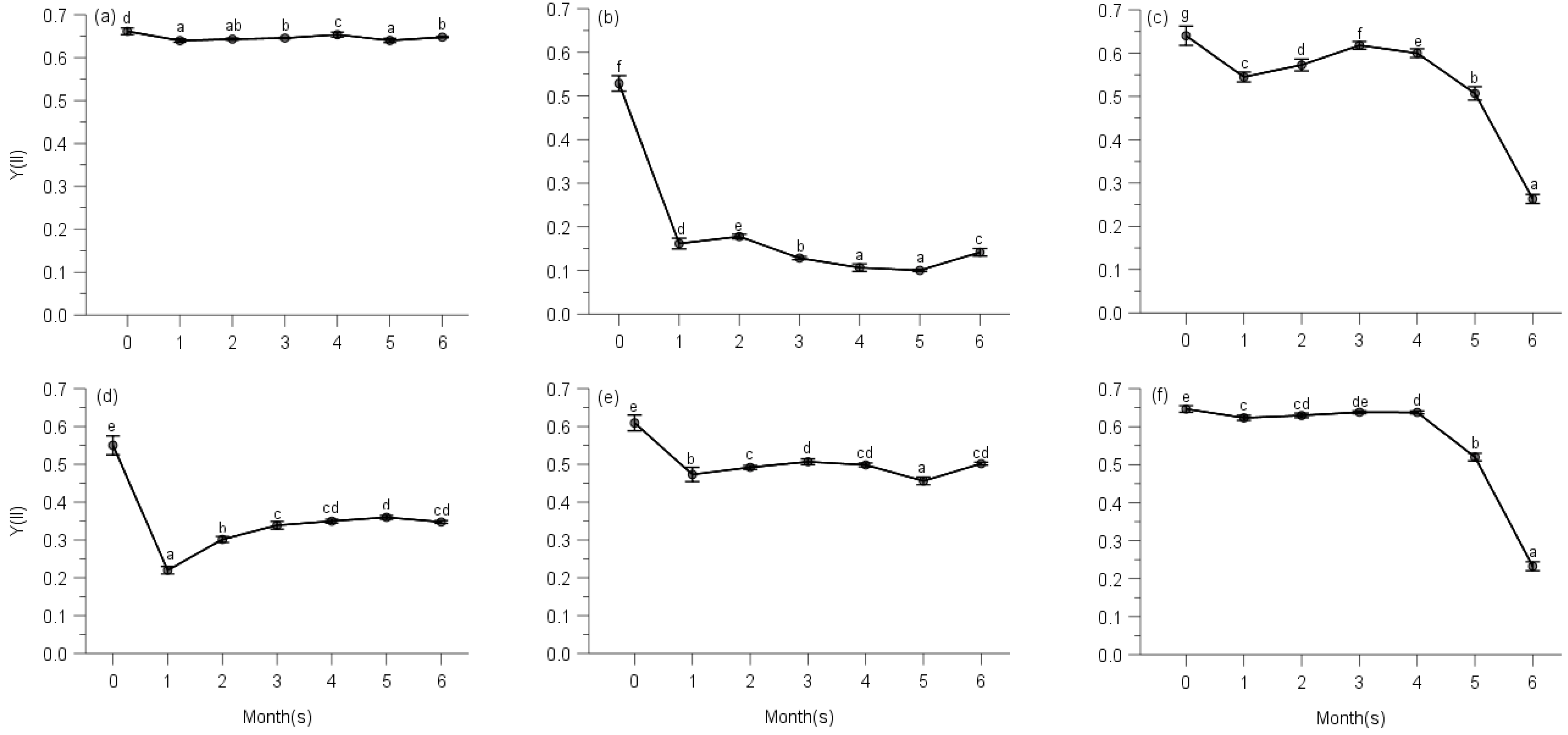
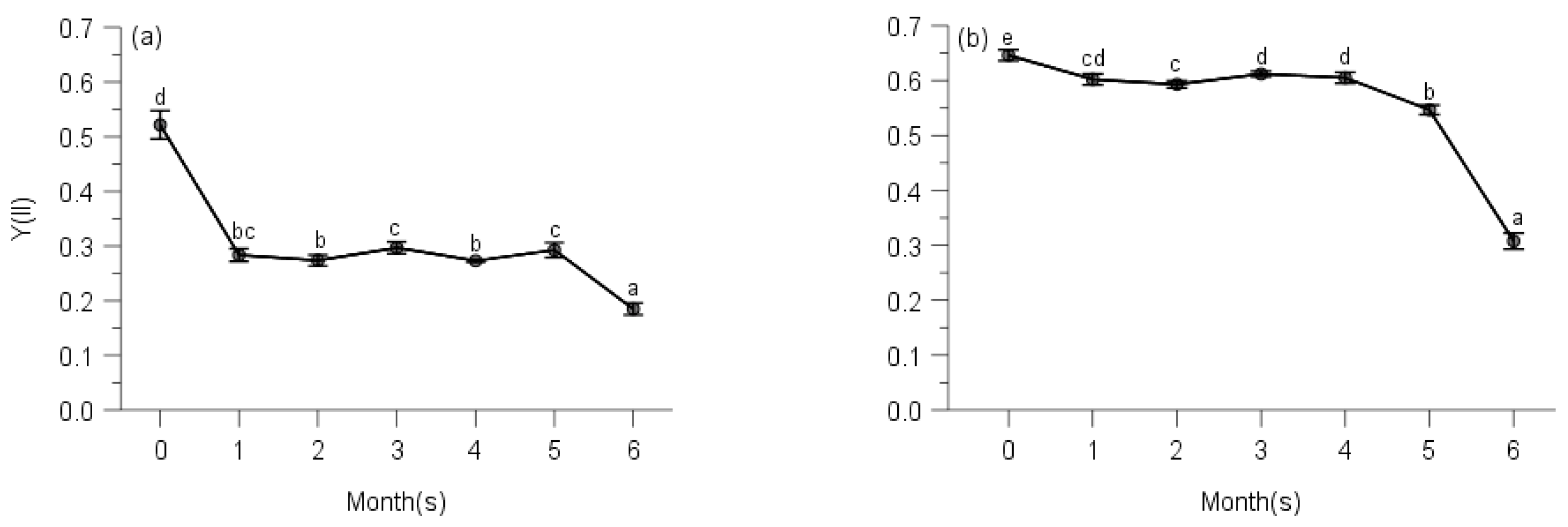
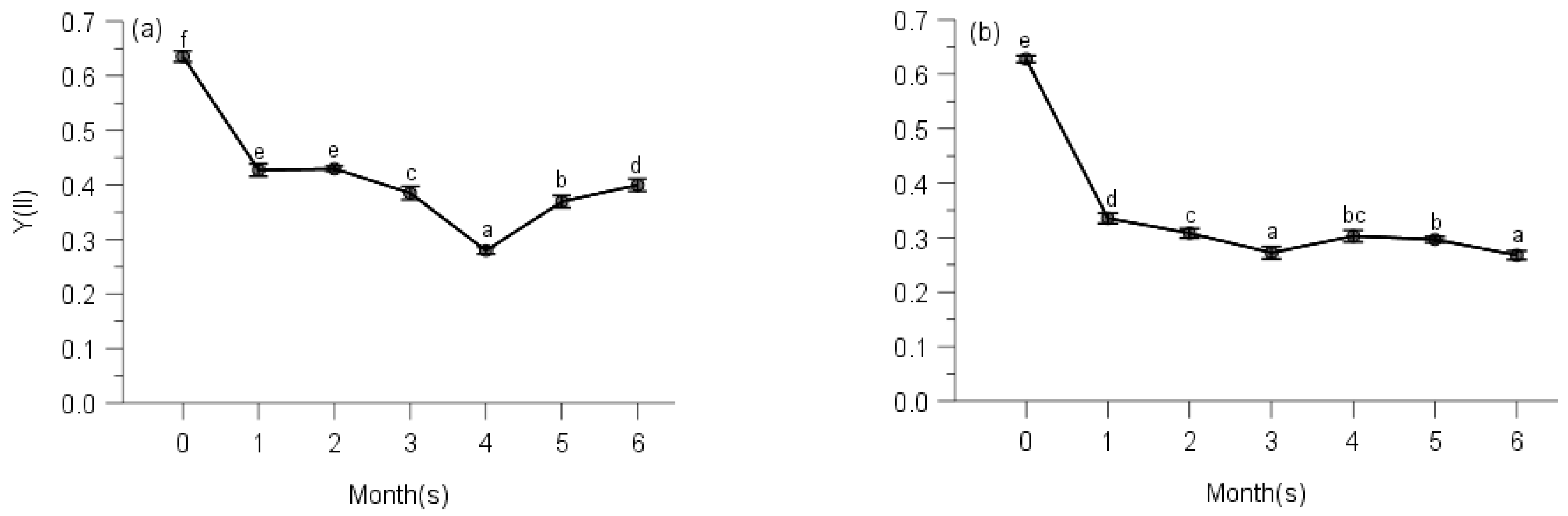
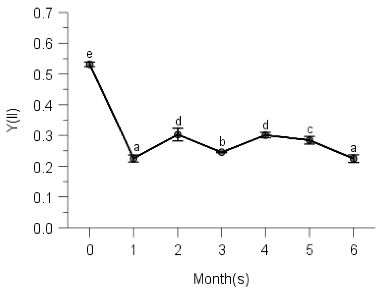
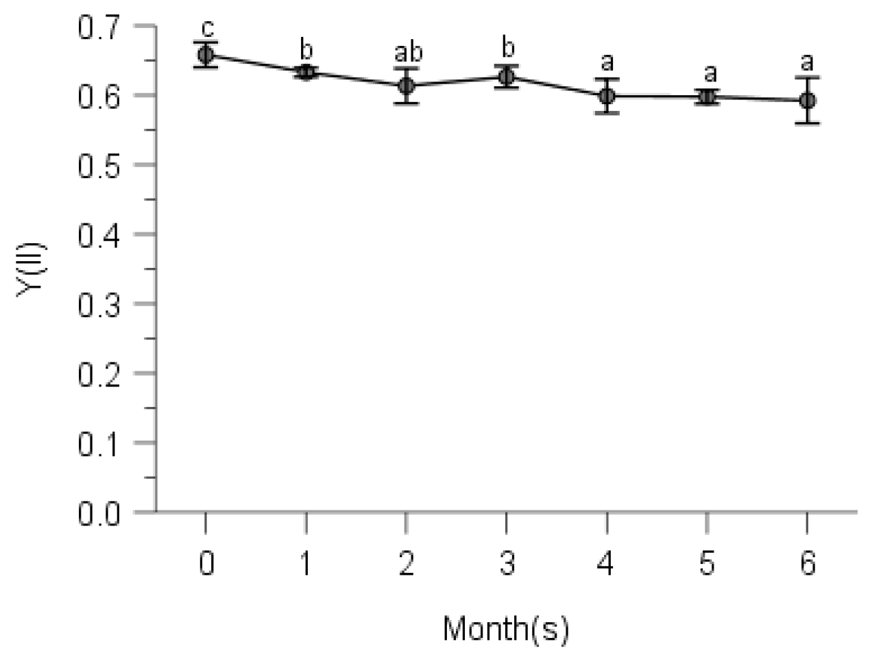
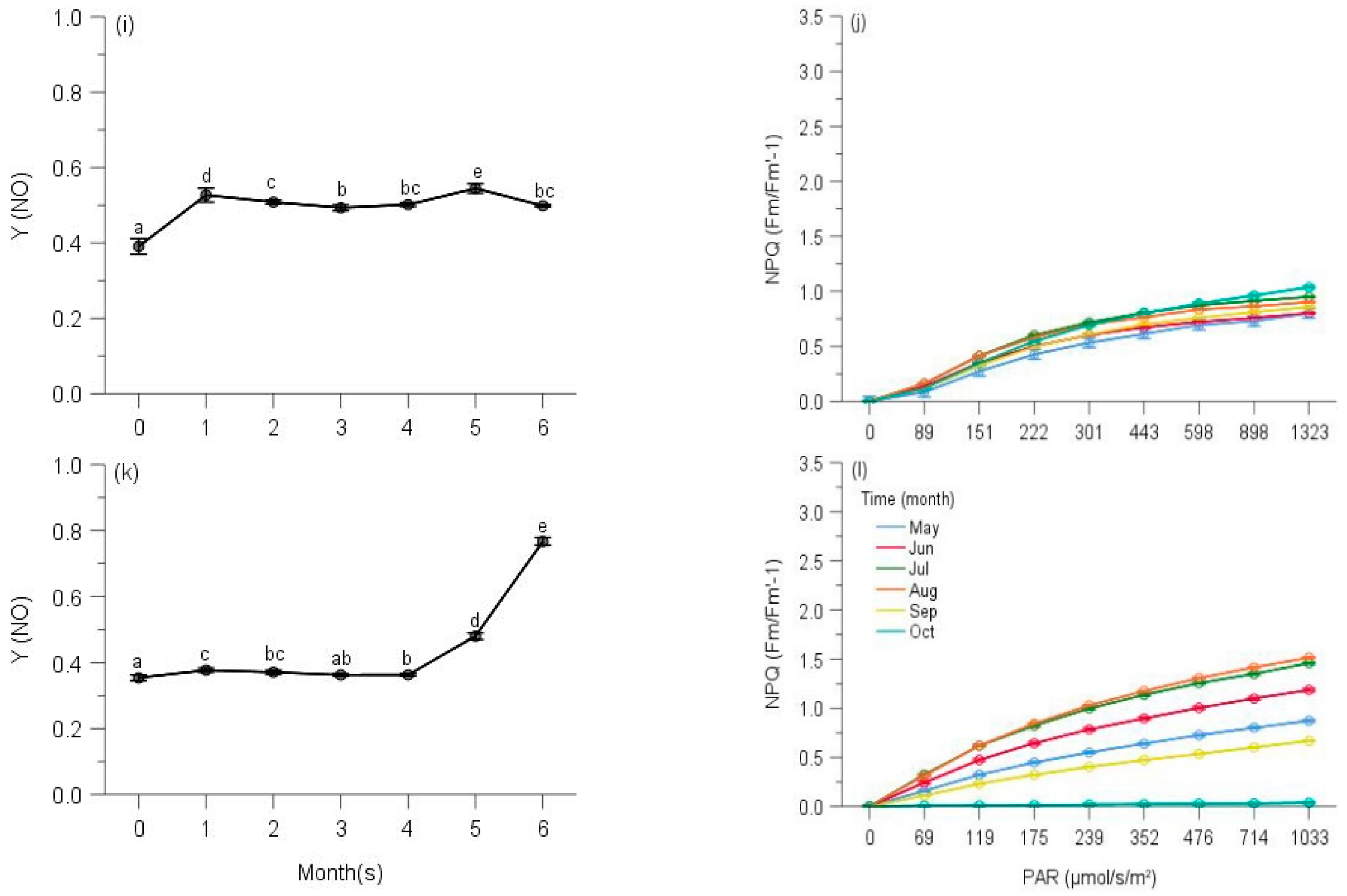
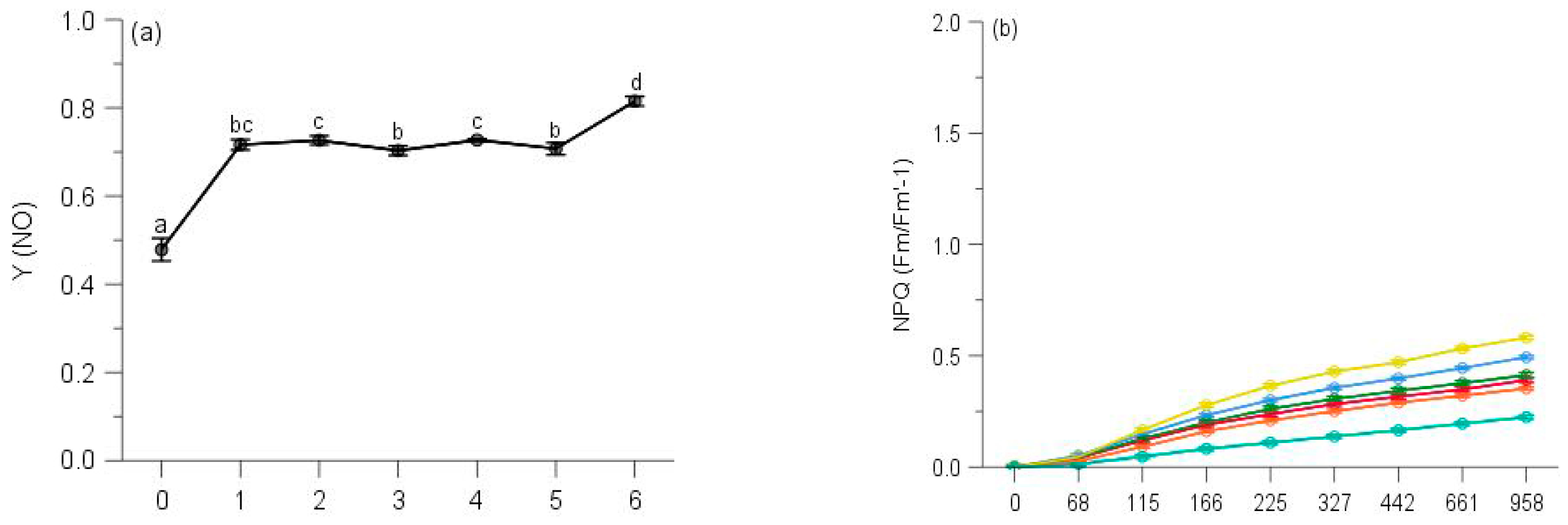
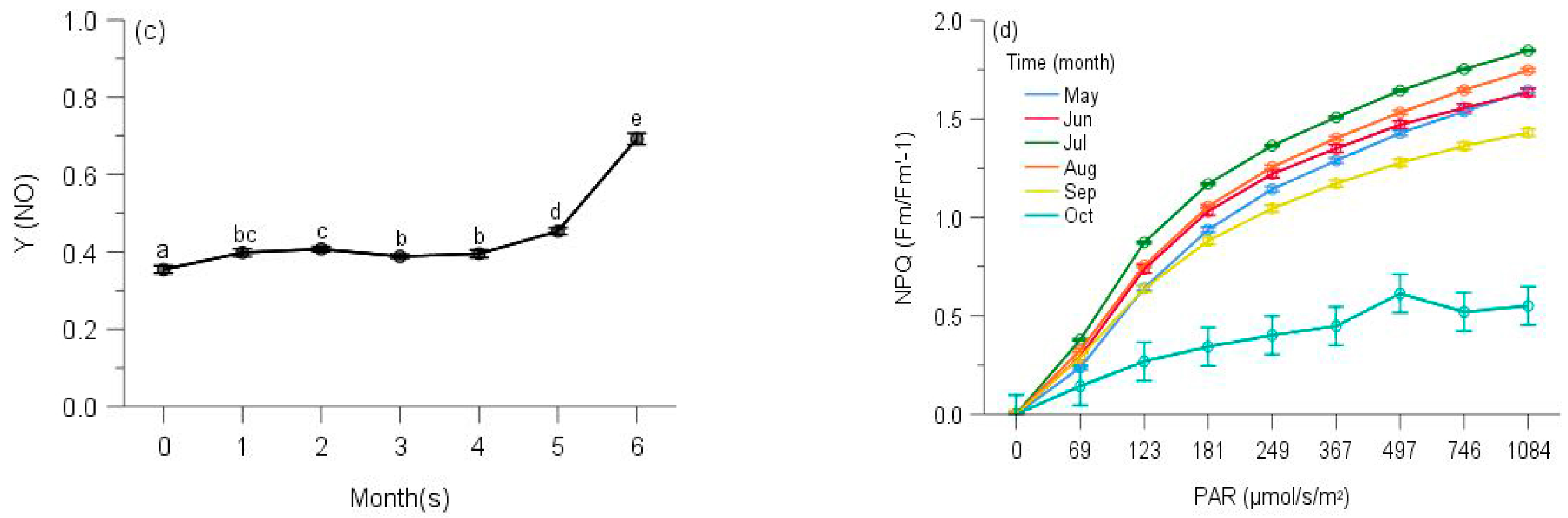
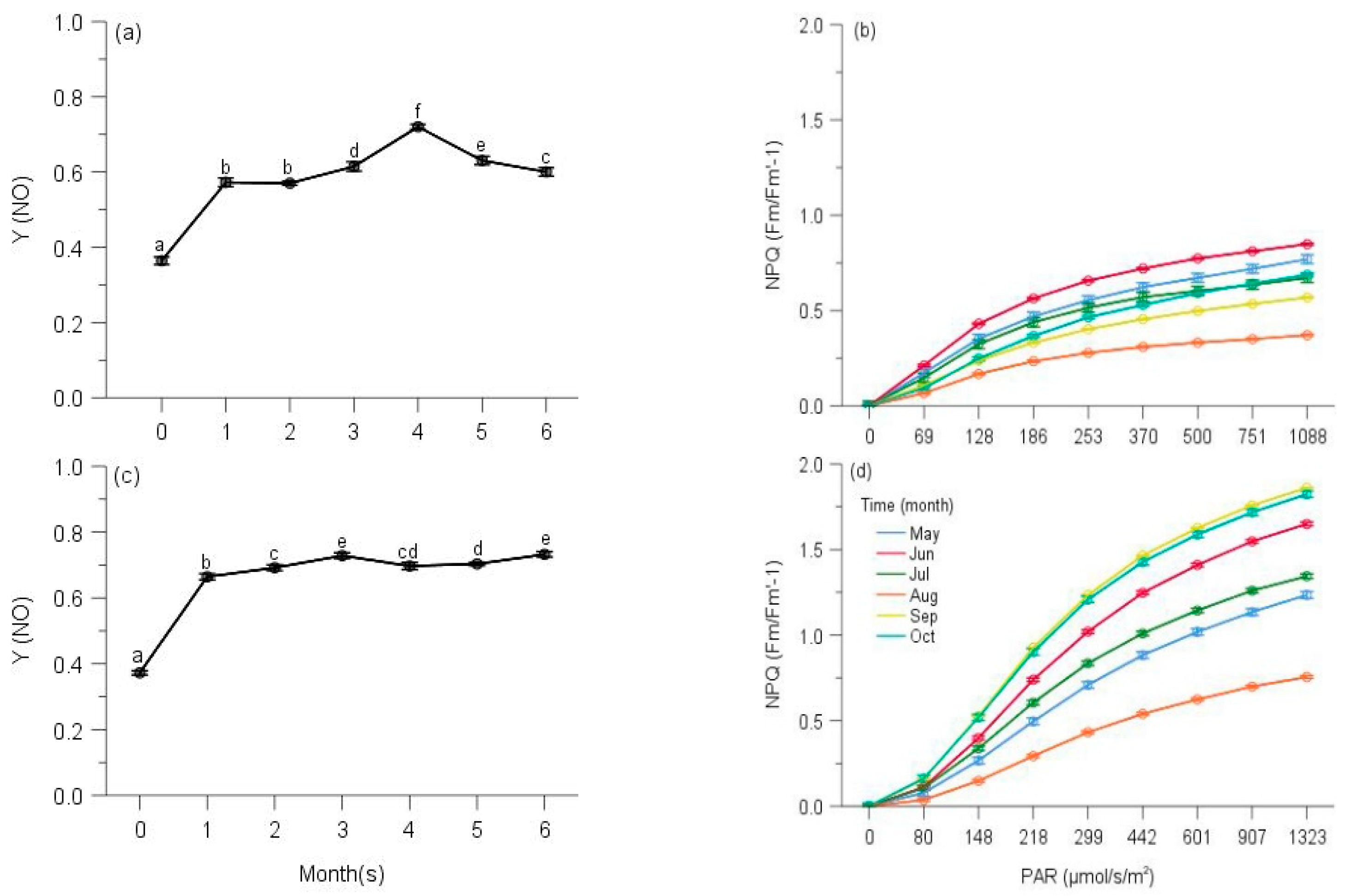
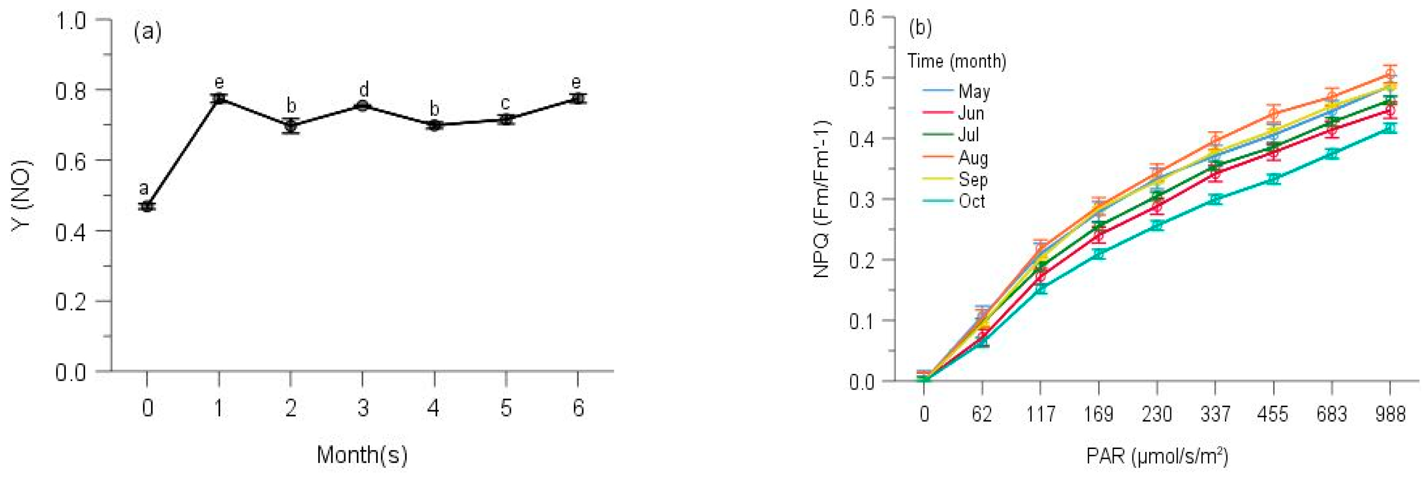
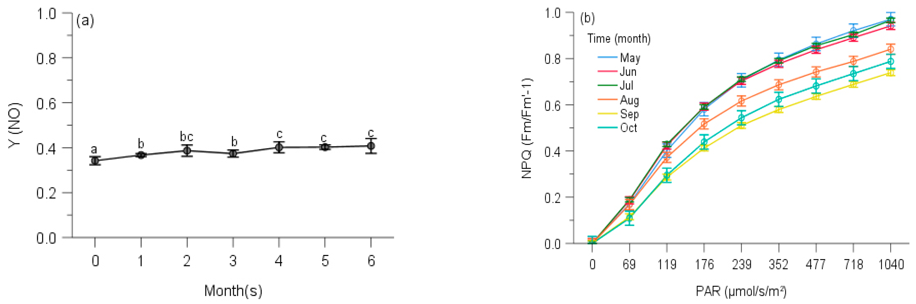
2.2. PSII Photochemistry
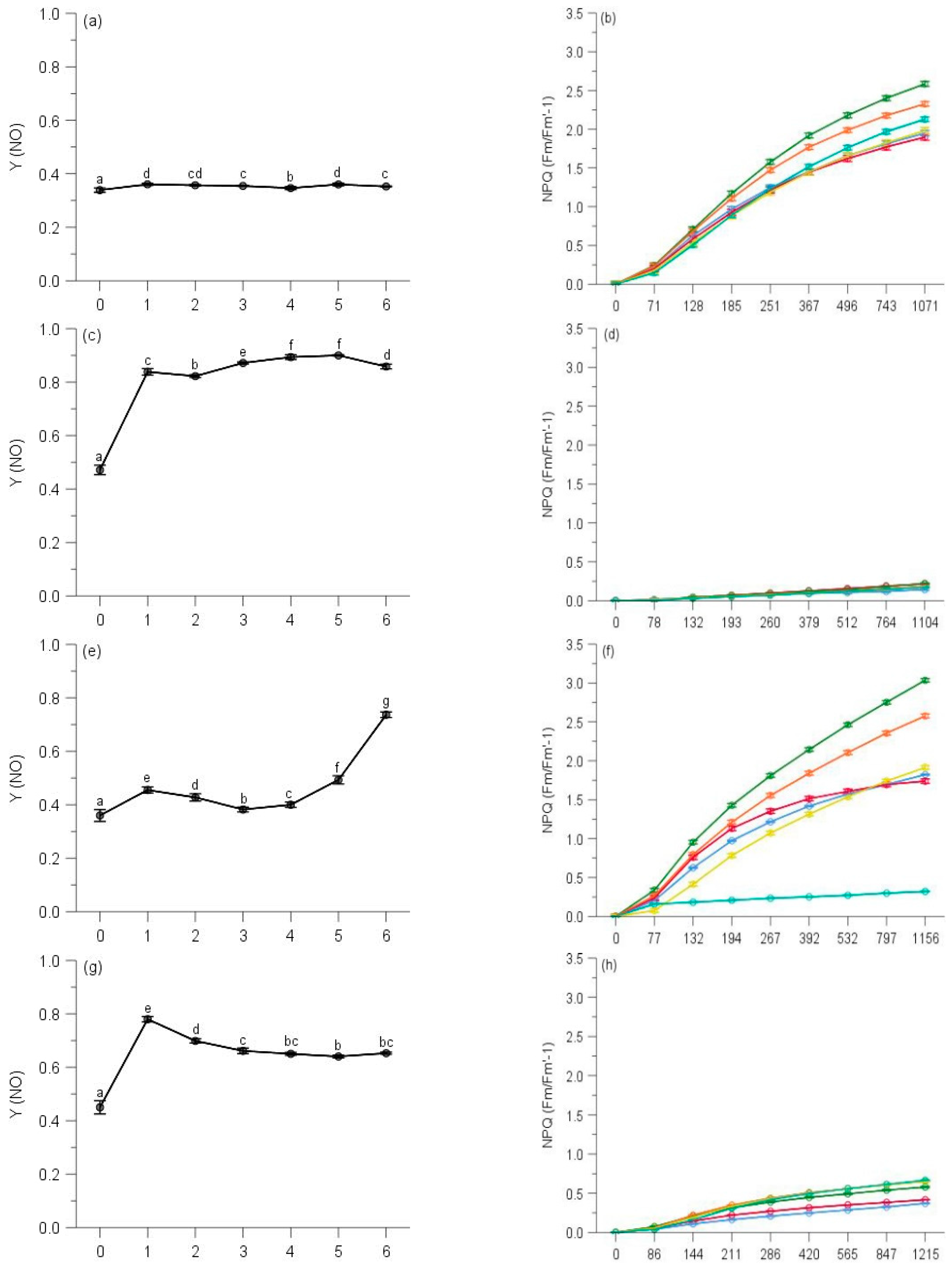
2.3. Regulated and Non-Regulated Energy Dissipation
3. Discussion
4. Materials and Methods
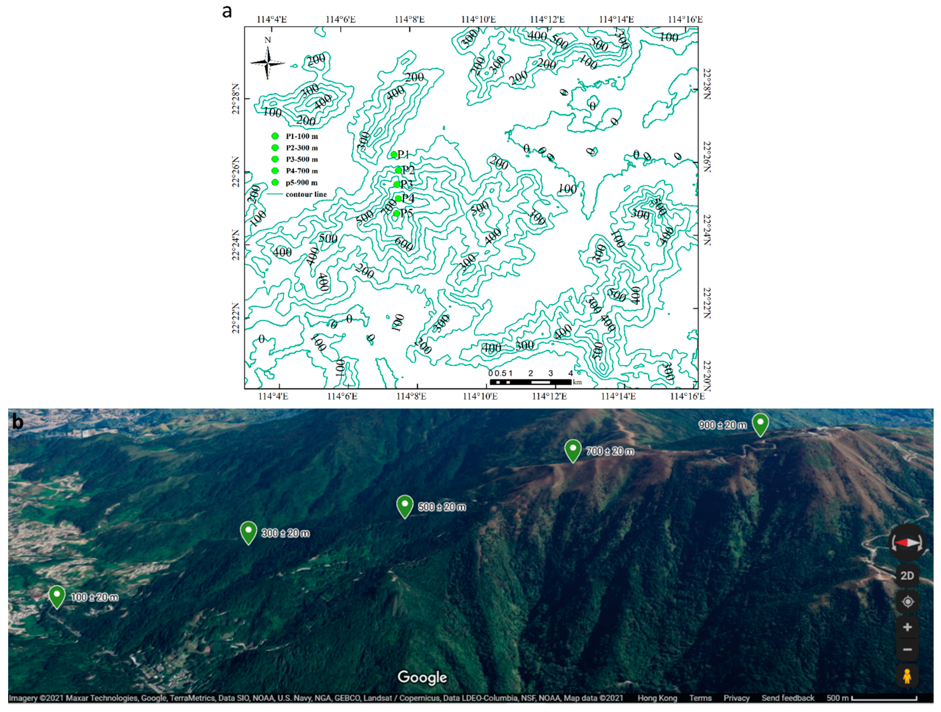
4.1. Study Area
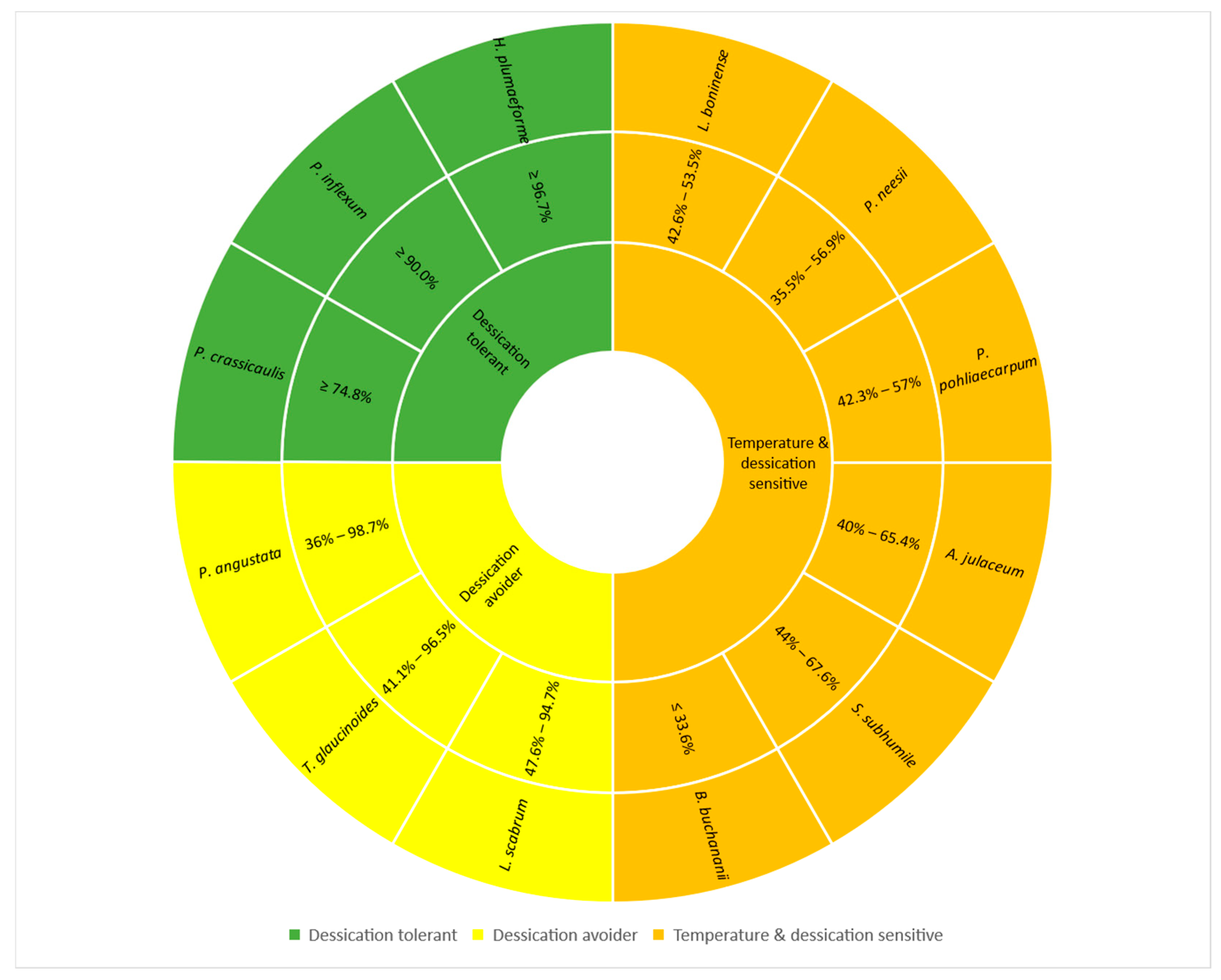
4.2. Study Species
4.3. Chlorophyll Fluorescence Measurements
4.4. Environmental and Climatic Factors
4.5. Statistical Analysis
5. Conclusions
Author Contributions
Funding
Data Availability Statement
Conflicts of Interest
Appendix A

| Altitude (m) | Measure | df | F | p |
|---|---|---|---|---|
| 900 | Air temperature | 5 | 252.944 | <0.001 |
| Dew point | 5 | 460.868 | <0.001 | |
| Relative humidity | 5 | 122.333 | <0.001 | |
| Rainfall | 5 | 5919.829 | <0.001 | |
| 700 | Air temperature | 5 | 158.187 | <0.001 |
| Dew point | 5 | 147.530 | <0.001 | |
| Relative humidity | 5 | 254.240 | <0.001 | |
| Rainfall | 5 | 3020.540 | <0.001 | |
| 500 | Air temperature | 5 | 150.962 | <0.001 |
| Dew point | 5 | 310.839 | <0.001 | |
| Relative humidity | 5 | 71.350 | <0.001 | |
| Rainfall | 5 | 3661.869 | <0.001 | |
| 300 | Air temperature | 5 | 219.498 | <0.001 |
| Dew point | 5 | 670.124 | <0.001 | |
| Relative humidity | 5 | 75.954 | <0.001 | |
| Rainfall | 5 | 6.106 | <0.01 | |
| 100 | Air temperature | 5 | 220.179 | <0.001 |
| Dew point | 5 | 930.688 | <0.001 | |
| Relative humidity | 5 | 100.763 | <0.001 | |
| Rainfall | 5 | 4624.528 | <0.001 |
Appendix B
| Altitude (m) | Species Name | df | F | p |
|---|---|---|---|---|
| 900 | Hypnum plumaeforme | 6 | 54.765 | <0.001 |
| Brachythecium buchananii | 6 | 4476.718 | <0.001 | |
| Thuidium glaucinoides | 6 | 1585.716 | <0.001 | |
| Anomobryum julaceum | 6 | 1345.491 | <0.001 | |
| Pterobryopsis crassicaulis | 6 | 312.981 | <0.001 | |
| Pseudosymblepharis angustata | 6 | 6982.168 | <0.001 | |
| 700 | Pogonatum neesii | 6 | 1035.626 | <0.001 |
| Leucobryum scabrum | 6 | 2610.740 | <0.001 | |
| 500 | Sematophyllum subhumile | 6 | 2165.445 | <0.001 |
| Leucobryum boninense | 6 | 3889.871 | <0.001 | |
| 300 | Pseudotaxiphyllum pohliaecarpum | 6 | 1463.714 | <0.001 |
| 100 | Pogonatum inflexum | 6 | 23.889 | <0.001 |
Appendix C
| Altitude (m) | Species Name | df | F | p |
|---|---|---|---|---|
| 900 | Hypnum plumaeforme | |||
| Y(NO) | 6 | 54.765 | <0.001 | |
| NPQ | 5 | 683.014 | <0.001 | |
| Brachythecium buchananii | ||||
| Y(NO) | 6 | 4476.718 | <0.001 | |
| NPQ | 5 | 101.123 | <0.001 | |
| Thuidium glaucinoides | ||||
| Y(NO) | 6 | 1585.716 | <0.001 | |
| NPQ | 5 | 22,168.897 | <0.001 | |
| Anomobryum julaceum | ||||
| Y(NO) | 6 | 1345.491 | <0.001 | |
| NPQ | 5 | 8337.127 | <0.001 | |
| Pterobryopsis crassicaulis | ||||
| Y(NO) | 6 | 299.129 | <0.001 | |
| NPQ | 5 | 370.082 | <0.001 | |
| Pseudosymblepharis angustata | ||||
| Y(NO) | 6 | 6982.168 | <0.001 | |
| NPQ | 5 | 47,520.709 | <0.001 | |
| 700 | Pogonatum neesii | |||
| Y(NO) | 6 | 1035.626 | <0.001 | |
| NPQ | 5 | 2354.901 | <0.001 | |
| Leucobryum scabrum | ||||
| Y(NO) | 6 | 2610.740 | <0.001 | |
| NPQ | 5 | 1870.289 | <0.001 | |
| 500 | Sematophyllum subhumile | |||
| Y(NO) | 6 | 2165.445 | <0.001 | |
| NPQ | 5 | 2333.928 | <0.001 | |
| Leucobryum boninense | ||||
| Y(NO) | 6 | 4288.060 | <0.001 | |
| NPQ | 5 | 15,013.965 | <0.001 | |
| 300 | Pseudotaxiphyllum pohliaecarpum | |||
| Y(NO) | 6 | 1463.714 | <0.001 | |
| NPQ | 5 | 212.636 | <0.001 | |
| 100 | Pogonatum inflexum | |||
| Y(NO) | 6 | 23.889 | <0.001 | |
| NPQ | 5 | 446.211 | <0.001 |
References
- Kalaji, M.H.; Carpentier, R.; Allakhverdiev, S.I.; Bosa, K. Fluorescence parameters as early indicators of light stress in barley. J. Photochem. Photobiol. B Biol. 2012, 112, 1–6. [Google Scholar] [CrossRef] [PubMed]
- Li, Z.; Wakao, S.; Fischer, B.B.; Niyogi, K.K. Sensing and responding to excess light. Ann. Rev. Plant Biol. 2009, 60, 239–260. [Google Scholar] [CrossRef] [PubMed]
- Pinnola, A.; Bassi, R. Molecular mechanisms involved in plant photoprotection. Biochem. Soc. Trans. 2018, 46, 467–482. [Google Scholar] [CrossRef] [PubMed]
- Ruban, A.V. Nonphotochemical chlorophyll fluorescence quenching: Mechanism and effectiveness in protecting plants from photodamage. Plant Physiol. 2016, 170, 1903–1916. [Google Scholar] [CrossRef] [Green Version]
- Hedges, S.B. The origin and evolution of model organisms. Nat. Rev. Genet. 2002, 3, 838–849. [Google Scholar] [CrossRef]
- Karol, K.G.; Arumuganathan, K.; Boore, J.L.; Duffy, A.M.; Everett, K.D.E.; Hall, J.D.; Hansen, S.K.; Kuehl, J.V.; Mandoli, D.F.; Mishler, B.D.; et al. Complete plastome sequences of Equisetum arvense and Isoetes flaccida: Implications for phylogeny and plastid genome evolution of early land plant lineages. BMC Evol. Biol. 2010, 10, 321. [Google Scholar] [CrossRef] [Green Version]
- Konrat, M.; Shaw, A.J.; Renzaglia, K.S. A special issue of Phytotaxa dedicated to Bryophytes: The closest living relatives of early land plants. Phytotaxa 2010, 9, 5–10. [Google Scholar] [CrossRef]
- Hanson, D.T.; Rice, S.K. What can we learn from bryophyte photosynthesis? In Photosynthesis in Bryophytes and Early Land Plants, Advances in Photosynthesis and Respiration; Hanson, D.T., Rice, S.K., Eds.; Springer: Dordrecht, The Netherlands, 2014; Volume 37, pp. 1–8. [Google Scholar]
- He, X.L.; He, K.S.; Hyvönen, J. Will bryophytes survive in a warming world? Perspect. Plant Ecol. Evol. Syst. 2016, 19, 49–60. [Google Scholar] [CrossRef]
- Halbritter, A.H.; De Boeck, H.J.; Eycott, A.E.; Reinsch, S.; Robinson, D.A.; Vicca, S.; Berauer, B.; Christiansen, C.T.; Estiarte, M.; Grünzweig, J.M.; et al. The handbook for standardized field and laboratory measurements in terrestrial climate change experiments and observational studies (ClimEx). Methods Ecol. Evol. 2020, 11, 22–37. [Google Scholar] [CrossRef] [Green Version]
- Logan, B.A.; Adams III, W.W.; Demmig-Adams, B. Avoiding common pitfalls of chlorophyll fluorescence analysis under field conditions. Funct. Plant Biol. 2007, 34, 853–859. [Google Scholar] [CrossRef] [PubMed]
- Durako, M.J. Using PAM fluorometry for landscape-level assessment of Thalassia testudinum: Can diurnal variation in photochemical efficiency be used as an ecoindicator of seagrass health? Ecol. Indic. 2012, 18, 243–251. [Google Scholar] [CrossRef]
- Brooks, M.D.; Niyogi, K.K. Use of a pulse-amplitude modulated chlorophyll fluorometer to study the efficiency of photosynthesis in Arabidopsis plants. Methods Mol. Biol. 2011, 775, 299–310. [Google Scholar] [CrossRef]
- Campbell, S.; Miller, C.; Steven, A.; Stephens, A. Photosynthetic responses of two temperate seagrasses across a water quality gradient using chlorophyll fluorescence. J. Exp. Mar. Biol. Ecol. 2003, 291, 57–78. [Google Scholar] [CrossRef]
- Adams III, W.W.; Demmig-Adams, B. Chlorophyll fluorescence as a tool to monitor plant response to the environment. In Chlorophyll a Fluorescence. Advances in Photosynthesis and Respiration; Papageorgiou, G.C., Govindjee, Eds.; Springer: Dordrecht, The Netherlands, 2004; Volume 19, pp. 583–604. [Google Scholar] [CrossRef]
- Schreiber, U.; Schliwa, U.; Bilger, W. Continuous recording of photochemical and non-photochemical chlorophyll fluorescence quenching with a new type of modulation fluorometer. Photosyn. Res. 1986, 10, 51–62. [Google Scholar] [CrossRef] [PubMed]
- Ralph, P.J.; Schreiber, U.; Gademann, R.; Kühl, M.; Larkum, A.W.D. Coral photobiology studied with a new imaging pulse amplitude modulated fluorometer. J. Phycol. 2005, 41, 335–342. [Google Scholar] [CrossRef]
- Ralph, P.J.; Smith, R.A.; Macinnis-Ng, C.M.O.; Seery, C.R. Use of fluorescence-based ecotoxicological bioassays in monitoring toxicants and pollution in aquatic systems: Review. Toxicol. Environ. Chem. 2007, 89, 589–607. [Google Scholar] [CrossRef]
- Murchie, E.H.; Lawson, T. Chlorophyll fluorescence analysis: A guide to good practice and understanding some new applications. J. Exp. Bot. 2013, 64, 3983–3998. [Google Scholar] [CrossRef] [Green Version]
- Li, X.P.; Björkman, O.; Shih, C.; Grossman, A.R.; Rosenquist, M.; Jansson, S.; Niyogi, K.K. A pigment-binding protein essential for regulation of photosynthetic light harvesting. Nature 2000, 403, 391–395. [Google Scholar] [CrossRef]
- Jahns, P.; Holzwarth, A.R. The role of the xanthophyll cycle and of lutein in photoprotection of photosystem II. Biochim. Biophys. Acta Bioenerg. 2012, 1817, 182–193. [Google Scholar] [CrossRef] [Green Version]
- Maxwell, K.; Johnson, G.N. Chlorophyll fluorescence—A practical guide. J. Exp. Bot. 2000, 51, 659–668. [Google Scholar] [CrossRef]
- Baker, N.R. Chlorophyll fluorescence: A probe of photosynthesis in vivo. Ann. Rev. Plant Biol. 2008, 59, 89–113. [Google Scholar] [CrossRef] [PubMed] [Green Version]
- Guidi, L.; Lo-Piccolo, E.; Landi, M. Chlorophyll Fluorescence, Photoinhibition and Abiotic Stress: Does it Make Any Difference the Fact to be a C3 or C4 Species? Front. Plant Sci. 2019, 10, 174. [Google Scholar] [CrossRef]
- Proctor, M.C.F. Physiological ecology. In Bryophyte Biology; Goffinet, B., Shaw, A.J., Eds.; Cambridge University Press: Cambridge, UK, 2009; pp. 237–268. [Google Scholar]
- Glime, J.M. Meet the bryophytes. In Bryophyte Ecology: Physiological Ecology; Glime, J.M., Ed.; Michigan Tech Open Access Publications: Houghton, MI, USA, 2017; pp. 12–27. [Google Scholar]
- Seitz, S.; Nebel, M.; Goebes, P.; Käppeler, K.; Schmidt, K.; Shi, X.; Song, Z.; Webber, C.L.; Weber, B.; Scholten, T. Bryophyte-dominated biological soil crusts mitigate soil erosion in an early successional Chinese subtropical forest. Biogeosciences 2017, 14, 5775–5788. [Google Scholar] [CrossRef] [Green Version]
- Ramirez, J.; Jarvis, A. High Resolution Statistically Downscaled Future Climate Surfaces. In International Center for Tropical Agriculture (CIAT); CGIAR Research Program on Climate Change, Agriculture and Food Security (CCAFS): Cali, Colombia, 2008. [Google Scholar]
- Lewis, S.L.; Brando, P.M.; Phillips, O.L.; van der Heijden, G.M.F.; Nepstad, D. The 2010 Amazon drought. Science 2011, 331, 554. [Google Scholar] [CrossRef] [PubMed]
- Hao, J.; Chu, L.M. Short-term detrimental impacts of increasing temperature and photosynthetically active radiation on the ecophysiology of selected bryophytes in Hong Kong, southern China. Glob. Ecol. Conserv. 2021, 31, eo1868. [Google Scholar] [CrossRef]
- Wagner, S.; Zotz, G.; Salazar Allen, N.; Bader, M.Y. Altitudinal changes in temperature responses of net photosynthesis and dark respiration in tropical bryophytes. Ann. Bot. 2013, 111, 455–465. [Google Scholar] [CrossRef] [Green Version]
- Proctor, M.C.F.; Tuba, Z. Poikilohydry and homoihydry: Antithesis or spectrum of possibilities? New Phytol. 2002, 156, 327–349. [Google Scholar] [CrossRef] [Green Version]
- Ligrone, R.; Duckett, J.G.; Renzaglia, K.S. Major transitions in the evolution of early land plants: A bryological perspective. Ann. Bot. 2012, 109, 851–871. [Google Scholar] [CrossRef]
- Hallik, L.; Niinemets, U.; Kull, O. Photosynthetic acclimation to light in woody and herbaceous species: A comparison of leaf structure, pigment content and chlorophyll fluorescence characteristics measured in the field. Plant Biol. 2012, 14, 88–99. [Google Scholar] [CrossRef] [PubMed]
- Bag, P.; Chukhutsina, V.; Zhang, Z.; Paul, S.; Ivanov, A.G.; Shutova, T.; Croce, R.; Holzwarth, A.R.; Jansson, S. Direct energy transfer from photosystem II to photosystem I confers winter sustainability in Scots Pine. Nat. Commun. 2020, 11, 6388. [Google Scholar] [CrossRef]
- Klughammer, C.; Schreiber, U. Complementary PS II quantum yields calculated from simple fluorescence parameters measured by PAM fluorometry and the Saturation Pulse method. PAM Appl. Notes 2008, 1, 27–35. [Google Scholar]
- Osmond, C.B. What is photoinhibition? Some insights from comparisons of shade and sun plants. In Photoinhibition of Photosynthesis: From Molecular Mechanisms to the Field; Baker, N.R., Bowyer, J.R., Eds.; Bios Scientific Publishers: Oxford, UK, 1994; pp. 1–24. [Google Scholar]
- Mägdefrau, K. Life-forms of Bryophytes. In Bryophyte Ecology; Smith, A.J.E., Ed.; Springer: Dordrecht, The Netherlands, 1982; pp. 45–58. [Google Scholar]
- Zhang, L.; Corlett, R.T. Conservation of mosses of Hong Kong. J. Fairylake Bot. Gard. 2012, 11, 12–26. [Google Scholar]
- Pospíšil, P. Production of Reactive Oxygen Species by Photosystem II as a Response to Light and Temperature Stress. Front. Plant Sci. 2016, 7, 1950. [Google Scholar] [CrossRef]
- Monthly Means of Meteorological Elements for Tai Mo Shan, 1997–2016: Cold/Hot Weather and Rainfall Statistics, Hong Kong Observatory, 2017. Available online: https://www.hko.gov.hk/en/wxinfo/pastwx/mws2016/mws201601.htm (accessed on 20 August 2021).
- BGCI Webinar Series: Increasing Native Species Supply for Ecological Restoration: Restoring a Diverse Forest in Hong Kong. Available online: https://www.bgci.org/news-events/bgci-webinar-series-increasing-native-species-supply-for-ecological-restoration/ (accessed on 27 May 2021).
- Zhuang, X.Y.; Corlett, R.T. Forest and forest succession in Hong Kong. J. Trop. Ecol. 1997, 14, 857–866. [Google Scholar] [CrossRef] [Green Version]
- Ralph, P.J.; Gademann, R. Rapid light curves: A powerful tool to assess photosynthetic activity. Aquat. Bot. 2005, 82, 222–237. [Google Scholar] [CrossRef]
- Schreiber, U.; Bilger, W.; Neubauer, C. Chlorophyll Fluorescence as a Nonintrusive Indicator for Rapid Assessment of In Vivo Photosynthesis. In Ecophysiology of Photosynthesis; Schulze, E.D., Caldwell, M.M., Eds.; Springer: Berlin/Heidelberg, Germany, 1995; Volume 100, pp. 49–70. [Google Scholar]
- Bilger, W.; Björkman, O. Role of the xanthophyll cycle in photoprotection elucidated by measurements of light-induced absorbance changes, fluorescence and photosynthesis in leaves of Hedera canariensis. Photosynth. Res. 1990, 25, 173–185. [Google Scholar] [CrossRef] [PubMed]
- Oxborough, K. Imaging of chlorophyll a fluorescence: Theoretical and practical aspects of an emerging technique for the monitoring of photosynthetic performance. J. Exp. Bot. 2004, 55, 1195–1205. [Google Scholar] [CrossRef] [PubMed]
- Stefanov, D.; Terashima, I. Non-photochemical loss in PSII in high- and low-light-grown leaves of Vicia faba quantified by several fluorescence parameters including LNP, Fo ⁄ F’m, a novel parameter. Physiol. Plant. 2008, 133, 327–338. [Google Scholar] [CrossRef]


| Altitude (m) | Species | Family | Life Form |
|---|---|---|---|
| 900 | Hypnum plumaeforme | Hypnaceae | Weft |
| Brachythecium buchananii | Brachytheciaceae | Mat | |
| Thuidium glaucinoides | Thuidiaceae | Weft | |
| Anomobryum julaceum | Bryaceae | Cushion | |
| Pterobryopsis crassicaulis | Pterobryaceae | Mat | |
| Pseudosymblepharis angustata | Pottiaceae | Turf | |
| 700 | Pogonatum neesii | Polytrichaceae | Turf |
| Leucobryum scabrum | Leucobryaceae | Cushion | |
| 500 | Sematophyllum subhumile | Sematophyllaceae | Mat |
| Leucobryum boninense | Leucobryaceae | Cushion | |
| 300 | Pseudotaxiphyllum pohliaecarpum | Hypnaceae | Mat |
| 100 | Pogonatum inflexum | Polytrichaceae | Turf |
Publisher’s Note: MDPI stays neutral with regard to jurisdictional claims in published maps and institutional affiliations. |
© 2021 by the authors. Licensee MDPI, Basel, Switzerland. This article is an open access article distributed under the terms and conditions of the Creative Commons Attribution (CC BY) license (https://creativecommons.org/licenses/by/4.0/).
Share and Cite
Hao, J.; Xu, X.; Zhang, L. Seasonal Dynamics of Photochemical Performance of PS II of Terrestrial Mosses from Different Elevations. Plants 2021, 10, 2613. https://doi.org/10.3390/plants10122613
Hao J, Xu X, Zhang L. Seasonal Dynamics of Photochemical Performance of PS II of Terrestrial Mosses from Different Elevations. Plants. 2021; 10(12):2613. https://doi.org/10.3390/plants10122613
Chicago/Turabian StyleHao, Jiewei, Xueyan Xu, and Lina Zhang. 2021. "Seasonal Dynamics of Photochemical Performance of PS II of Terrestrial Mosses from Different Elevations" Plants 10, no. 12: 2613. https://doi.org/10.3390/plants10122613