
RWLMod—Potential Model to Study Plant Tolerance in Drought Stress Conditions


Abstract
:1. Introduction
2. Results
3. Discussion
4. Materials and Methods
5. Conclusions
Author Contributions
Funding
Institutional Review Board Statement
Informed Consent Statement
Data Availability Statement
Acknowledgments
Conflicts of Interest
References
- Rand, R.H. Fluid mechanics of green plants. Annu. Rev. Fluid Mech. 1983, 15, 29–45. [Google Scholar] [CrossRef]
- Sinha, R.K. Modern Plant Physiology; CRC Press: Boca Raton, FL, USA, 2004; p. 500. [Google Scholar]
- Riederer, M.; Schreiber, L. Protecting against water loss: Analysis of the barrier properties of plant cuticles. J. Exp. Bot. 2001, 52, 2023–2032. [Google Scholar] [CrossRef]
- Osakabe, Y.; Osakabe, K.; Shinozaki, K.; Tran, L.-S.P. Response of plants to water stress. Front. Plant Sci. 2014, 5, 86. [Google Scholar] [CrossRef] [Green Version]
- Suguiyama, V.F.; Sanches, R.F.E.; Meirelles, S.T.; Centeno, D.C.; da Silva, E.A.; Braga, M.R. Physiological responses to water deficit and changes in leaf cell wall composition as modulated by seasonality in the Brazilian resurrection plant Barbacenia purpurea. S. Afr. J. Bot. 2016, 105, 270–278. [Google Scholar] [CrossRef]
- Akpinar, E.K. Mathematical modelling of thin layer drying process under open sun of some aromatic plants. J. Food Eng. 2006, 77, 864–870. [Google Scholar] [CrossRef]
- Fernando, J.A.K.M.; Amarasinghe, A.D.U.S. Drying kinetics and mathematical modeling of hot air drying of coconut coir pith. SpringerPlus 2016, 5, 807. [Google Scholar] [CrossRef] [PubMed] [Green Version]
- Kissinger, M.; Tuvia-Alkalai, S.; Shalom, Y.; Fallik, E.; Elkind, Y.; Jenks, M.A.; Goodwin, M.S. Characterization of physiological and biochemical factors associated with postharvest water loss in ripe pepper fruit during storage. J. Am. Soc. Hortic. Sci. 2005, 130, 735–741. [Google Scholar] [CrossRef] [Green Version]
- Dghim, F.; Abdellaoui, R.; Boukhris, M.; Neffati, M.; Chaieb, M. Physiological and biochemical changes in Periploca angustifolia plants under withholding irrigation and rewatering conditions. S. Afr. J. Bot. 2018, 114, 241–249. [Google Scholar] [CrossRef]
- Bolat, I.; Dikilitas, M.; Ercisli, S.; Ikinci, A.; Tonkaz, T. The effect of water stress on some morphological, physiological, and biochemical characteristics and bud success on apple and quince rootstocks. Sci. World J. 2014, 4, 769732. [Google Scholar] [CrossRef]
- Nemeskéri, E.; Helyes, L. Physiological responses of selected vegetable crop species to water stress. Agronomy 2019, 9, 447. [Google Scholar] [CrossRef] [Green Version]
- Ru, C.; Hu, X.; Wang, W.; Ran, H.; Song, T.; Guo, Y. Evaluation of the crop water stress index as an indicator for the diagnosis of grapevine water deficiency in greenhouses. Horticulturae 2020, 6, 86. [Google Scholar] [CrossRef]
- Boutraa, T.; Akhkha, A.; Al-Shoaibi, A.A.; Alhejeli, A.M. Effect of water stress on growth and water use efficiency (WUE) of some wheat cultivars (Triticum durum) grown in Saudi Arabia. J. Taibah Univ. Sci. 2010, 3, 39–48. [Google Scholar] [CrossRef] [Green Version]
- Hembram, S.; Saren, B.K. Effect of water regime and plant geometry on growth, yield attributes and water use efficiency of rice (Oryza sativa L). J. Med. Plants Stud. 2015, 3, 12–14. [Google Scholar]
- Hatfield, J.L.; Prueger, J.H. Temperature extremes: Effect on plant growth and development. Weather Clim. Extrem. 2015, 10, 4–10. [Google Scholar] [CrossRef] [Green Version]
- Fahad, S.; Bajwa, A.A.; Nazir, U.; Anjum, S.A.; Farooq, A.; Zohaib, A.; Sadia, S.; Nasim, W.; Adkins, S.; Saud, S.; et al. Crop production under drought and heat stress: Plant responses and management options. Front. Plant. Sci. 2017, 8, 1147. [Google Scholar] [CrossRef] [PubMed] [Green Version]
- Calicioglu, O.; Flammini, A.; Bracco, S.; Bellù, L.; Sims, R. The future challenges of food and agriculture: An integrated analysis of trends and solutions. Sustainability 2019, 11, 222. [Google Scholar] [CrossRef] [Green Version]
- Molotoks, A.; Smith, P.; Dawson, T.P. Impact of land use, population, and climate change on global food security. Food Energy Secur. 2021, 10, e261. [Google Scholar] [CrossRef]
- Kouhila, M.; Kekhaou, N.; Otmani, M.; Fliyou, M.; Lahsasni, S. Experimental study of sorption isotherms and drying kinetics of Moroccan Eucalyptus globulus. Dry. Technol. 2002, 20, 2027–2039. [Google Scholar] [CrossRef]
- Wijewardane, R.M.N.A.; Gunawardane, C.R.; Palipane, K.B.; Gunawardena, K.V.T.; Samarakoon, H.C.; Fernando, M.D. Evaluate the sorption behavior and identification of optimum drying conditions of Phylanthus ambelica (Nelli) and Zingiber officinale (Ginger). J. Agric. Sci. 2014, 9, 88–95. [Google Scholar] [CrossRef] [Green Version]
- Saad, A.; Touati, B.; Draoui, B.; Tabti, B.; Abdenebi, A.; Benaceur, S. Mathematical modeling of moisture sorption isotherms and determination of isosteric heats of sorption of Ziziphus leaves. Model Simulat. Eng. 2014, 2014, 427842. [Google Scholar] [CrossRef] [Green Version]
- Archontoulis, S.V.; Miguez, F.E. Nonlinear regression models and applications in agricultural research. Agron. J. 2015, 107, 786–798. [Google Scholar] [CrossRef] [Green Version]
- Persson, L.; Leonardsson, K.; de Roos, A.M.; Gyllenberg, M.; Christensen, B. Ontogenetic scaling of foraging rates and the dynamics of a size-structured consumer-resource model. Theor. Popul. Biol. 1998, 54, 270–293. [Google Scholar] [CrossRef] [Green Version]
- Bolker, B.M. Ecological Models and Data in R; Princeton University Press: Princeton, NJ, USA, 2008; p. 408. [Google Scholar]
- Müller, J.; Heindl, A. Drying of medicinal plants. Med. Aromat. Plant. 2006, 237–252. [Google Scholar] [CrossRef]
- Dalgiç, A.C.; Pekmez, H.; Belibağlı, K.B. Effect of drying methods on the moisture sorption isotherms and thermodynamic properties of mint leaves. J. Food Sci. Technol. 2012, 49, 439–449. [Google Scholar] [CrossRef] [Green Version]
- Soysal, Y.; Oztekin, S. Equilibrium moisture content equations for some medicinal and aromatic plants. J. Agric. Eng. Res. 1999, 74, 317–324. [Google Scholar] [CrossRef]
- Arabhosseini, A.; Huisman, W.; van Boxtel, A.; Müller, J. Sorption isotherms of tarragon (Artemisia dracunculus L.). Z. Arzn. Gew. 2006, 11, 48–51. [Google Scholar]
- Park, K.L.; Vohnikova, Z.; Brod, F.P.R. Evaluation of drying parameters and desorption isotherms of garden mint leaves (Mentha crispa L.). J. Food Eng. 2002, 51, 193–199. [Google Scholar] [CrossRef]
- Kouhila, M.; Belghit, A.; Daguenet, M.; Boutaleb, B.C. Experimental determination of the sorption isotherms of mint (Mentha viridis), sage (Salvia officinalis) and verbena (Lippia citriodora). J. Food Eng. 2001, 47, 281–287. [Google Scholar] [CrossRef]
- Johar, H.M.; Rukunudin, I.H.; Abdullah, S.; Kasim, F.H. Moisture sorption isotherms of Ficus deltoidea Jack leaves at 5 °C and 30 °C. J. Appl. Sci. Agric. 2014, 9, 1–5. [Google Scholar]
- Argyropoulos, D.; Alex, R.; Kohler, R.; Müller, J. Moisture sorption isotherms and isosteric heat of sorption of leaves and stems of lemon balm (Melissa officinalis L.) established by dynamic vapor sorption. LWT-Food Sci. Technol. 2012, 47, 324–331. [Google Scholar] [CrossRef]
- Jamali, A.; Kouhila, M.; Mohamed, L.A.; Jaouhari, J.T.; Idlimam, A.; Abdenouri, N. Sorption isotherms of Chenopodium ambrosioides leaves at three temperatures. J. Food Eng. 2006, 72, 77–84. [Google Scholar] [CrossRef]
- Bejar, A.K.; Mihoubi, N.B.; Kechaou, N. Moisture sorption isotherms–Experimental and mathematical investigations of orange (Citrus sinensis) peel and leaves. Food Chem. 2012, 132, 1728–1735. [Google Scholar] [CrossRef]
- Simal, S.; Femenia, A.; Garau, M.C.; Rosselló, C. Use of exponential, Page’s and diffusional models to simulate the drying kinetics of kiwi fruit. J. Food Eng. 2005, 66, 323–328. [Google Scholar] [CrossRef]
- Kaya, A.; Aydin, O.; Dincer, I. Experimental and numerical investigation of heat and mass transfer during drying of Hayward kiwi fruits (Actinidia deliciosa Planch). J. Food Eng. 2008, 88, 323–330. [Google Scholar] [CrossRef]
- Ceylan, I.; Aktaș, M.; Doğan, H. Mathematical modeling of drying characteristics of tropical fruits. Appl. Therm. Eng. 2007, 27, 1931–1936. [Google Scholar] [CrossRef]
- Jones, D.S.; Sleeman, B.D. Differential Equations and Mathematical Biology; Chapman&Hall-CRC: New York, NY, USA, 2003; p. 408. [Google Scholar]
- Kaya, A.; Aydın, O. An experimental study on drying kinetics of some herbal leaves. Energy Convers. Manag. 2009, 50, 118–124. [Google Scholar] [CrossRef]
- Coradi, P.C.; de Castro Melo, E.; da Rocha, R.P. Mathematical modeling of the drying kinetics of the leaves of lemon grass (Cymbopogon citratus Stapf) and its effects on quality. Idesia 2014, 32, 43–56. [Google Scholar] [CrossRef] [Green Version]


| Time (s) | Rate of Weight Loss (g/min) | Weight (g) | Time [s] | Rate of Weight Loss (g/min) | Weight (g) | Time (s) | Rate of Weight Loss (g/min) | Weight (g) |
|---|---|---|---|---|---|---|---|---|
| 10 | 0.024 | 2.911 | 160 | 0.198 | 2.321 | 860 | 0.006 | 1.383 |
| 20 | 0.054 | 2.902 | 170 | 0.192 | 2.289 | 870 | 0.006 | 1.382 |
| 30 | 0.108 | 2.884 | 180 | 0.192 | 2.257 | 880 | 0 | 1.382 |
| 40 | 0.192 | 2.852 | 190 | 0.192 | 2.225 | 890 | 0.006 | 1.381 |
| 50 | 0.282 | 2.805 | 200 | 0.186 | 2.194 | 900 | 0.006 | 1.380 |
| 60 | 0.336 | 2.749 | 210 | 0.186 | 2.163 | 910 | 0.006 | 1.379 |
| 70 | 0.366 * | 2.688 | 220 | 0.186 | 2.132 | 920 | 0 | 1.379 |
| 80 | 0.336 | 2.632 | 230 | 0.180 | 2.102 | 930 | 0.006 | 1.378 |
| 90 | 0.300 | 2.582 | 240 | 0.180 | 2.072 | 940 | 0.006 | 1.377 |
| 100 | 0.270 | 2.537 | 250 | 0.180 | 2.042 | 950 | 0 | 1.377 |
| 110 | 0.246 | 2.496 | 260 | 0.174 | 2.013 | 960 | 0.006 | 1.376 |
| 120 | 0.228 | 2.458 | 270 | 0.174 | 1.984 | 970 | 0.006 | 1.375 |
| 130 | 0.216 | 2.422 | 280 | 0.168 | 1.956 | 980 | 0 | 1.375 |
| 140 | 0.204 | 2.388 | 290 | 0.168 | 1.928 | 990 | 0 | 1.375 |
| 150 | 0.204 | 2.354 | 300 | 0.168 | 1.9 | 1000 | 0.006 | 1.374 |
| … | … | … |
| Time (s) | Rate of Weight Loss (g/min) | Weight (g) | Time (s) | Rate of Weight Loss (g/min) | Weight (g) | Time (s) | Rate of Weight Loss (g/min) | Weight (g) |
|---|---|---|---|---|---|---|---|---|
| 10 | 0.024 | 3.017 | 160 | 0.174 | 2.501 | 1010 | 0.006 | 1.44 |
| 20 | 0.048 | 3.009 | 170 | 0.174 | 2.472 | 1020 | 0.006 | 1.439 |
| 30 | 0.078 | 2.996 | 180 | 0.168 | 2.444 | 1030 | 0.006 | 1.438 |
| 40 | 0.150 | 2.971 | 190 | 0.174 | 2.415 | 1040 | 0.006 | 1.437 |
| 50 | 0.252 | 2.929 | 200 | 0.168 | 2.387 | 1050 | 0 | 1.437 |
| 60 | 0.306 | 2.878 | 210 | 0.168 | 2.359 | 1060 | 0.006 | 1.436 |
| 70 | 0.324 * | 2.824 | 220 | 0.162 | 2.332 | 1070 | 0.006 | 1.435 |
| 80 | 0.294 | 2.775 | 230 | 0.162 | 2.305 | 1080 | 0.006 | 1.434 |
| 90 | 0.258 | 2.732 | 240 | 0.168 | 2.277 | 1090 | 0.006 | 1.433 |
| 100 | 0.240 | 2.692 | 250 | 0.156 | 2.251 | 1100 | 0 | 1.433 |
| 110 | 0.216 | 2.656 | 260 | 0.162 | 2.224 | 1110 | 0.006 | 1.432 |
| 120 | 0.204 | 2.622 | 270 | 0.156 | 2.198 | 1120 | 0 | 1.432 |
| 130 | 0.192 | 2.59 | 280 | 0.156 | 2.172 | 1130 | 0.006 | 1.431 |
| 140 | 0.186 | 2.559 | 290 | 0.15 | 2.147 | 1140 | 0.006 | 1.43 |
| 150 | 0.174 | 2.53 | 300 | 0.15 | 2.122 | 1150 | 0 | 1.43 |
| … | … | … |
| Time (s) | Rate of Weight Loss (g/min) | Weight (g) | Time (s) | Rate of Weight Loss (g/min) | Weight (g) | Time (s) | Rate of Weight Loss (g/min) | Weight (g) |
|---|---|---|---|---|---|---|---|---|
| 10 | 0.024 | 3.034 | 160 | 0.21 | 2.344 | 870 | 0.006 | 1.234 |
| 20 | 0.054 | 3.025 | 170 | 0.21 | 2.309 | 880 | 0.006 | 1.233 |
| 30 | 0.114 | 3.006 | 180 | 0.198 | 2.276 | 890 | 0.006 | 1.232 |
| 40 | 0.204 | 2.972 | 190 | 0.198 | 2.243 | 900 | 0.006 | 1.231 |
| 50 | 0.282 | 2.925 | 200 | 0.192 | 2.211 | 910 | 0.006 | 1.23 |
| 60 | 0.336 | 2.869 | 210 | 0.198 | 2.178 | 920 | 0 | 1.23 |
| 70 | 0.378 | 2.806 | 220 | 0.192 | 2.146 | 930 | 0.006 | 1.229 |
| 80 | 0.402 | 2.739 | 230 | 0.186 | 2.115 | 940 | 0.006 | 1.228 |
| 90 | 0.420 * | 2.669 | 240 | 0.192 | 2.083 | 950 | 0.006 | 1.227 |
| 100 | 0.39 | 2.604 | 250 | 0.18 | 2.053 | 960 | 0 | 1.227 |
| 110 | 0.336 | 2.548 | 260 | 0.186 | 2.022 | 970 | 0.006 | 1.226 |
| 120 | 0.294 | 2.499 | 270 | 0.18 | 1.992 | 980 | 0 | 1.226 |
| 130 | 0.258 | 2.456 | 280 | 0.18 | 1.962 | 990 | 0.006 | 1.225 |
| 140 | 0.240 | 2.416 | 290 | 0.174 | 1.933 | 1000 | 0 | 1.225 |
| 150 | 0.222 | 2.379 | 300 | 0.174 | 1.904 | 1010 | 0.006 | 1.224 |
| … | … | … |
| Time (s) | Rate of Weight Loss (g/min) | Weight (g) | Time (s) | Rate of Weight Loss (g/min) | Weight (g) | Time (s) | Rate of Weight Loss (g/min) | Weight (g) |
|---|---|---|---|---|---|---|---|---|
| 10 | 0.024 | 2.849 | 160 | 0.198 | 2.2 | 730 | 0.006 | 1.33 |
| 20 | 0.078 | 2.836 | 170 | 0.204 | 2.166 | 740 | 0.006 | 1.329 |
| 30 | 0.150 | 2.811 | 180 | 0.192 | 2.134 | 750 | 0.006 | 1.328 |
| 40 | 0.252 | 2.769 | 190 | 0.198 | 2.101 | 760 | 0.006 | 1.327 |
| 50 | 0.330 | 2.714 | 200 | 0.186 | 2.07 | 770 | 0.012 | 1.325 |
| 60 | 0.384 | 2.65 | 210 | 0.192 | 2.038 | 780 | 0 | 1.325 |
| 70 | 0.402 * | 2.583 | 220 | 0.180 | 2.008 | 790 | 0.006 | 1.324 |
| 80 | 0.354 | 2.524 | 230 | 0.186 | 1.977 | 800 | 0.006 | 1.323 |
| 90 | 0.318 | 2.471 | 240 | 0.180 | 1.947 | 810 | 0.006 | 1.322 |
| 100 | 0.282 | 2.424 | 250 | 0.174 | 1.918 | 820 | 0 | 1.322 |
| 110 | 0.258 | 2.381 | 260 | 0.174 | 1.889 | 830 | 0.006 | 1.321 |
| 120 | 0.240 | 2.341 | 270 | 0.162 | 1.862 | 840 | 0.006 | 1.32 |
| 130 | 0.222 | 2.304 | 280 | 0.168 | 1.834 | 850 | 0 | 1.32 |
| 140 | 0.216 | 2.268 | 290 | 0.162 | 1.807 | 860 | 0 | 1.32 |
| 150 | 0.210 | 2.233 | 300 | 0.156 | 1.781 | 870 | 0.006 | 1.319 |
| … | … | … |
| Time (s) | Rate of Weight Loss (g/min) | Weight (g) | Time (s) | Rate of Weight Loss (g/min) | Weight (g) | Time (s) | Rate of Weight Loss (g/min) | Weight (g) |
|---|---|---|---|---|---|---|---|---|
| 10 | 0.054 | 2.702 | 160 | 0.252 | 1.862 | 1050 | 0.012 | 0.576 |
| 20 | 0.138 | 2.679 | 170 | 0.252 | 1.82 | 1060 | 0.006 | 0.575 |
| 30 | 0.240 | 2.639 | 180 | 0.240 | 1.78 | 1070 | 0.006 | 0.574 |
| 40 | 0.324 | 2.585 | 190 | 0.240 | 1.74 | 1080 | 0.006 | 0.573 |
| 50 | 0.390 | 2.52 | 200 | 0.234 | 1.701 | 1090 | 0.006 | 0.572 |
| 60 | 0.438 | 2.447 | 210 | 0.234 | 1.662 | 1100 | 0.006 | 0.571 |
| 70 | 0.468 | 2.369 | 220 | 0.228 | 1.624 | 1110 | 0.006 | 0.57 |
| 80 | 0.498 * | 2.286 | 230 | 0.222 | 1.587 | 1120 | 0.006 | 0.569 |
| 90 | 0.432 | 2.214 | 240 | 0.216 | 1.551 | 1130 | 0.006 | 0.568 |
| 100 | 0.384 | 2.15 | 250 | 0.216 | 1.515 | 1140 | 0 | 0.568 |
| 110 | 0.336 | 2.094 | 260 | 0.210 | 1.48 | 1150 | 0.006 | 0.567 |
| 120 | 0.312 | 2.042 | 270 | 0.204 | 1.446 | 1160 | 0.006 | 0.566 |
| 130 | 0.288 | 1.994 | 280 | 0.198 | 1.413 | 1170 | 0 | 0.566 |
| 140 | 0.276 | 1.948 | 290 | 0.198 | 1.38 | 1180 | 0.006 | 0.565 |
| 150 | 0.264 | 1.904 | 300 | 0.186 | 1.349 | 1190 | 0 | 0.565 |
| … | … | … |
| Time (s) | Rate of Weight Loss (g/min) | Weight (g) | Time (s) | Rate of Weight Loss (g/min) | Weight (g) | Time (s) | Rate of Weight Loss (g/min) | Weight (g) |
|---|---|---|---|---|---|---|---|---|
| 10 | 0.036 | 3.399 | 160 | 0.270 | 2.627 | 1280 | 0.006 | 0.49 |
| 20 | 0.066 | 3.388 | 170 | 0.264 | 2.583 | 1290 | 0.006 | 0.489 |
| 30 | 0.120 | 3.368 | 180 | 0.252 | 2.541 | 1300 | 0.006 | 0.488 |
| 40 | 0.198 | 3.335 | 190 | 0.252 | 2.499 | 1310 | 0.006 | 0.487 |
| 50 | 0.270 | 3.29 | 200 | 0.24 | 2.459 | 1320 | 0.006 | 0.486 |
| 60 | 0.324 | 3.236 | 210 | 0.246 | 2.418 | 1330 | 0 | 0.486 |
| 70 | 0.372 | 3.174 | 220 | 0.234 | 2.379 | 1340 | 0.006 | 0.485 |
| 80 | 0.414 | 3.105 | 230 | 0.240 | 2.339 | 1350 | 0.006 | 0.484 |
| 90 | 0.444 | 3.031 | 240 | 0.240 | 2.299 | 1360 | 0.006 | 0.483 |
| 100 | 0.462 * | 2.954 | 250 | 0.228 | 2.261 | 1370 | 0 | 0.483 |
| 110 | 0.408 | 2.886 | 260 | 0.234 | 2.222 | 1380 | 0 | 0.483 |
| 120 | 0.366 | 2.825 | 270 | 0.228 | 2.184 | 1390 | 0.006 | 0.482 |
| 130 | 0.330 | 2.77 | 280 | 0.222 | 2.147 | 1400 | 0.006 | 0.481 |
| 140 | 0.306 | 2.719 | 290 | 0.228 | 2.109 | 1410 | 0 | 0.481 |
| 150 | 0.282 | 2.672 | 300 | 0.222 | 2.072 | 1420 | 0 | 0.481 |
| … | … | … |
| a | b | u | Spruce | t2 | t1 |
|---|---|---|---|---|---|
| 99.5066 | 0.9127 | 0.39 | 80 | 10 | |
| I(t2) | I(t1) | total branch 1 (integral calculation) | total branch 1 (measurement) | Sig. | Rsq. |
| 31.30963 | 15.88585 | 0.25 | 0.27 | 0.000 | 1 |
| α | β | t2 | t1 | ||
| −0.0031 | 31.1986 | 1000 | 80 | ||
| J(t2) | J(t1) | total branch 2 (integral calculation) | total branch 2 (measurement) | Sig. | Rsq. |
| 212.4123 | 136.4651 | 1.26 | 1.25 | 0.000 | 0.832 |
| a | b | u | Pine | t2 | t1 |
|---|---|---|---|---|---|
| 112.688 | 0.9141 | 0.35 | 80 | 10 | |
| I(t2) | I(t1) | total branch 1 (integral calculation) | total branch 1 (measurement) | Sig. | Rsq. |
| 28.11475 | 14.5556 | 0.22 | 0.24 | 0.000 | 0.99 |
| α | β | t2 | t1 | ||
| 0.0094 | 26.6 | 1150 | 80 | ||
| J(t2) | J(t1) | total branch 2 (integral calculation) | total branch 2 (measurement) | Sig. | Rsq. |
| 198.6827 | 117.5681 | 1.35 | 1.34 | 0.000 | 0.804 |
| a | b | u | Juniper | t2 | t1 |
|---|---|---|---|---|---|
| 74.3438 | 0.9239 | 0.43 | 90 | 10 | |
| I(t2) | I(t1) | total branch 1 (integral calculation) | total branch 1 (measurement) | Sig. | Rsq. |
| 38.83818 | 19.18521 | 0.32 | 0.36 | 0.000 | 0.996 |
| α | β | t2 | t1 | ||
| −0.0129 | 41.5086 | 1010 | 90 | ||
| J(t2) | J(t1) | total branch 2 (integral calculation) | total branch 2 (measurement) | Sig. | Rsq. |
| 274.1153 | 185.6198 | 1.47 | 1.44 | 0.000 | 0.888 |
| a | b | u | Thuja | t2 | t1 |
|---|---|---|---|---|---|
| 109.28 | 0.8973 | 0.41 | 80 | 10 | |
| I(t2) | I(t1) | total branch1 (integral calculation) | total branch 1 (measurement) | Sig. | Rsq. |
| 32.82901 | 14.62778 | 0.3 | 0.32 | 0.000 | 0.997 |
| α | β | t2 | t1 | ||
| −0.005 | 32.2814 | 870 | 80 | ||
| J(t2) | J(t1) | total branch 2 (integral calculation) | total branch 2 (measurement) | Sig. | Rsq. |
| 214.1464 | 141.058 | 1.21 | 1.2 | 0.000 | 0.874 |
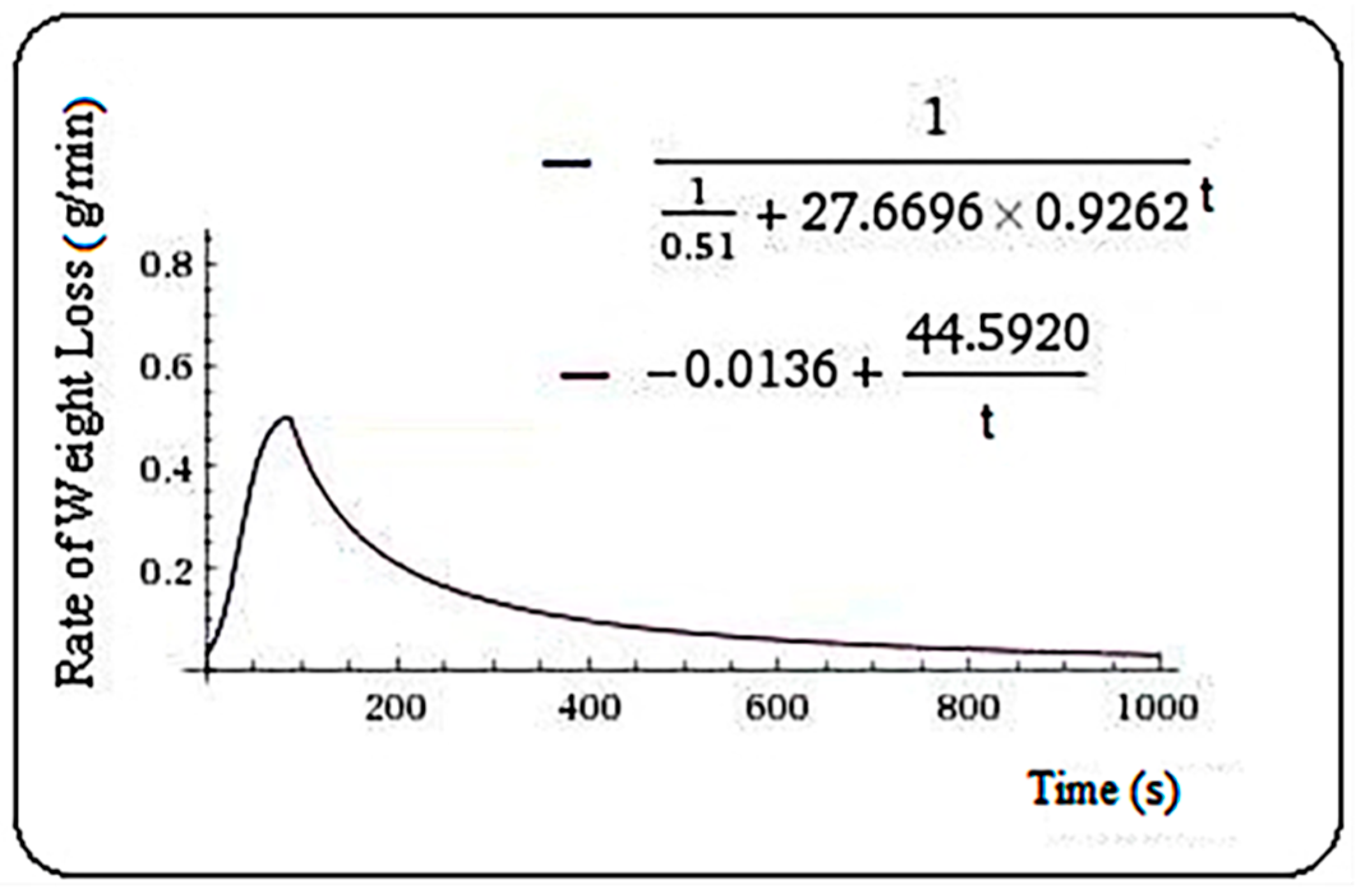
| a | b | u | Nettle | t2 | t1 |
|---|---|---|---|---|---|
| 27.6696 | 0.9262 | 0.51 | 80 | 10 | |
| I(t2) | I(t1) | total branch 1 (integral calculation) | total branch 1 (measurement) | Sig. | Rsq. |
| 41.00061 | 18.55301 | 0.37 | 0.41 | 0.000 | 0.987 |
| α | β | t2 | t1 | ||
| −0.0136 | 44.592 | 1190 | 80 | ||
| J(t2) | J(t1) | total branch 2 (integral calculation) | total branch 2 (measurement) | Sig. | Rsq. |
| 299.6035 | 194.3153 | 1.75 | 1.72 | 0.000 | 0.92 |
| a | b | u | Veronica | t2 | t1 |
|---|---|---|---|---|---|
| 51.086 | 0.9342 | 0.47 | 110 | 10 | |
| I(t2) | I(t1) | total branch 1 (integral calculation) | total branch 1 (measurement) | Sig. | Rsq. |
| 51.79227 | 22.49395 | 0.48 | 0.51 | 0.000 | 0.990 |
| α | β | t2 | t1 | ||
| 0.0147 | 49.2996 | 1420 | 110 | ||
| J(t2) | J(t1) | total branch 2 (integral calculation) | total branch 2 (measurement) | Sig. | Rsq. |
| 378.7108 | 233.3488 | 2.42 | 2.4 | 0.000 | 0.823 |
Publisher’s Note: MDPI stays neutral with regard to jurisdictional claims in published maps and institutional affiliations. |
© 2021 by the authors. Licensee MDPI, Basel, Switzerland. This article is an open access article distributed under the terms and conditions of the Creative Commons Attribution (CC BY) license (https://creativecommons.org/licenses/by/4.0/).
Share and Cite
Sala, F.; Herbei, M.V.; Rujescu, C. RWLMod—Potential Model to Study Plant Tolerance in Drought Stress Conditions. Plants 2021, 10, 2576. https://doi.org/10.3390/plants10122576
Sala F, Herbei MV, Rujescu C. RWLMod—Potential Model to Study Plant Tolerance in Drought Stress Conditions. Plants. 2021; 10(12):2576. https://doi.org/10.3390/plants10122576
Chicago/Turabian StyleSala, Florin, Mihai Valentin Herbei, and Ciprian Rujescu. 2021. "RWLMod—Potential Model to Study Plant Tolerance in Drought Stress Conditions" Plants 10, no. 12: 2576. https://doi.org/10.3390/plants10122576