
Species Distribution Pattern and Their Contribution in Plant Community Assembly in Response to Ecological Gradients of the Ecotonal Zone in the Himalayan Region

 , ,
, ,  ,
,  ,
,  , and
, and
Abstract
:1. Introduction
2. Materials and Methods
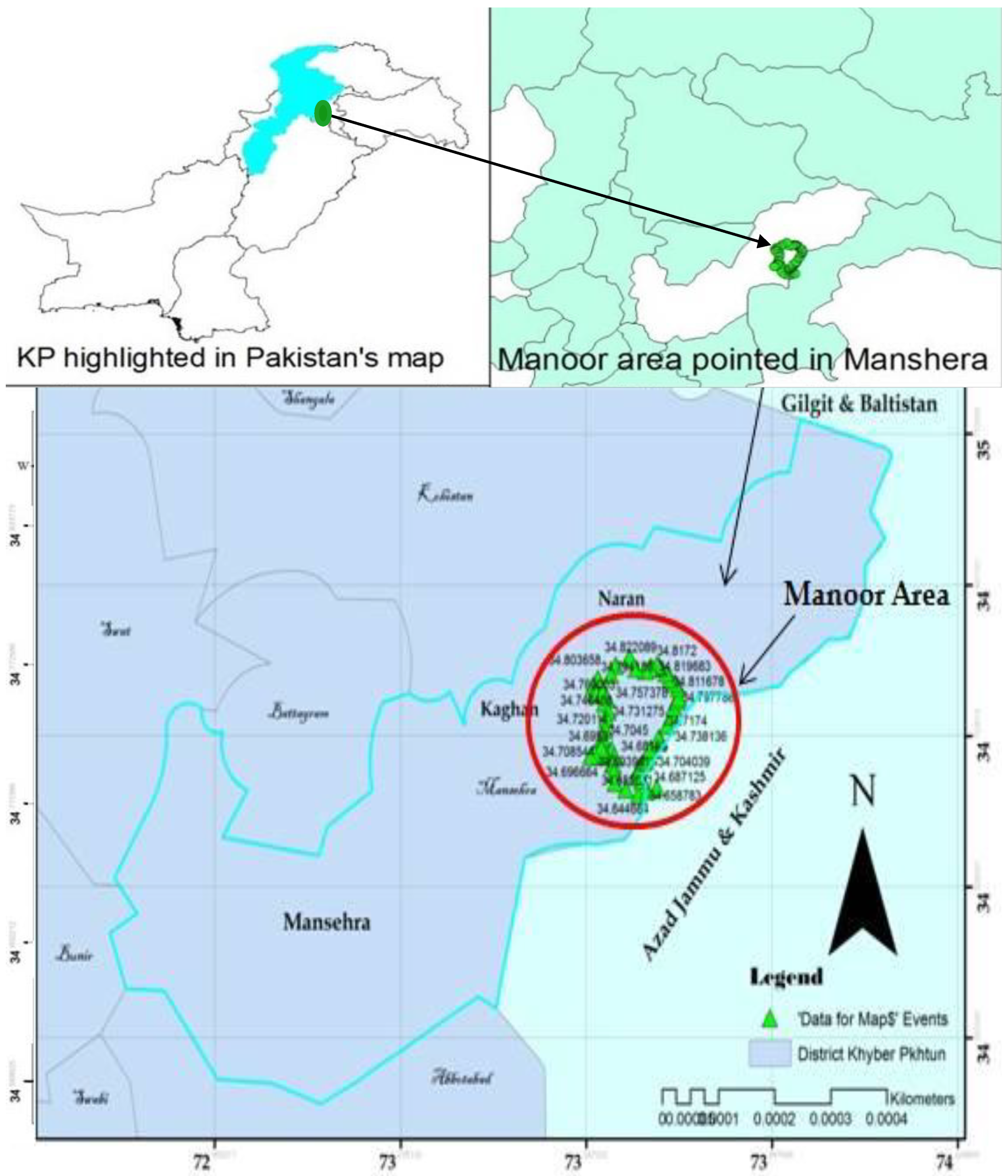
2.1. Study Area
2.2. Vegetation Sampling
2.3. Ecological Gradients
2.4. Data Analyses
3. Results
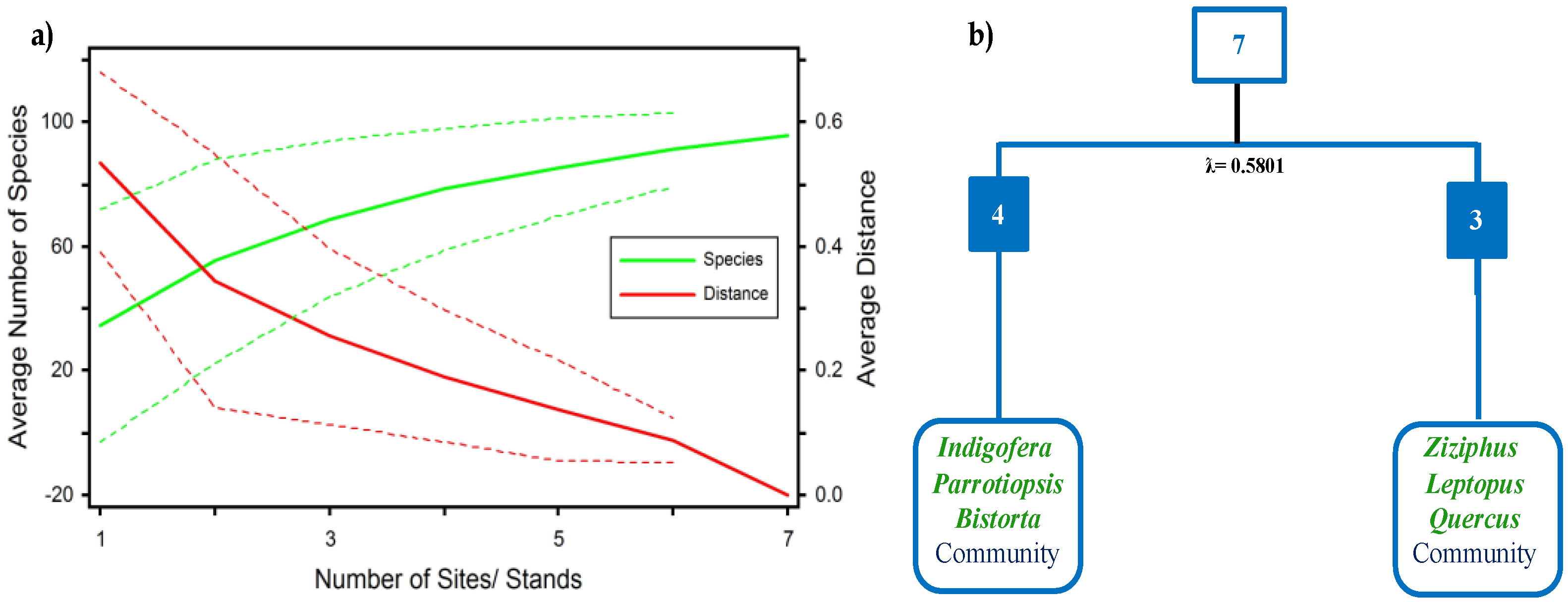
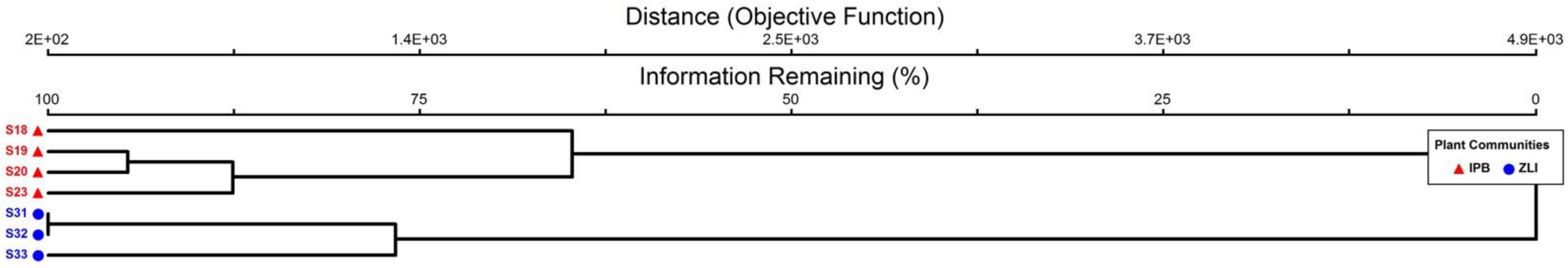
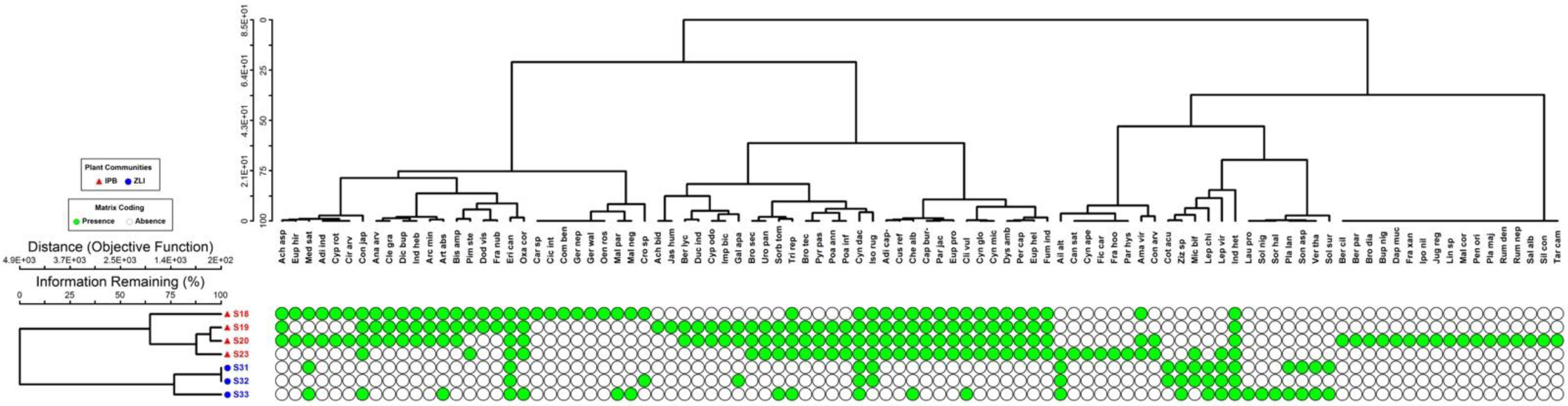
3.1. Vegetation Characterization
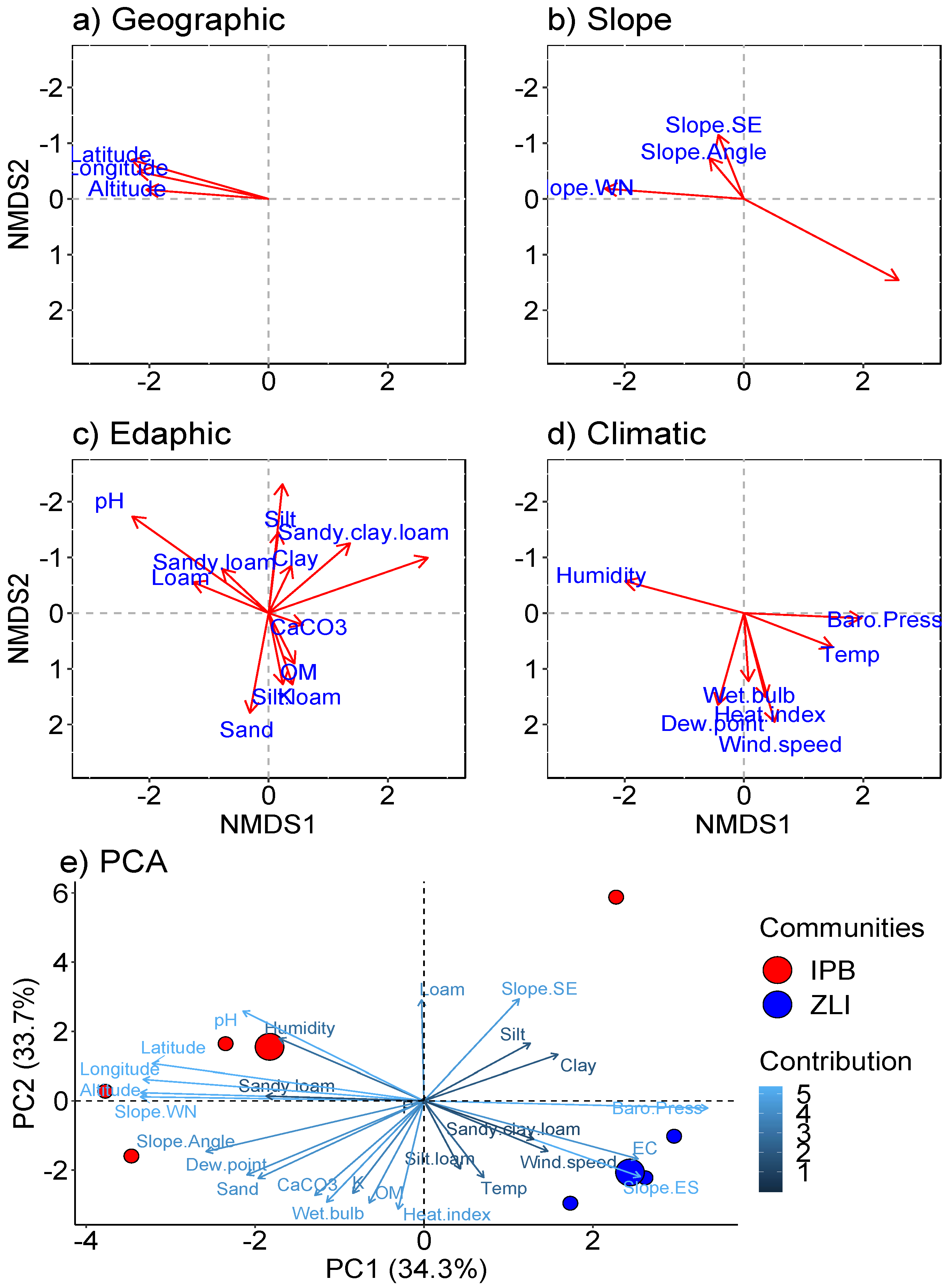
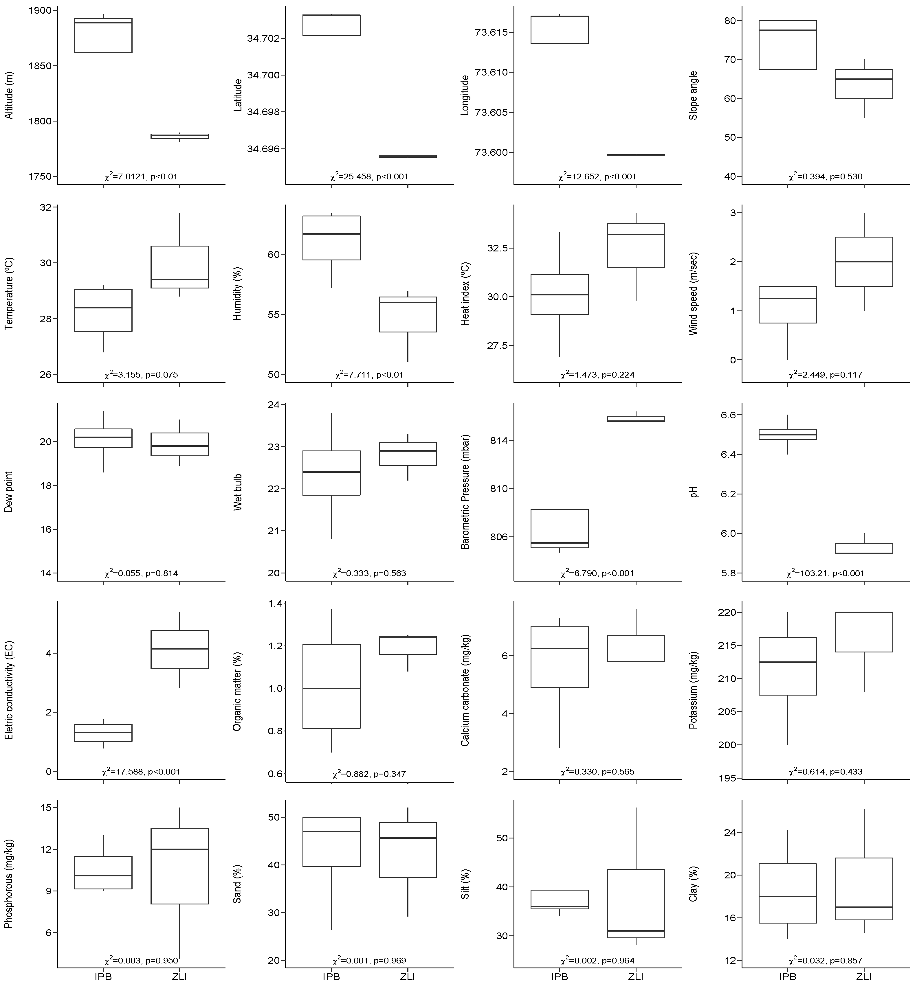
3.2. Vegetation along the Ecological Gradients
3.3. Analysis of Similarity (ANOSIM)
3.4. Significance Testing of Plant Communities in Relation to Studied Variables
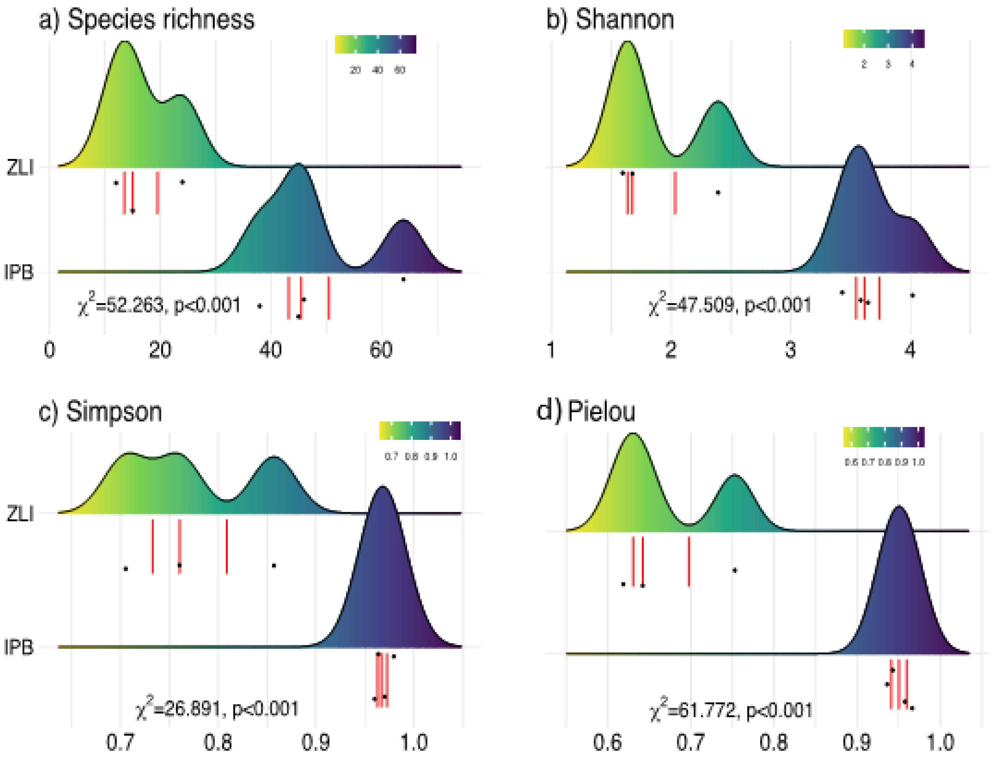
3.5. Species Richness and Diversity Indices
4. Discussion
5. Conclusions
Supplementary Materials
Author Contributions
Funding
Institutional Review Board Statement
Informed Consent Statement
Data Availability Statement
Acknowledgments
Conflicts of Interest
References
- Clements, F.E. Research Methods in Ecology; University Publ. Co.: Lincoln, NA, USA, 1905; p. 199. [Google Scholar]
- Casalini, A.I.; Bouza, P.J.; Bisigato, A.J. Geomorphology, soil and vegetation patterns in an arid ecotone. Catena 2019, 174, 353–361. [Google Scholar] [CrossRef]
- Attrill, M.; Rundle, S. Ecotone or Ecocline: Ecological Boundaries in Estuaries. Estuar. Coast. Shelf Sci. 2002, 55, 929–936. [Google Scholar] [CrossRef]
- Gonçalves, E.T.; Souza, A.F. Floristic variation in ecotonal areas: Patterns, determinants and biogeographic origins of sub-tropical forests in South America. Austral. Ecol. 2014, 39, 122–134. [Google Scholar] [CrossRef]
- Arellano, G.; Umaña, M.N.; Macía, M.J.; Loza, M.I.; Fuentes, A.; Cala, V.; Jørgensen, P.M. The role of niche overlap, environmental heterogeneity, landscape roughness and productivity in shaping species abundance distributions along the Amazon–Andes gradient. Glob. Ecol. Biogeogr. 2017, 26, 191–202. [Google Scholar]
- Frahm, J.-P.; Gradstein, S.R. An altitudinal zonation of tropical rain forests using byrophytes. J. Biogeogr. 1991, 18, 669. [Google Scholar] [CrossRef]
- Motiekaityte, V.; Motiekaityté, V. Conservation Diversity of Vascular Plants and their Communities in situ, applying the Conception of Ecosystem Pool. Ekologija 2006, 2, 1–7. [Google Scholar]
- Myers, N.; Mittermeier, R.A.; Mittermeier, C.G.; Da Fonseca, G.A.; Kent, J. Biodiversity hotspots for conservation priorities. Nature 2000, 403, 853–858. Available online: http://www.ncbi.nlm.nih.gov/pubmed/10706275 (accessed on 18 August 2021). [CrossRef]
- Shipley, B.; Keddy, P.A. The individualistic and community-unit concepts as falsifiable hypotheses. In Theory and Models in Vegetation Science; Springer: Dortmund, Germany, 1987; Volume 69, pp. 47–55. [Google Scholar] [CrossRef]
- Vleminckx, J.; Schimann, H.; Decaëns, T.; Fichaux, M.; Vedel, V.; Jaouen, G.; Roy, M.; Lapied, E.; Engel, J.; Dourdain, A.; et al. Coordinated community structure among trees, fungi and invertebrate groups in Amazonian rainforests. Sci. Rep. 2019, 9, 1–10. [Google Scholar] [CrossRef] [Green Version]
- Hu, A.; Wang, J.; Sun, H.; Niu, B.; Si, G.; Wang, J.; Yeh, C.-F.; Zhu, X.; Lu, X.; Zhou, J.; et al. Mountain biodiversity and ecosystem functions: Interplay between geology and contemporary environments. ISME J. 2020, 14, 931–944. [Google Scholar] [CrossRef] [PubMed]
- Kark, S. Ecotones and Ecological Gradients. In Ecological Systems; Springer Science and Business Media LLC: Berlin/Heidelberg, Germany, 2013; pp. 147–160. [Google Scholar]
- Erdős, L. On the terms related to spatial ecological gradients and boundaries. Acta Biol. Szeged. 2011, 55, 279–287. [Google Scholar]
- Kent, M.; Gill, W.J.; Weaver, R.E.; Armitage, R.P. Landscape and plant community boundaries in biogeography. Prog. Phys. Geogr. Earth Environ. 1997, 21, 315–353. [Google Scholar] [CrossRef]
- Vance, R.B. Odum. Fundamentals of Ecology (Book Review). Soc. Forces 1953, 32, 376. [Google Scholar]
- Ludwig, J.A.; Cornelius, J.M. Locating Discontinuities along Ecological Gradients. Ecology 1987, 68, 448–450. [Google Scholar] [CrossRef]
- Delgado-Mellado, N.; Larriba, M.; Navarro, P.; Rigual, V.; Ayuso, M.; García, J.; Rodríguez, F. Thermal stability of choline chloride deep eutectic solvents by TGA/FTIR-ATR analysis. J. Mol. Liq. 2018, 260, 37–43. [Google Scholar] [CrossRef]
- Hussain, M.; Khan, S.M.; Abd_Allah, E.F.; Ul Haq, Z.; Alshahrani, T.S.; Alqarawi, A.A.; Ur Rahman, I.; Iqbal, M.; Abdullah–Ahmad, H. Assessment of Plant communities and identification of indicator species of an ecotonal forest zone at durand line, district Kurram, Pakistan. Appl. Ecol. Environ. Res. 2019, 17, 6375–6396. [Google Scholar] [CrossRef]
- Rahman, I.U.; Afzal, A.; Iqbal, Z.; Bussmann, R.W.; Alsamadany, H.; Calixto, E.S.; Shah, G.M.; Kausar, R.; Shah, M.; Ali, N.; et al. Ecological gradients hosting plant communities in Himalayan subalpine pastures: Application of multivariate approaches to identify indicator species. Ecol. Inform. 2020, 60, 101162. [Google Scholar] [CrossRef]
- Rahman, I.U.; Afzal, A.; Iqbal, Z.; Abd Allah, E.F.; Alqarawi, A.A.; Calixto, E.S.; Ali, N.; Ijaz, F.; Kausar, R.; Alsubeie, M.S.; et al. Role of multivariate approaches in floristic diversity of Manoor Valley (Himalayan Region), Pakistan. Appl. Ecol. Environ. Res. 2019, 17, 1475–1498. [Google Scholar] [CrossRef]
- Rahman, I.U.; Afzal, A.; Iqbal, Z.; Ijaz, F.; Ali, N.; Asif, M.; Alam, J.; Majid, A.; Hart, R.; Bussmann, R.W. First insights into the floristic diversity, biological spectra and phenology of Manoor valley, Pakistan. Pakistan J. Bot. 2018, 50, 1113–1124. [Google Scholar]
- Rahman, I.U.; Ijaz, F.; Afzal, A.; Iqbal, Z.; Ali, N.; Khan, S.M. Contributions to the phytotherapies of digestive disorders: Traditional knowledge and cultural drivers of Manoor Valley, Northern Pakistan. J. Ethnopharmacol. 2016, 192, 30–52. [Google Scholar] [CrossRef]
- Rahman, I.U.; Afzal, A.; Iqbal, Z.; Hart, R.; Allah, E.F.A.; Hashem, A.; Alsayed, M.F.; Ijaz, F.; Ali, N.; Shah, M.; et al. Herbal teas and drinks: Folk medicine of the Manoor Valley, Lesser Himalaya, Pakistan. Plants 2019, 8, 581. [Google Scholar] [CrossRef] [Green Version]
- Buckland, S.T.; Anderson, D.R.; Burnham, K.P.; Laake, J.L.; Borchers, D.L.; Thomas, L. Introduction to Distance Sampling: Estimating Abundance of Biological Populations, 1st ed.; Oxford University Press: Oxford, UK, 2001. [Google Scholar]
- Buckland, S.T.; Anderson, D.R.; Burnham, K.P.; Laake, J.L.; Borchers, D.L.; Thomas, L. Advanced Distance Sampling; Oxford University Press Oxford: Oxford, UK, 2004; Volume 2. [Google Scholar]
- Buckland, S.; Newman, K.B.; Fernández, C.; Thomas, L.; Harwood, J. Embedding Population Dynamics Models in Inference. Stat. Sci. 2007, 22, 44–58. [Google Scholar] [CrossRef] [Green Version]
- Anderson, D.R.; Burnham, K.P.; Laake, J.L. Distance Sampling: Estimating Abundance of Biological Populations; Chapman & Hall: London, UK, 1993. [Google Scholar]
- Sprent, P.; Buckland, S.T.; Anderson, D.R.; Burnham, K.P.; Laake, J.L. Distance sampling-estimating abundance of biological populations. J. Appl. Ecol. 1994, 31, 789. [Google Scholar] [CrossRef]
- Le Moullec, M.; Pedersen, Å.Ø.; Yoccoz, N.; Aanes, R.; Tufto, J.; Hansen, B. Ungulate population monitoring in an open tundra landscape: Distance sampling versus total counts. Wildl. Biol. 2017, 2017. [Google Scholar] [CrossRef] [Green Version]
- Kent, M. Vegetation Description and Data Analysis: A Practical Approach, 2nd ed.; John Wiley & Sons: Hoboken, NJ, USA, 2012; ISBN 1119962390. [Google Scholar]
- Curtis, J.T.; McIntosh, R.P. The interrelations of certain analytic and synthetic phytosociological characters. Ecology 1950, 31, 434–455. [Google Scholar] [CrossRef]
- Ijaz, F. Biodiversity and Traditional Uses of Plants of Sarban Hills, Abbottabad. M.Phil. Thesis, Department of Botany, Hazara University, Manehra, Pakistan, 2014. [Google Scholar]
- Ijaz, F.; Rahman, I.U.; Iqbal, Z.; Alam, J.; Ali, N.; Khan, S.M. Ethno-Ecology of the Healing Forests of Sarban Hills, Abbottabad, Pakistan: An Economic and Medicinal Appraisal; Springer Science and Business Media LLC: Berlin/Heidelberg, Germany, 2018; pp. 675–706. [Google Scholar]
- Nasir, E.; Ali, S.I. Papilionaceae. In Flora West of Pakistan; Nasir, E., Ali, S.I., Eds.; National Herbarium: Karachi, Pakistan, 1971. [Google Scholar]
- Ali, S.I.; Nasir, Y.J. Flora of Pakistan; Department of Botany, University of Karachi, Karachi and National Herbarium: Islamabad, Pakistan, 1989. [Google Scholar]
- Ali, S.I.; Qaiser, M. Flora of Pakistan; Department of Botany, University of Karachi: Karachi, Pakistan, 1995. [Google Scholar]
- Haq, F.; Ahmad, H.; Iqbal, Z. Vegetation description and phytoclimatic gradients of subtropical forests of Nandiar Khuwar catchment District Battagram. Pak. J. Bot. 2015, 47, 1399–1405. [Google Scholar]
- Ravindranath, N.H.; Ostwald, M. Carbon Inventory Methods Handbook for Greenhouse Gas Inventory, Carbon Mitigation and Roundwood Production Projects; Springer Science and Business Media LLC: Berlin/Heidelberg, Germany, 2008. [Google Scholar]
- McLean, E.O. Soil pH and lime requirement. Methods Soil Anal. Part 2 Chem. Microbiol. Prop. 1983, 9, 199–224. [Google Scholar] [CrossRef]
- Wilson, M.J.; Bayley, S.E. Use of single versus multiple biotic communities as indicators of biological integrity in northern prairie wetlands. Ecol. Indic. 2012, 20, 187–195. [Google Scholar] [CrossRef] [Green Version]
- Nelson, D.W.; Sommers, L.E. Total Carbon, Organic Carbon, and Organic Matter. In Methods of Soil Analysis: Part 3 Chemical Methods; SSSA: Madison, WI, USA, 1996; Volume 5, pp. 961–1010. [Google Scholar]
- Soltanpour, P.N. Determination of Nutrient Availability and Elemental Toxicity by AB-DTPA Soil Test and ICPS. In Advances in Soil Science; Springer Science and Business Media LLC: Berlin/Heidelberg, Germany, 1991; pp. 165–190. [Google Scholar]
- Rahman, I.U.; Afzal, A.; Iqbal, Z.; Ijaz, F.; Khan, S.M.; Khan, S.A.; Shah, A.H.; Khan, K.; Ali, N. Influence of different nutrients application in nutrient deficient soil on growth and yield of onion. Bangladesh J. Bot. 2015, 44, 613–619. [Google Scholar] [CrossRef]
- Rahman, I.U.; Ijaz, F.; Afzal, A.; Iqbal, Z. Effect of foliar application of plant mineral nutrients on the growth and yield at-tributes of chickpea (Cicer arietinum L.) Under nutrient deficient soil conditions. Bangladesh J. Bot. 2017, 46, 111–118. [Google Scholar]
- Šmilauer, P.; Jan, L. Multivariate Analysis of Ecological Data Using CANOCO, 2nd ed.; Cambridge University Press: Cambridge, UK, 2014. [Google Scholar]
- Mayor, J.R.; Sanders, N.J.; Classen, A.; Bardgett, R.D.; Clement, J.-C.; Fajardo, A.; Lavorel, S.; Sundqvist, M.K.; Bahn, M.; Chisholm, C.; et al. Elevation alters ecosystem properties across temperate treelines globally. Nat. Cell Biol. 2017, 542, 91–95. [Google Scholar] [CrossRef] [Green Version]
- Kenkel, N.C. On selecting an appropriate multivariate analysis. Can. J. Plant Sci. 2006, 86, 663–676. [Google Scholar] [CrossRef] [Green Version]
- McCune, B.; Mefford, M. PC-ORD. Multivariate Analysis of Ecological Data. Version 6; MjM Software Design: Gleneden Beach, OR, USA, 2011. [Google Scholar]
- R Core Team R. A Language and Environment for Statistical Computing; R Founding Statistical Company: Vienna, Austria, 2013. [Google Scholar]
- Bano, S.; Khan, S.M.; Alam, J.; Alqarawi, A.A.; Abd_Allah, E.F.; Ahmad, Z.; Rahman, I.U.; Ahmad, H.; Aldubise, A.; Hashem, A. Eco-Floristic studies of native plants of the Beer Hills along the Indus River in the districts Haripur and Abbottabad, Pakistan. Saudi J. Biol. Sci. 2018, 25, 801–810. [Google Scholar] [CrossRef] [PubMed]
- Haq, F.; Ahmad, H.; Iqbal, Z.; Alam, M.; Aksoy, A. Multivariate approach to the classification and ordination of the forest ecosystem of Nandiar valley western Himalayas. Ecol. Indic. 2017, 80, 232–241. [Google Scholar] [CrossRef]
- Hill, M.O. TWINSPAN: A FORTRAN Program for Arranging Multivariate Data in an Ordered Two-Way Table by Classification of the Individuals and Attributes; Cornell Univ.: Ithaca, NY, USA, 1979. [Google Scholar]
- Terzi, M.; Bogdanović, S.; D’Amico, F.S.; Jasprica, N. Rare plant communities of the Vis Archipelago (Croatia). Bot. Lett. 2019, 167, 241–254. [Google Scholar] [CrossRef]
- Oksanen, J.; Blanchet, F.G.; Friendly, M.; Kindt, R.; Legendre, P.; McGlinn, D.; Minchin, P.R.; O’Hara, R.B.; Simpson, G.L.; Solymos, P.; et al. The Vegan package. Community Ecol. Package 2007, 10, 719. [Google Scholar]
- Fox, J.; Weisberg, S. An R Companion to Applied Regression; Sage Publications: Thousand Oaks, CA, USA, 2018. [Google Scholar]
- Rahman, I.U. Ecophysiological Plasticity and Ethnobotanical Studies in Manoor Area, Kaghan Valley, Pakistan. Ph.D. Thesis, Department of Botany, Hazara University, Mansehra, Pakistan, 2020. [Google Scholar]
- Khan, S.M. Plant Communities and Vegetation Ecosystem Services in the Naran Valley, Western Himalaya. Ph.D. Thesis, University of Leicester, Leicester, UK, 2012. [Google Scholar]
- Hufkens, K.; Scheunders, P.; Ceulemans, R. Ecotones in vegetation ecology: Methodologies and definitions revisited. Ecol. Res. 2009, 24, 977–986. [Google Scholar] [CrossRef]
- Luo, Z.; Tang, S.; Li, C.; Fang, H.; Hu, H.; Yang, J.; Ding, J.; Jiang, Z. Environmental Effects on Vertebrate Species Richness: Testing the Energy, Environmental Stability and Habitat Heterogeneity Hypotheses. PLoS ONE 2012, 7, e35514. [Google Scholar] [CrossRef] [Green Version]
- Yang, Z.; Liu, X.; Zhou, M.; Ai, D.; Wang, G.; Wang, Y.; Chu, C.; Lundholm, J.T. The effect of environmental heterogeneity on species richness depends on community position along the environmental gradient. Sci. Rep. 2015, 5, 15723. [Google Scholar] [CrossRef]
- Digby, P.G.N.; Kempton, R.A. Multivariate Analysis of Ecological Communities; Springer Science & Business Media: Berlin/Heidelberg, Germany, 2012; Volume 5, ISBN 9400931352. [Google Scholar]
- Biondi, E.; Feoli, E.; Zuccarello, V. Modelling environmental responses of plant associations: A review of some critical concepts in vegetation study. Crit. Rev. Plant Sci. 2004, 23, 149–156. [Google Scholar] [CrossRef]
- James, F.C.; McCulloch, C.E. Multivariate analysis in ecology and systematics: Panacea or Pandora’s box? Annu. Rev. Ecol. Syst. 1990, 21, 129–166. [Google Scholar] [CrossRef]
- Beals, M.L. Understanding community structure: A data-driven multivariate approach. Oecologia 2006, 150, 484–495. [Google Scholar] [CrossRef]
- Glatthorn, J.; Feldmann, E.; Tabaku, V.; Leuschner, C.; Meyer, P. Classifying development stages of primeval European beech forests: Is clustering a useful tool? BMC Ecol. 2018, 18, 47. [Google Scholar] [CrossRef] [Green Version]
- Dufrêne, M.; Legendre, P. Species assemblages and indicator species: The need for a flexible asymmetrical approach. Ecol. Monogr. 1997, 67, 345–366. [Google Scholar] [CrossRef]
- Paudel, P.K.; Sipos, J.; Brodie, J.F. Threatened species richness along a Himalayan elevational gradient: Quantifying the influ-ences of human population density, range size, and geometric constraints. BMC Ecol. 2018, 18, 1–8. [Google Scholar] [CrossRef] [Green Version]
- Anderson, M.J.; Ellingsen, K.E.; McArdle, B.H. Multivariate dispersion as a measure of beta diversity. Ecol. Lett. 2006, 9, 683–693. [Google Scholar] [CrossRef]
- Haq, F.; Ahmad, H.; Iqbal, Z. Vegetation composition and ecological gradients of subtropical-moist temperate Ecotonal forests of Nandiar Khuwar Catchment, Pakistan. Bangladesh J. Bot. 2015, 44, 267–276. [Google Scholar] [CrossRef]
- Khan, S.M.; Harper, D.M.; Page, S.; Ahmad, H. Species and community diversity of vascular flora along environmental gra-dient in Naran Valley: A multivariate approach through indicator species analysis. Pak. J. Bot. 2011, 43, 2337–2346. [Google Scholar]
- Klanderud, K.; Birks, H.J.B. Recent increases in species richness and shifts in altitudinal distributions of Norwegian mountain plants. Holocene 2003, 13, 1–6. [Google Scholar] [CrossRef] [Green Version]
- Odland, A.; Birks, H.J.B. The altitudinal gradient of vascular plant richness in Aurland, western Norway. Ecography (Cop.). Ecography 1999, 22, 548–566. [Google Scholar] [CrossRef]
- Weckström, J.; Korhola, A. Patterns in the distribution, composition and diversity of diatom assemblages in relation to eco-climatic factors in Arctic Lapland. J. Biogeogr. 2001, 28, 31–45. [Google Scholar] [CrossRef]
- Shaheen, H.; Ullah, Z.; Khan, S.M.; Harper, D.M. Species composition and community structure of western Himalayan moist temperate forests in Kashmir. For. Ecol. Manag. 2012, 278, 138–145. [Google Scholar] [CrossRef]
- Sahney, S.; Benton, M.J.; Ferry, P.A. Links between global taxonomic diversity, ecological diversity and the expansion of ver-tebrates on land. Biol. Lett. 2010, 6, 544–547. [Google Scholar] [CrossRef] [PubMed] [Green Version]
- Benton, M.J. The origins of modern biodiversity on land. Philos. Trans. R. Soc. B Biol. Sci. 2010, 365, 3667–3679. [Google Scholar] [CrossRef]
- Smith, M.; Facelli, J.; Cavagnaro, T. Interactions between soil properties, soil microbes and plants in remnant-grassland and old-field areas: A reciprocal transplant approach. Plant Soil 2018, 433, 127–145. [Google Scholar] [CrossRef]
- Allen, C.D.; Breshears, D.D. Drought-induced shift of a forest-woodland ecotone: Rapid landscape response to climate variation. Proc. Natl. Acad. Sci. USA 1998, 95, 14839–14842. [Google Scholar] [CrossRef] [Green Version]
- Crumley, C.L. Analyzing historic ecotonal shifts. Ecol. Appl. 1993, 3, 377–384. [Google Scholar] [CrossRef]
- Neilson, R.P. Transient ecotone response to climatic change: Some conceptual and modelling approaches. Ecol. Appl. 1993, 3, 385–395. [Google Scholar] [CrossRef]


| Species | Abbreviations | NMDS1 | NMDS2 | r2 | Pr(>r) |
|---|---|---|---|---|---|
| Achyranthes aspera L. | Ach.asp | −0.96987 | 0.24364 | 0.4507 | 0.257 |
| Achyranthes bidentata Blume | Ach.bid | −0.70128 | −0.71289 | 0.1373 | 1.000 |
| Adiantum capillus-veneris L. | Adi.cap−ven | −0.96337 | −0.26818 | 0.8058 | 0.039 |
| Aesculus indica (Wall. ex Camb.) Hook. | Adi.ind | −0.91470 | 0.40413 | 0.3475 | 0.372 |
| Ailanthus altissima (Mill.) Swingle | Ail.alt | −0.07487 | 0.99719 | 0.0154 | 0.968 |
| Amaranthus viridis L. | Ama.vir | −0.78624 | −0.61792 | 0.4079 | 0.356 |
| Anagallis arvensis L. | Ana.arv | −0.99174 | 0.12829 | 0.5186 | 0.242 |
| Arctium minus (Hill) Benh. | Arc.min | −0.99793 | 0.06433 | 0.5744 | 0.187 |
| Artemisia absinthium L. | Art.abs | −0.76707 | 0.64156 | 0.6196 | 0.155 |
| Bergenia ciliata (Haw.) Sternb. | Ber.cil | −0.93351 | −0.35856 | 0.1997 | 0.558 |
| Berberis lycium Royle | Ber.lyc | −0.86966 | −0.49365 | 0.3704 | 0.280 |
| Berberis parkeriana C.K. Schneid. | Ber.par | −0.93351 | −0.35856 | 0.1997 | 0.558 |
| Bistorta amplexicaulis (D. Don) Greene | Bis.amp | −0.91497 | 0.40353 | 0.3037 | 0.434 |
| Bromus diandrus Roth. | Bro.dia | −0.93351 | −0.35856 | 0.1997 | 0.558 |
| Bromus secalinus L. | Bro.sec | −0.69951 | −0.71463 | 0.6587 | 0.078 |
| Bromus tectorum L. | Bro.tec | −0.66386 | −0.74786 | 0.6800 | 0.080 |
| Bupleurum nigrescens E. Nasir | Bup.nig | −0.93351 | −0.35856 | 0.1997 | 0.558 |
| Cannabis sativa L. | Can.sat | −0.35050 | −0.93656 | 0.1671 | 0.701 |
| Capsella bursa-pastoris (L.) Medik. | Cap.bur−pas | −0.91592 | −0.40136 | 0.7852 | 0.067 |
| Carex sp. | Car.sp | −0.61623 | 0.78757 | 0.1488 | 0.859 |
| Chenopodium album L. | Che.alb | −0.99837 | −0.05713 | 0.5975 | 0.160 |
| Cichorium intybus L. | Cic.int | −0.61623 | 0.78757 | 0.1488 | 0.859 |
| Cirsium arvense (L.) Scop. | Cir.arv | −0.89265 | 0.45075 | 0.3329 | 0.437 |
| Clematis grata Wall. | Cle.gra | −0.98884 | 0.14896 | 0.4495 | 0.313 |
| Clinopodium vulgare L. | Cli.vul | −0.95549 | −0.29502 | 0.8765 | 0.025 |
| Commelina benghalensis L. | Com.ben | −0.61623 | 0.78757 | 0.1488 | 0.859 |
| Convolvulus arvensis L. | Con.arv | −0.54123 | −0.84088 | 0.3380 | 0.380 |
| Conyza japonica (Thunb.) Less. ex Less. | Con.jap | −0.82955 | 0.55844 | 0.5936 | 0.154 |
| Cotoneaster acuminatus Wall. ex Lindl. | Cot.acu | 0.69116 | −0.72270 | 0.9339 | 0.031 |
| Crotalaria sp. | Cro.sp | 0.81696 | −0.57670 | 0.0080 | 0.970 |
| Cuscuta reflexa Roxb. | Cus.ref | −0.97647 | −0.21564 | 0.6624 | 0.118 |
| Cynoglossum apenninum L. | Cyn.ape | −0.35050 | −0.93656 | 0.1671 | 0.701 |
| Cynodon dactylon (L.) Pers. | Cyn.dac | −0.99873 | 0.05040 | 0.5807 | 0.180 |
| Cynoglossum glochidiatum Wall. ex Benth. | Cyn.glo | −0.84752 | −0.53076 | 0.7874 | 0.064 |
| Cynoglossum microglochin Benth. | Cyn.mic | −0.84104 | −0.54098 | 0.8332 | 0.040 |
| Cyperus odoratus L. | Cyp.odo | −0.79409 | −0.60781 | 0.3201 | 0.430 |
| Cyperus rotundus L. | Cyp.rot | −0.90457 | 0.42633 | 0.3411 | 0.397 |
| Daphne mucronata Royle | Dap.muc | −0.93351 | −0.35856 | 0.1997 | 0.558 |
| Dicliptera bupleuroides Nees | Dic.bup | −0.96871 | 0.24818 | 0.4817 | 0.265 |
| Dodonaea viscosa (L.) Jacq. | Dod.vis | −0.99805 | −0.06247 | 0.2555 | 0.583 |
| Duchesnea indica (Andx) Fake. | Duc.ind | −0.84188 | −0.53966 | 0.3961 | 0.256 |
| Dysphania ambrosioides (L.) Mosyakin & Clemants | Dys.amb | −0.90846 | −0.41798 | 0.9613 | 0.013 |
| Erigeron canadensis L. | Eri.can | −0.21391 | 0.97685 | 0.5741 | 0.173 |
| Euphorbia helioscopia L. | Eup.hel | −0.93448 | −0.35602 | 0.9337 | 0.012 |
| Euphorbia hirta L. | Eup.hir | −0.94701 | 0.32120 | 0.3630 | 0.364 |
| Euphorbia prostrata Ait. | Eup.pro | −0.89409 | −0.44789 | 0.6637 | 0.105 |
| Ficus carica L. | Fic.car | −0.35050 | −0.93656 | 0.1671 | 0.701 |
| Fraxinus hookeri Wenz. | Fra.hoo | −0.35050 | −0.93656 | 0.1671 | 0.701 |
| Fragaria nubicola (Hook. f.) Lindl. ex Lacaita | Fra.nub | −0.98608 | 0.16625 | 0.2652 | 0.557 |
| Fraxinus xanthoxyloides (G. Don) DC. | Fra.xan | −0.93351 | −0.35856 | 0.1997 | 0.558 |
| Fumaria indica (Hausskn) Pugsley | Fum.ind | −0.81941 | −0.57321 | 0.9588 | 0.007 |
| Galium aparine L. | Gal.apa | −0.41051 | −0.91186 | 0.2183 | 0.625 |
| Geranium nepalense Sweet. | Ger.nep | −0.61623 | 0.78757 | 0.1488 | 0.859 |
| Geranium wallichianum D. Don ex Sweet | Ger.wal | −0.61623 | 0.78757 | 0.1488 | 0.859 |
| Impatiens bicolor Royle. | Imp.bic | −0.79600 | −0.60529 | 0.3248 | 0.430 |
| Indigofera hebepetala Baker | Ind.heb | −0.94517 | 0.32659 | 0.4344 | 0.284 |
| Indigofera heterantha Brandis | Ind.het | 0.30346 | 0.95285 | 0.2066 | 0.644 |
| Ipomoea nil (L.) Roth | Ipo.nil | −0.93351 | −0.35856 | 0.1997 | 0.558 |
| Isodon rugosus (Wall. ex Benth.) Codd | Iso.rug | −0.36383 | −0.93146 | 0.6163 | 0.137 |
| Jasminum humile L. | Jas.hum | −0.70128 | −0.71289 | 0.1373 | 1.000 |
| Juglans regia L. | Jug.reg | −0.93351 | −0.35856 | 0.1997 | 0.558 |
| Launaea procumbens (Roxb.) Ramayya and Rajagopal | Lau.pro | 0.11700 | 0.99313 | 0.8884 | 0.148 |
| Leptopus chinensis (Bunge) Pojark. | Lep.chi | 0.94983 | 0.31278 | 0.9680 | 0.015 |
| Leptodermis virgata Edgew. ex Hook.F. | Lep.vir | 0.60228 | −0.79828 | 0.3181 | 0.457 |
| Lindelofia sp. | Lin.sp | −0.93351 | −0.35856 | 0.1997 | 0.558 |
| Malvastrum coromandelianum (L.) Garcke | Mal.cor | −0.93351 | −0.35856 | 0.1997 | 0.558 |
| Malva parviflora L | Mal.par | −0.13602 | 0.99071 | 0.4815 | 0.224 |
| Malva neglecta Wallr. | Mal.neg | −0.21533 | 0.97654 | 0.3408 | 0.295 |
| Medicago sativa L. | Med.sat | −0.67170 | 0.74083 | 0.3808 | 0.324 |
| Micromeria biflora (Ham.) Bth. | Mic.bif | 0.50585 | −0.86262 | 0.8617 | 0.044 |
| Oenothera rosea L. Her ex Aiton | Oen.ros | −0.61623 | 0.78757 | 0.1488 | 0.859 |
| Oxalis corniculata L. | Oxa.cor | −0.70137 | 0.71279 | 0.5950 | 0.189 |
| Parthenium hysterophorus L. | Par.hys | −0.35050 | −0.93656 | 0.1671 | 0.701 |
| Parrotiopsis jacquemontiana (Decne.) Rehder | Par.jac | −0.93944 | −0.34272 | 0.6925 | 0.099 |
| Pennisetum orientale Rich. | Pen.ori | −0.93351 | −0.35856 | 0.1997 | 0.558 |
| Persicaria capitata (Buch.-Ham. ex D.Don) H.Gross | Per.cap | −0.89091 | −0.45418 | 0.9782 | 0.019 |
| Pimpinella stewartii (Dunn) Nasir | Pim.ste | −0.99881 | 0.04881 | 0.3136 | 0.413 |
| Plantago lanceolata L. | Pla.lan | 0.18423 | 0.98288 | 0.8884 | 0.045 |
| Plantago major L. | Pla.maj | −0.93351 | −0.35856 | 0.1997 | 0.558 |
| Poa annua L. | Poa.ann | −0.67556 | −0.73730 | 0.5850 | 0.132 |
| Poa infirma Kunth | Poa.inf | −0.64465 | −0.76448 | 0.5003 | 0.232 |
| Pyrus pashia Buch.-Ham. ex D.Don | Pyr.pas | −0.64295 | −0.76591 | 0.6690 | 0.094 |
| Quercusincana Bartram | Que.inc | 0.74983 | 0.35278 | 0.9480 | 0.035 |
| Rumex dentatus L. | Rum.den | −0.93351 | −0.35856 | 0.1997 | 0.558 |
| Rumex nepalensis Sprenge | Rum.nep | −0.93351 | −0.35856 | 0.1997 | 0.558 |
| Salix alba L. | Sal.alb | −0.93351 | −0.35856 | 0.1997 | 0.558 |
| Silene conoidea L. | Sil.con | −0.93351 | −0.35856 | 0.1997 | 0.558 |
| Solanum nigrum L. | Sol.nig | 0.11700 | 0.99313 | 0.8884 | 0.148 |
| Solanum surattense Burm F. | Sol.sur | 0.32179 | 0.94681 | 0.7930 | 0.089 |
| Sonchus asper (L.) Hill | Son.asp | 0.18595 | 0.98256 | 0.8879 | 0.045 |
| Sorghum halepense (L.) Pers. | Sor.hal | 0.11700 | 0.99313 | 0.8884 | 0.148 |
| Sorbaria tomentosa (Lindl.) Rehder | Sorb.tom | −0.99934 | −0.03641 | 0.4449 | 0.309 |
| Taraxacum officinale aggr. F.H. Wigg. | Tar.off | −0.93351 | −0.35856 | 0.1997 | 0.558 |
| Trifolium repens L. | Tri.rep | −0.96524 | −0.26135 | 0.8350 | 0.024 |
| Urochloa panicoides P. Beauv. | Uro.pan | −0.69247 | −0.72145 | 0.6679 | 0.082 |
| Verbascum thapsus L. | Ver.tha | 0.15572 | 0.98780 | 0.8935 | 0.045 |
| Ziziphus sp. | Ziz.sp | 0.91809 | −0.39636 | 0.9309 | 0.014 |
Publisher’s Note: MDPI stays neutral with regard to jurisdictional claims in published maps and institutional affiliations. |
© 2021 by the authors. Licensee MDPI, Basel, Switzerland. This article is an open access article distributed under the terms and conditions of the Creative Commons Attribution (CC BY) license (https://creativecommons.org/licenses/by/4.0/).
Share and Cite
Rahman, I.U.; Afzal, A.; Iqbal, Z.; Hashem, A.; Al-Arjani, A.-B.F.; Alqarawi, A.A.; Abd_Allah, E.F.; Abdalla, M.; Calixto, E.S.; Sakhi, S.; et al. Species Distribution Pattern and Their Contribution in Plant Community Assembly in Response to Ecological Gradients of the Ecotonal Zone in the Himalayan Region. Plants 2021, 10, 2372. https://doi.org/10.3390/plants10112372
Rahman IU, Afzal A, Iqbal Z, Hashem A, Al-Arjani A-BF, Alqarawi AA, Abd_Allah EF, Abdalla M, Calixto ES, Sakhi S, et al. Species Distribution Pattern and Their Contribution in Plant Community Assembly in Response to Ecological Gradients of the Ecotonal Zone in the Himalayan Region. Plants. 2021; 10(11):2372. https://doi.org/10.3390/plants10112372
Chicago/Turabian StyleRahman, Inayat Ur, Aftab Afzal, Zafar Iqbal, Abeer Hashem, Al-Bandari Fahad Al-Arjani, Abdulaziz A. Alqarawi, Elsayed Fathi Abd_Allah, Mohnad Abdalla, Eduardo Soares Calixto, Shazia Sakhi, and et al. 2021. "Species Distribution Pattern and Their Contribution in Plant Community Assembly in Response to Ecological Gradients of the Ecotonal Zone in the Himalayan Region" Plants 10, no. 11: 2372. https://doi.org/10.3390/plants10112372