Influences of the Shadow Inventory on a Landslide Susceptibility Model

Abstract

A landslide inventory serves as the basis for assessing landslide susceptibility, hazard, and risk. It is generally prepared from optical imagery acquired from spaceborne or airborne platforms, in which shadows are inevitably found in mountainous areas. The influences of shadow inventory on a landslide susceptibility model (LSM), however, have not been investigated systematically. This paper employs both the shadow and landslide inventories prepared from eleven Formosat-2 annual images from the I-Lan area in Taiwan acquired from 2005 to 2016, using a semiautomatic expert system. A standard LSM based on the geometric mean of multivariables was used to evaluate the possible errors incurred by neglecting the shadow inventory. The results show that the LSM performance was significantly improved by 49.21% for the top 1% of the most highly susceptible area and that the performance decreased gradually by 15.25% for the top 10% most highly susceptible areas and 9.71% for the top 20% most highly susceptible areas. Excluding the shadow inventory from the calculation of landslide susceptibility index reveals the real contribution of each factor. They are crucial in optimizing the coefficients of a nondeterministic geometric mean LSM, as well as in deriving the threshold of a landslide hazard early warning system.

1. Introduction

A landslide inventory is a detailed register of the distribution and characteristics of past landslides [1]. It serves as the basis for assessing landslide susceptibility, hazard, and risk [2,3] and plays an essential role in landslide susceptibility models (LSMs) that predict landslides on the basis of past conditions [4,5,6,7,8,9,10,11]. A landslide inventory is generally prepared from optical imagery that is acquired from spaceborne or airborne platforms [12]. Because most landslides occur in mountainous areas, where the optical imagery is usually acquired while the sun is not in the nadir direction, so shadows are inevitably found as main features in an optical imagery of mountainous areas [13]. In Taiwan, for example, shadows can occupy as much as 30% of an entire image acquired in winter over a mountainous area. It is therefore necessary to employ a sound approach to detecting and excluding shadowy areas from an optical image before further analysis is performed.

Shahtahmassebi et al. [14] provided a comprehensive review of shadow detection and summarized four major techniques: thresholding, modeling, invariant color models, and shadow relief. Considering the advantages of speed and simplicity, they pointed out that thresholding techniques have become more and more important, even though cloud shadows and topographic shadows are always difficult to discriminate by specifying a simple threshold value. On the other hand, invariant color models are more sensitive to various types of shadows. Several approaches have been proposed to accurately delineate shadowy areas by projecting red-green-blue colors onto the hue-saturation-lightness components, such as the shadow index proposed by Ma et al. [15]. As a result, it is now feasible to prepare both the shadow and landslide inventories simultaneously from one optical image. From the point of view of an LSM, the question is whether it is necessary to spend the extra effort required to prepare a shadow inventory.

2. Study Area and Satellite Images

To investigate the influence of shadows on the LSM, I-Lan was selected as the study area for its steep topography and frequent disasters of landslide. I-Lan is located in the northeastern part of Taiwan, where the elevation plunges significantly from the Central Mountain in the southwest (≈2000 m above sea level (a.s.l) to the I-Lan plain in the northeast (≈10–100 m a.s.l), over a distance of just 30 km. Typhoons affect the southern part of Taiwan during the fall season. After converging in this region, their counterclockwise winds are further intensified by the northeasterly monsoon. Extreme rainfall is often recorded on the windward side, and consequently, many landslides have been triggered in this area. Taiwan’s Forestry Bureau funded three multiyear projects that employed the annual composite of Formosat-2 images collected between 2005 and 2016 to generate a detailed landslide inventory [16,17]. All Formosat-2 imagery was preprocessed using the Formosat-2 automatic image processing system (F-2 AIPS) [18], which is able to digest the raw Gerald format data, apply the basic radiometric and geometric correction, and can conduct rigorous band-to-band coregistration [19], automatic orthorectification [20], multitemporal image geometrical registration [21], multitemporal image radiometric normalization [22], spectral summation intensity modulation pan-sharpening [19], edge enhancement, and adaptive contrast enhancement, and the absolute radiometric calibration [23]. The main consideration in image selection is cloud coverage, so cloudless scenes collected in the winter are usually selected. Because there were cases of rapid response mapping significant landslides triggered by the extreme rainfall from Typhoon Morakot in August of 2009, most of the available aftermath images were also acquired in the winter of 2009 or in the spring of 2010. During that period of time, the sun elevation was low in the subtropical zone, when shadows could occupy as high as 30% of an entire image over a mountainous area. A standard false color image of I-Lan taken by Formosat-2 on 24 August 2009 is given in Figure 1a as an example, where both the landslide inventory and shadow inventory were prepared using a semiautomatic expert system [24] and masked as yellow and white polylines, respectively. Note that the thresholds of the shadows and landslides were both determined in a semiautomatic fashion and that there is no way to differentiate among a partially-shaded topography shadow, a completely-dark topography shadow, and a cloud shadow. The union of all landslide inventories (yellow polygons) and shadow inventories (white polygons) derived from the annual Formosat-2 imagery (2005–2016) are given in Figure 1b. Note that a map of Taiwan with an annotation of study area is also given in Figure 1a to illustrate the geographic location of I-Lan.

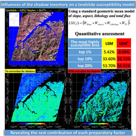
After excluding the river channel and those regions outside the study area (annotated in blue), the area ratios of the landslide inventory and shadow inventory are 3.9% and 34.1%, respectively. The lithology map was provided by the Central Geological Survey (CGS) of Taiwan (1/50,000 scale), while the slope, aspect, and total flux (TF) were calculated from a 5-m resolution digital elevation model (DEM), which was produced and made available by the Ministry of Interior Affairs of Taiwan (see Figure 2 in [25]). Note that TF considers the topography and hydrology conditions upstream of each gridded data cell and represents the total flux of water in the stream, which is strongly associated with the occurrence of landslides and is a good preparatory factor for LSM [25]. Liu et al. [25] demonstrated that drainage distance factor, defined as concentric multiringed buffer zones based on the distance of each cell from the main stream, may not be an accurate factor to represent the influence of neighboring cells. Because it may not properly represent the flux of water, likely responsible for the failure of slopes adjacent to streams.

3. Landslide Susceptibility Model

A standard LSM based on the geometric mean of multivariables, including a newly introduced region-based preparatory TF factor, was developed to map the landslide susceptibility in I-Lan [25,26]. This LSM can be used to predict landslides by weighting various preparatory factors pf [27] according to their contributions, and to compute a landslide susceptibility index (LSI) using the geometric mean model [28,29].

$$LSI(j)={\left({\displaystyle \prod _{k=1}^m{W}_{p{f}_k(i_k)}}\right)}^{\frac{1}{m}}$$

(1)

where j represents each cell of gridded raster data and the number of pf employed in the LSI is m. The frequency ratio method is used to weight pf values by the landslide inventory, as seen in the literature (e.g., [29,30,31,32]). The frequency ratio can be replaced by an area ratio under the assumption that all types of landslide events are covered by the landslide inventory. For each pf, the area ratio of each interval AR_pf(i) is defined as:

$$A{R}_{pf(i)}\equiv \frac{A_{pf(i)}}{A_t}=\frac{A_{pf(i)}}{{\displaystyle \sum _{i=1}^n{A}_{pf(i)}}}$$

(2)

where n specifies a fixed number of intervals (zones). Note that the area of pf at interval i is A_pf(i), and the total area of the study area is A_t. At each interval, the landslide ratio LR_pf(i) is therefore defined as the area ratio of

$$L{R}_{pf(i)}\equiv \frac{L_{pf(i)}}{L_t}=\frac{L_{pf(i)}}{{\displaystyle \sum _{i=1}^n{L}_{pf(i)}}},$$

(3)

where L_pf(i) is the landslide area of pf at interval i. L_t is the total landslide area. Because all landslides are delineated on Formosat-2 imagery outside shadowy areas, there is no intersection between the landslide and the shadow inventories. The weight of pf at interval i can be defined as the frequency ratio.

$$W_{pf(i)}\equiv \frac{L{R}_{pf(i)}}{A{R}_{pf(i)}}$$

(4)

Apart from three cell-based factors: slope, aspect, and lithology, Liu et al. [25] demonstrated that the regional-based factor TF is strongly correlated with the occurrence of landslides. Therefore, TF can serve as a good pf too and Equation (1) is refined as:

$$LSI(j)={\left(W_{Slope}\times W_{Aspect}\times W_{Lithology}\times W_{TF}\right)}^{\frac{1}{4}}$$

(5)

Although a more advanced model based on weighted geometric mean of variables selected by the geographical detector and on slope units derived from the geomorphon method [26] was also developed for simplicity and to focus on the issue of shadows, the standard model as expressed in Equation (5) is employed here to illustrate and evaluate the possible errors incurred by neglecting the shadow inventory. Note that the geomorphon method is an innovative pattern recognition approach for identifying landform elements based on the line of sight concept, and it is adapted to delineate ridge lines and valley lines to form slope units at self-adjusted spatial scale suitable for LSM [26].

4. Influences of Shadows on the LSM

The influences of shadow on the LSM mainly come from the modification of AR (Equation (2)). Because shadowy areas give no information related to a landslide occurrence, they should be excluded from the calculation of AR (Equation (2)), and hence from W (Equation (4)) and LSI (Equation (5)). To provide a quantitative assessment, we exclude the union of all shadowy areas delineated from the Formosat-2 imagery collected between 2005 and 2016 (white polygons in Figure 1b), namely S, from the analysis. By subtracting S_pf(i) (the shadowy area of pf at interval i) from A_pf(i), we redefine $A{R}_{pf(i)}^{*}$ (the shadow-corrected area ratio at each interval i) as:

$$A{R}_{pf(i)}^{*}\equiv \frac{A_{pf(i)}-S_{pf(i)}}{A_t}=\frac{A_{pf(i)}-S_{pf(i)}}{{\displaystyle \sum _{i=1}^n\left(A_{pf(i)}-S_{pf(i)}\right)}}.$$

(6)

Analogous to Equations (4) and (5), $W_{pf(i)}^{*}$ (the shadow-corrected weight of pf at interval i) is defined as:

$$W_{pf(i)}^{*}\equiv \frac{L{R}_{pf(i)}}{A{R}_{pf(i)}^{*}},$$

(7)

while the shadow-corrected LSI is defined as:

$$LS{I}^{*}(j)={\left(W_{Slope}^{*}\times W_{Aspect}^{*}\times W_{Lithology}^{*}\times W_{TF}^{*}\right)}^{\frac{1}{4}}.$$

(8)

The bar charts of $A{R}_{pf}$ vs.$A{R}_{pf}^{*}$, and $W_{pf}$ vs. $W_{pf}^{*}$ are given for the slope factors (Figure 2) as well as the aspect (Figure 3), TF (Figure 4), and lithology (Figure 5). Note that $A{R}_{pf}$ and $W_{pf}$ are similar to the results shown in Figure 2 of [25], except that the Formosat-2 image archive is extended from 2013 to 2016.

Figure 2 illustrates that the exclusion of shadows slightly modifies the distribution of area ratio from the $A{R}_{Slope}$ (green bars) to $A{R}_{Slope}^{*}$ (red bars) and improves the correlation between the slope and the landslide. The landslide and shadow inventories are both prepared from the cloudless Formosat-2 images, so almost all shadows are caused by topography, and the shadowy areas are always located at or near areas with larger slopes. Excluding shadows is equivalent to exempting a fraction of non-landslide regions with large slopes from the calculation of the frequency ratio $W_{slope}^{*}$, which improves the correlation between the slope factor and the occurrence of a landslide.

Likewise, such an influence is even more notable for the aspect factor. The influence of typhoon is mainly in southern Taiwan after summer, and the induced counterclockwise winds are usually intensified by the northeasterly monsoon [25]. Many landslides are therefore triggered on the windward side, where extreme precipitation is often observed. Such a trend, however, is diluted by the influence of shadows. The I-Lan area is comprised of the Snow Mountain Range and the Central Mountain Range, both going from the northeast to the southwest. Considering the overpassing time (≈10:00 a.m.) of the Formosat-2 operated in a sun-synchronous orbit, the shadows are all cast on the western to northwestern side of the mountain ranges, depending on the season. There would thus be no landslide information in the shadowy areas, lowering the correlation between the aspect and the occurrence of a landslide, as shown in Figure 3. Excluding shadows in this case is equivalent to exempting non-landslide regions with western to northwestern aspects from the calculation of frequency ratio $W_{aspect}^{*}$, which improves the correlation between the aspect factor and the occurrence of a landslide. Therefore, a trend of a higher frequency ratio $W_{aspect}^{*}$ on the windward side is obtained, as shown in Figure 3.

TF is a region-based preparatory factor that considers the topography and hydrology conditions from each gridded data cell upstream [25]. Since there are no preferential values of TF in the shadowy areas, no significant difference is found between $A{R}_{TF}$ and $A{R}_{TF}^{*}$ or between $W_{TF}$ and $W_{TF}^{*}$, after excluding shadows (Figure 4). The lithology is roughly the same except that slate and metamorphic sandstone with argillite are predominantly located in the shadowy areas. Excluding shadows in this case is equivalent to exempting those non-landslide regions with geological compositions comprising slate and metamorphic sandstone with argillite from the calculation of frequency ratio $W_{lithology}^{*}$, which improves the correlation between the lithology (mainly for slate and metamorphic sandstone with argillite) and the occurrence of a landslide (Figure 5).

To quantitatively assess the influences of shadows on the LSM, the percentage of landslide occurrence (POLO) and its cumulative occurrence (CPOLO) described in [25] are employed as indicators to evaluate the performance of LSM: The steeper the CPOLO curve, the better the capability of LSM to predict landslides and to validate LSMs [33]. Following the same procedures [33,34,35,36], we derived the success rate curve by calculating LSI (without the correction for shadows) and LSI* (with the correction for shadows) for all cells using Equations (5) and (8), respectively (Figure 6). The corresponding LSM and LSM* are divided into 100 classes with equal intervals, ranging from the high to low values of susceptibility. In each susceptible class, the POLO value is determined by the landslide inventory derived between 2005 and 2016 (Figure 2). For the case of LSM (broken line), 5.42% of the total landslide area is included in the top 1% of the most highly susceptible area; 33.60% of the total landslide area is included in the top 10% of the most highly susceptible area, and more than 53.70% of the total landslide area is covered by the top 20% of the most highly susceptible area. For the case of LSM* (solid line), 8.09% of the total landslide area is included in the top 1% of the most highly susceptible area; 38.72% of the total landslide area is included in the top 10% of the most highly susceptible area, and more than 58.91% of the total landslide area is covered by the top 20% of the most highly susceptible area, as listed in

Table 1. Quantitative assessment of the influences of shadows on the LSM.

The Most Highly Susceptible Area	LSM	LSM*
top 1%	5.42%	8.09%
top 10%	33.60%	38.72%
top 20%	53.70%	58.91%

To provide a quantitative evaluation of improvement, we took the same parameter described in [25] to illustrate the improvement of ρ in percentage (Figure 7).

$$\rho \equiv \frac{CPOL{O}^{*}-CPOLO}{CPOLO}.$$

(9)

After excluding the shadowy areas from the calculation of AR (Equation (2)) and hence W (Equation (4)) and LSI (Equation (5)), the LSM performance can be improved by ρ = 49.21% for the top 1% of the most highly susceptible area and gradually decreases by ρ = 15.25% for the top 10% of the highly susceptible area, and ρ = 9.71% for the top 20% of the most highly susceptible area. Note that the shadow and landslide inventories employed in this work are prepared using a semiautomatic expert system, which has been carefully validated by comparing with different image source [24]. With such detailed and accurate inventories of shadow and landslide, this work provides a quantitative assessment of the influences of shadows on a standard LSM based on the geometric mean of preparatory factors. The “benchmark” of the comparison is the case with correction for shadows. For the same region, images acquired from different platforms would have different shadow distributions. But it is not necessary nor practical to use only shadow-free imagery for analysis. For example, to prepare a long-term and detailed inventories of shadow and landslide for entire Taiwan area, we still have to rely on the spaceborne platforms, e.g., Formosat-2, in which shadows are inevitably found in mountainous areas. Excluding the shadow from the calculation of LSI enables us to reveal the real contribution of each factor. This work suggests that the performance of all existing LSMs can be improved by carefully examining their original source of images for preparing the landslide inventory, and use the shadow inventory derived from the same image to compensate the error.

5. Conclusions

Shadows comprise one of the main features that are inevitably found in an optical imagery of mountainous areas. In the case of I-Lan in Taiwan, the area ratios of the landslide inventory and shadow inventory derived from the annual Formosat-2 imagery (2005–2016) are 3.9% and 34.1%, respectively. Since landslide inventory plays an essential role for LSMs, the shadow inventory could be as much as eight times larger than the landslide inventory. Therefore, this work is an attempt to gain a better understanding of the possible errors incurred by neglecting the shadow inventory. With exactly the same LSM based on the geometric mean of multivariables, the shadowy areas are included and excluded in the calculation of LSI (Equation (5)) and LSI* (Equation (8)), respectively. For the slope and aspect preparatory factors, the results show that excluding shadows modifies the distribution of area ratios and improves their correlation with landslides. For the preparatory factor of TF, there is no apparent difference by excluding shadows from the calculation since no preferential values of TF are found in the shadowy areas. The lithology is roughly the same as TF, except that slate and metamorphic sandstone with argillite dominate the shadowy areas. Excluding shadows does improve the correlation of these two geological compositions with landslides, but this cannot be treated as a general rule because it is a site-dependent relationship.

Taking all preparatory factors into consideration, the performance of the LSM is quantitatively evaluated by calculating both the CPOLO and CPOLO* from LSI and LSI*, respectively. The results show the improvements to be 49.21%, 15.25%, and 9.71% for the top 1%, 10%, and 20% most susceptible areas, respectively. Such a significant improvement in accuracy, particularly for these high-risk areas, is critical for preventing and mitigating the human and economic losses caused by landslides. This work suggests that the performance of all existing LSMs can be improved by carefully examining their original source of images for preparing the landslide inventory, and use the shadow inventory derived from the same image to compensate the error. Excluding the shadow inventory from the calculation of LSI also reveals the real contribution of each factor. They are crucial in optimizing the coefficients of a nondeterministic geometric mean LSM, as well as in deriving the threshold of a landslide hazard early warning system [37].

Instead of using a shadow-free image as a bench mark to quantitatively verify the influence of the shadows, the shadow and landslide inventories employed in this work are prepared using a semiautomatic expert system that has been carefully validated by comparing with different image source [24]. Without the limitation of budget, labors and time, it is certainly possible to acquire a high-spatial-resolution, cloud-free and shadow-free optical imagery using an airborne platform with highly overlapped flight routes. But it is not practical to use only shadow-free imagery to prepare a long-term and large-coverage inventories, such as the case of Taiwan. We still have to rely on the spaceborne platforms, e.g., Formosat-2, in which shadows are inevitably found in mountainous areas. It is not the key to use shadow-free imagery, but instead to exclude the shadow from the calculation of LSI, which enables us to reveal the real contribution of each factor. Future works have been planned to improve a landslide hazard early warning system by considering the real contribution of each preparatory factor.