ConvTEBiLSTM: A Neural Network Fusing Local and Global Trajectory Features for Field-Road Mode Classification

Abstract

Field-road mode classification (FRMC) that identifies “in-field” and “on-road” categories for Global Navigation Satellite System (GNSS) trajectory points of agricultural machinery containing geographic information is essential for effective crop improvement. Most previous studies utilize local trajectory features (i.e., the relationships between a point and its neighboring points), but they ignore global trajectory features (i.e., the relationships between the point and all points of the trajectory), leading to difficulty in improving the overall classification performance. The global trajectory features are useful for FRMC because they contain rich trajectory information (e.g., mode switching and motion tendency). Therefore, a ConvTEBiLSTM network-based method is proposed to improve the overall performance. Firstly, nine statistical features (e.g., speed and direction) are extracted from the original data and fed into the ConvTEBiLSTM network. Then, the ConvTEBiLSTM network combining the Bidirectional Long Short-Term Memory network, 1D Convolution network, and Transformer-Encoder network is used to extract and fuse local and global trajectory features. Finally, a linear classifier is applied to identify the “field” and “road” categories of GNSS points based on the fused features. Experimental results show that compared with the baselines, our method achieves the best accuracy and F1-score of 97.38% and 92.74% on our Harvester dataset, respectively.

1. Introduction

With the development of the Global Navigation Satellite System (GNSS), GNSS receivers have been widely applied in agricultural machinery. Numerous GNSS trajectory data containing geographic information have been generated by the receivers, and these data have a wide range of applications among many agricultural tasks [1,2,3,4]. Field-road mode classification is a vital task in trajectory processing for precision agriculture [5]. This task involves categorizing GNSS trajectory points of agricultural machinery into ’field’ and ’road’ categories, which plays a crucial role in crop improvement [6,7,8,9]. Accurate classification results are essential for estimating the areas of agricultural fields precisely [10,11,12,13,14]. This estimation contributes to efficiently budgeting the input amount of agricultural production materials (e.g., seeds, fertilizers, and pesticides), which ultimately increases crop yield and improves agricultural productivity [15]. Specifically, with precise field area measurements, farmers can optimize the distribution of production materials, ensuring that each field gets the resources needed for optimal growth. This targeted approach minimizes waste and maximizes resource efficiency, ultimately improving the overall crop yield.

Previous studies on field-road mode classification focus on utilizing the motion features of GNSS trajectory points (e.g., speed and direction) and the spatial–temporal relationships between points (e.g., temporal, spatial, and spatiotemporal relationships). For instance, Chen et al. [16] proposed a DBSCAN+Rules method. Specifically, based on the relationships between each point and its spatial neighboring points, DBSCAN (an unsupervised clustering algorithm) [17] was utilized for preliminary classification. Then, two inference rules based on motion features (i.e., speed and direction) were used to correct the previous classification results. Poteko et al. [18] proposed a MotionDT method. The method uses the relationships between each point and its temporal neighboring points to extract 25 motion features of each point (e.g., speed, direction, acceleration, and angular speed), and these features are fed into a Decision Tree (DT, a supervised machine learning algorithm) for field-road classification. Chen et al. [19] proposed a GCN method. Specifically, a spatiotemporal graph was constructed by using the relationships between each point and its temporal and spatial neighboring points. Then, a Graph Convolutional Network (GCN) [20] was used to propagate seven motion features (e.g., speed and direction) along the spatiotemporal graph for aggregating the motion features and spatiotemporal relationships for field-road mode classification. The results of these studies demonstrate that using the motion features and spatial–temporal relationships is crucial for accurate field-road classification. However, they primarily consider the local trajectory features (i.e., the relationships between a point and its neighboring points), and ignore the global trajectory features (i.e., the relationships between a point and all points of a given trajectory), leading to difficulty in improving the overall classification performance. The global trajectory features are useful for field-road classification because they contain rich trajectory information (e.g., mode switching, and motion tendency).

Recently, Chen et al. [21] proposed a novel visual features-based method that leverages the local and global image features for field-road mode classification. Specifically, a GNSS trajectory was converted into a trajectory image with three color channels (RGB), where each pixel corresponded to each GNSS point. Subsequently, two semantic segmentation models [22,23] were used to extract local and global visual features from the trajectory image. Finally, a Bidirectional Long Short-Term Memory Neural Network (BiLSTM) [24] was used to fuse 25 motion features, the same as Poteko et al. [18], and the extracted visual features for identifying the “field” and “road” categories of GNSS points. Their results reveal that the local and global visual features extracted from trajectory images are useful in improving the accuracy of field-road mode classification. However, they focus on using the local and global features extracted from trajectory images and ignore the local and global features extracted from GNSS trajectories. Although trajectory images provide rich visual information, some challenges may arise due to the reliance on trajectory images, such as higher computational resource consumption. Therefore, it is crucial to consider how to maximize the utilization of GNSS trajectories. Moreover, they ignore the geographical distribution features of GNSS points. The geographical distribution features are useful for improving the overall performance of field-road classification because field points are usually more densely distributed than road points.

In this paper, a ConvTEBiSLTM network is proposed to obtain accurate results of field-road mode classification by leveraging local and global trajectory features. Considering that the BiLSTM [24] has been widely applied in temporal-related tasks, we thus chose the BiLSTM to capture the temporal dependency of GNSS trajectory points. However, it is difficult for the BiLSTM to extract global trajectory features among numerous GNSS points due to the modeling of the single input [25]. Therefore, the ConvTEBiSLTM network was developed to extract and fuse local and global trajectory features for field-road classification. Specifically, a 1D Convolution Network (1D-CNN) and a Transformer-Encoder Network (TE) [26] were respectively used to extract the local and global trajectory features. Then, the local and global features were concatenated in the feature dimension. Subsequently, the concatenated features were fed into the BiLSTM for fusing the local and global trajectory features. Finally, a linear classifier was used to identify the “field” and “road” categories of GNSS points based on the fused features. We publicly released the GNSS trajectory dataset used in this study, namely, Harvester. In addition, nine statistical features of each GNSS point were designed to enrich the feature representation of original trajectory data and were used as the input features of neural networks. The statistical features consist of eight motion features (e.g., speed, direction, and acceleration) and a geographical distribution feature (i.e., the number of points within a square around the current point). Experimental results show that our method achieved the accuracy of 97.38% and the F1-score of 92.74% on the Harvester dataset, respectively.

2. Dataset

2.1. Dataset Description

Our method is evaluated by using the GNSS trajectory data collected by Shandong’s Agricultural Machinery Management Cloud Platform. The dataset is named Harvester, and it consists of 100 GNSS trajectories which were acquired in Yanzhou District by the GNSS receivers. Yanzhou District is located in the northeast of Jining City, Shandong Province, China.

Each point of the 100 GNSS trajectories has five recorded parameters: timestamp (YYYY:MM:DD-hh:mm:ss), coordinates (longitude and latitude, WGS84), speed ($m/s$), and direction (°). The GNSS receivers have an accuracy of 5 m and record data at 2 s intervals. In addition, each GNSS point is manually labeled as either the “field” category or the “road” category.

Table 1. The information about the Harvester dataset.

Parameters	Harvester
No. of GNSS trajectories	100
No. of total GNSS points	1,152,867
No. of field points	873,424
No. of road points	279,443
The ratio of “field” to “road”	0.7576:0.2424
Acquisition intervals	2 s

provides detailed information about the Harvester dataset, which is available at https://github.com/AgriMachineryBigData/Field-road_mode_mining (accessed on 5 March 2024).

2.2. Data Cleaning

Effective GNSS points refer to the continuous points obtained from the normal operation of agricultural machinery. The duplicate points, scattered points, and drifting points belong to abnormal GNSS points. In order to improve the data quality of GNSS trajectories, removing duplicate points, scattered points, and drifting points is performed as follows:

• Removing duplicate points: The duplicate points mainly include temporal duplicate points and spatial duplicate points. When consecutive GNSS trajectory points have the same coordinates or the same timestamp, the first GNSS point is saved, and other GNSS points are removed.
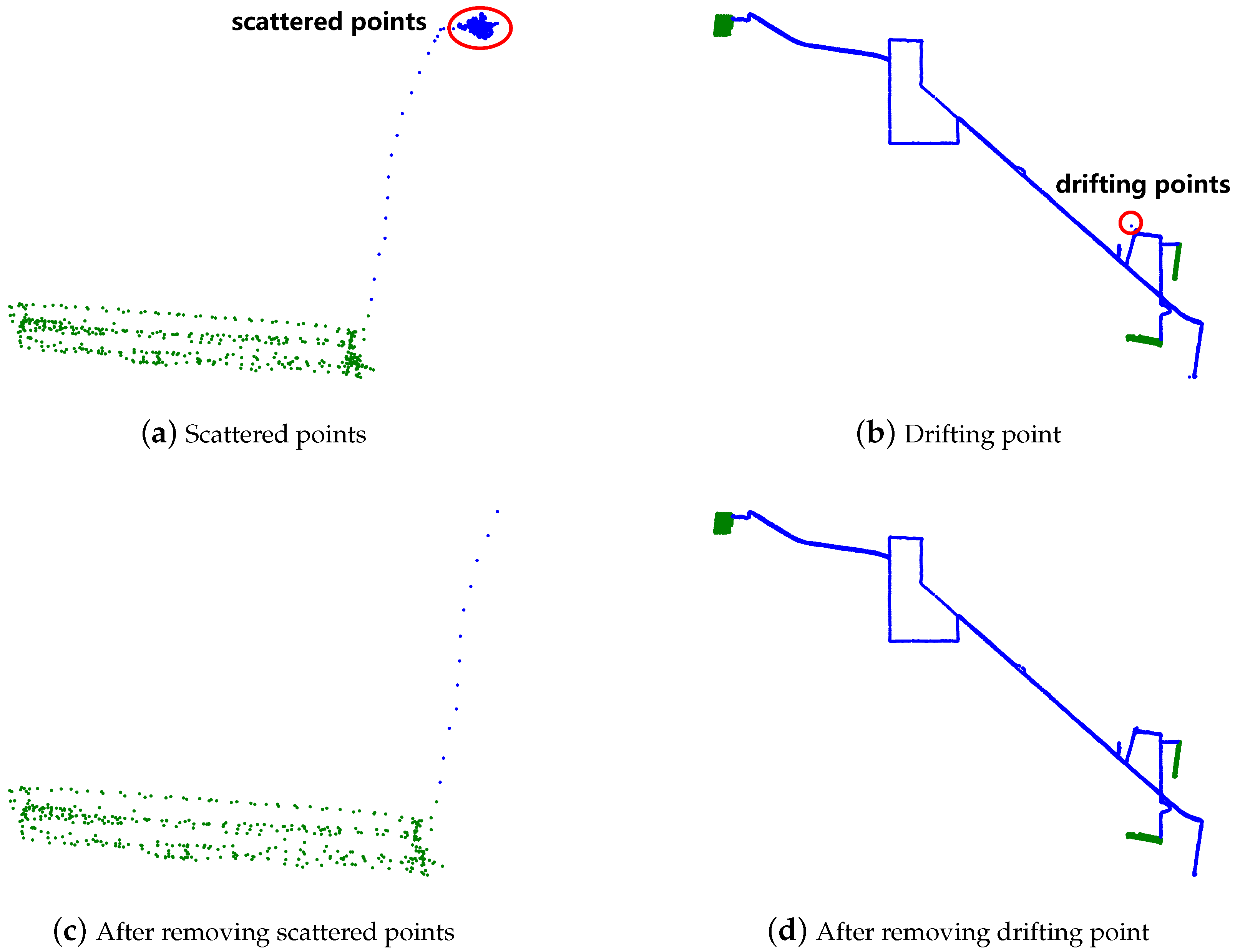
• Removing scattered points: When agricultural machinery is parked on the road or entering/exiting a garage, the GNSS receiver records many scattered road points with high density. These points are scattered within a small range around the actual position of agricultural machinery and need to be removed. Therefore, a rule-based cleaning method is proposed to effectively remove the scattered points and is formulated as follows:

  $$\Delta lo{n}_k=lo{n}_k-lo{n}_{k-1},\Delta la{t}_k=la{t}_k-la{t}_{k-1}$$

  (1)

  $$b={sin}^2\left(\frac{\Delta la{t}_k}{2}\right)+cos\left(la{t}_{k-1}\right)\times cos\left(la{t}_k\right)\times {sin}^2\left(\frac{\Delta lo{n}_k}{2}\right)$$

  (2)

  $$c=2\times arctan2(\sqrt{b},\sqrt{1-b}),R=6371000,\Delta d_k=R\times c$$

  (3)

$$dAverag{e}_k=\frac{1}{t}\sum _{i=k}^{k+t}\Delta d_i$$

(4)

$$\mathrm{if}dAverag{e}_k\le l,\mathrm{remove}\left(P_k\right)$$

(5)

where $\Delta d_k$ denotes the distance (m) feature of the kth point, $lo{n}_k$, $la{t}_k$, $\Delta lo{n}_k$, and $\Delta la{t}_k$ respectively denote the longitude, latitude, longitude variation, and latitude variation features of the kth point, R represents the average radius of the Earth (m), l denotes the threshold for determining whether to delete the scattered point, $dAverag{e}_k$ denotes the average value of distance variation from the point k to the point $k+t$, and remove($P_k$) is used to delete the scattered point $P_k$.

In this paper, the t is 20, which is recommended by Poteko et al. [18]. The t refers to the number of adjacent points, and it is used to calculate the average value of the distance variation of each t point(s). This average value is named the average distance feature $dAverag{e}_k$ of the current point $P_k$, which reflects the clustering tendency of trajectory segments. In addition, the l is set to 0.5. By comparing l with the $dAverag{e}_k$, it is determined whether $P_k$ is a scattered point.

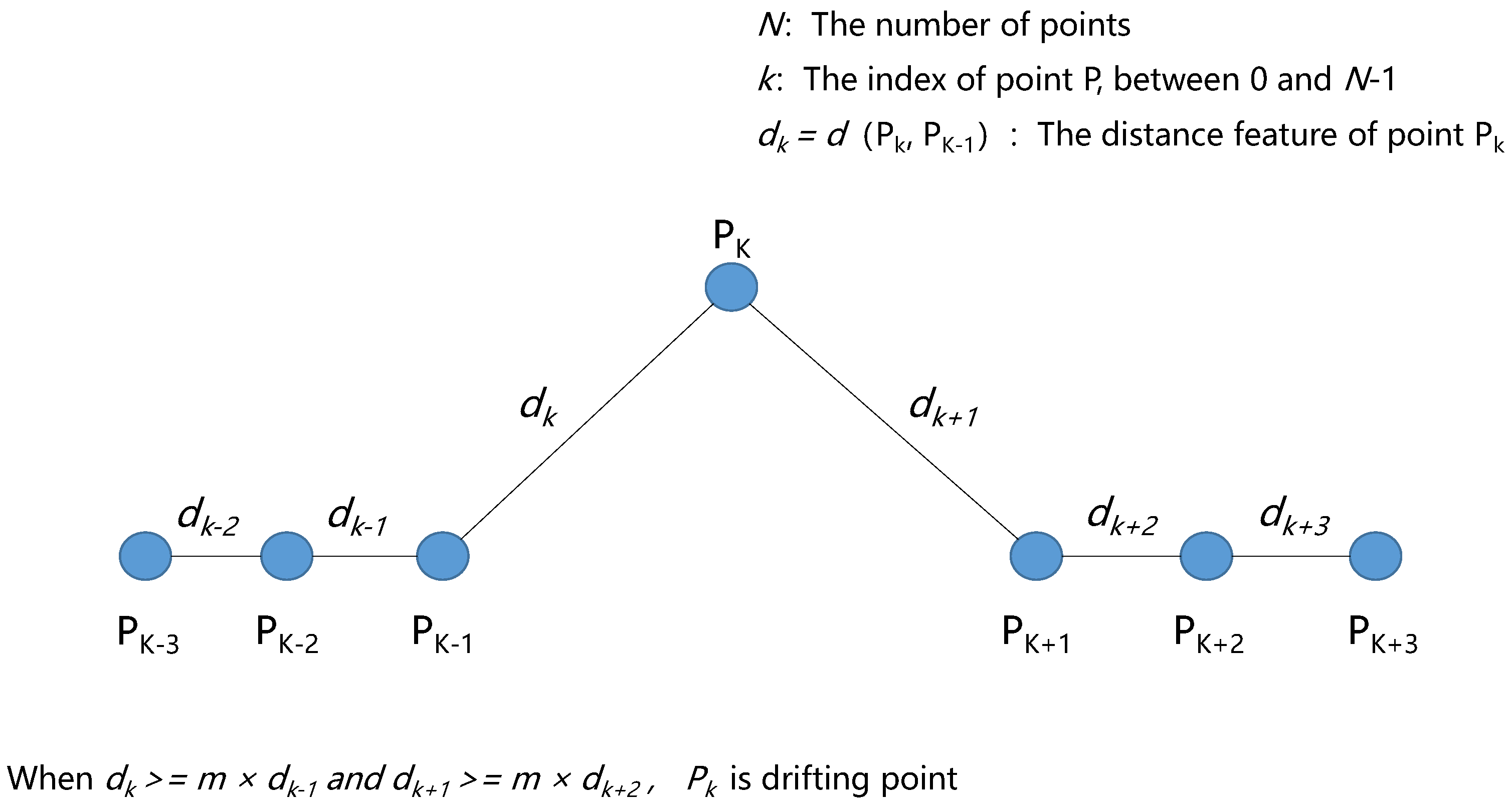
• Removing drifting points: When the distance features from a GNSS point to both its previous point and its next point are very large, the point is taken as a drifting point (see Figure 1). In this case, the drifting point is removed, its previous point becomes the ending point of the preceding trajectory segment, and its next point becomes the starting point of the subsequent trajectory segment.

Specifically, the method of removing drifting points is formulated as follows:

$$\left\{\begin{array}{c}\mathrm{d}\left(P_k,P_{k-1}\right)\ge m\times \mathrm{d}\left(P_{k+1},P_k\right), k=1, \mathrm{remove}\left(P_{k-1}\right).\\ \mathrm{d}\left(P_k,P_{k-1}\right)\ge m\times \mathrm{d}\left(P_{k-1},P_{k-2}\right)and\mathrm{d}\left(P_{k+1},P_k\right)\ge m\times \mathrm{d}\left(P_{k+2},P_{k+1}\right), 2\ge k\ge N-3, \mathrm{remove}\left(P_k\right).\\ \mathrm{d}\left(P_{k+1},P_k\right)\ge m\times \mathrm{d}\left(P_k,P_{k-1}\right), k=N-2, \mathrm{remove}\left(P_{k+1}\right).\end{array}\right.$$

(6)

where N denotes the point number of a given GNSS trajectory, k denotes the index between 0 and $N-1$ of a GNSS point, d($P_k$,$P_{k-1}$) is used to calculate the distance between the point $P_k$ and the point $P_{k-1}$, m denotes the threshold for determining whether to delete the drifting point, $P_k$ denotes the kth point, and remove($P_{k-1}$) is used to delete the drifting point $P_{k-1}$.

In this paper, the m is set to 6. Moreover, the drifting point is determined by utilizing the distance and the distance multiplied by m (see Figure 1).

As shown in Figure 2c,d, the scattered road points and the drifting points are removed by our proposed cleaning method, which suggests that our method is effective in removing the abnormal points.

In addition, some suggestions for the selection of the threshold l are as follows. When the l is significantly larger than 0.5 (e.g., 5 and 50), a large number of field points will be mistakenly deleted because the average distance features of field points are relatively small. Therefore, it is recommended not to set the l too large. Moreover, if the l is significantly smaller than 0.5 (e.g., 0.05 and 0.005), it will be difficult to identify scattered points.

Finally, the codes of our data-cleaning method are available at https://github.com/AgriMachineryBigData/Field-road_mode_mining (accessed on 5 March 2024), ensuring the comprehensive understanding of our proposed method.

3. Methodology

This section delivers the framework of our proposed ConvTEBiLSTM network (see Figure 3). The framework can be divided into two main modules: input feature construction and ConvTEBiLSTM network-based field-road classification. Firstly, statistical feature extraction and positional encoding consist of the input feature construction. In addition, in the ConvTEBiLSTM network-based field-road classification, there are four parts: Conv1d.5x for extracting local trajectory features, Transformer-Encoder for extracting global trajectory features, BiLSTM for fusing local and global trajectory features, and Linear Classifier for field-road mode identification.

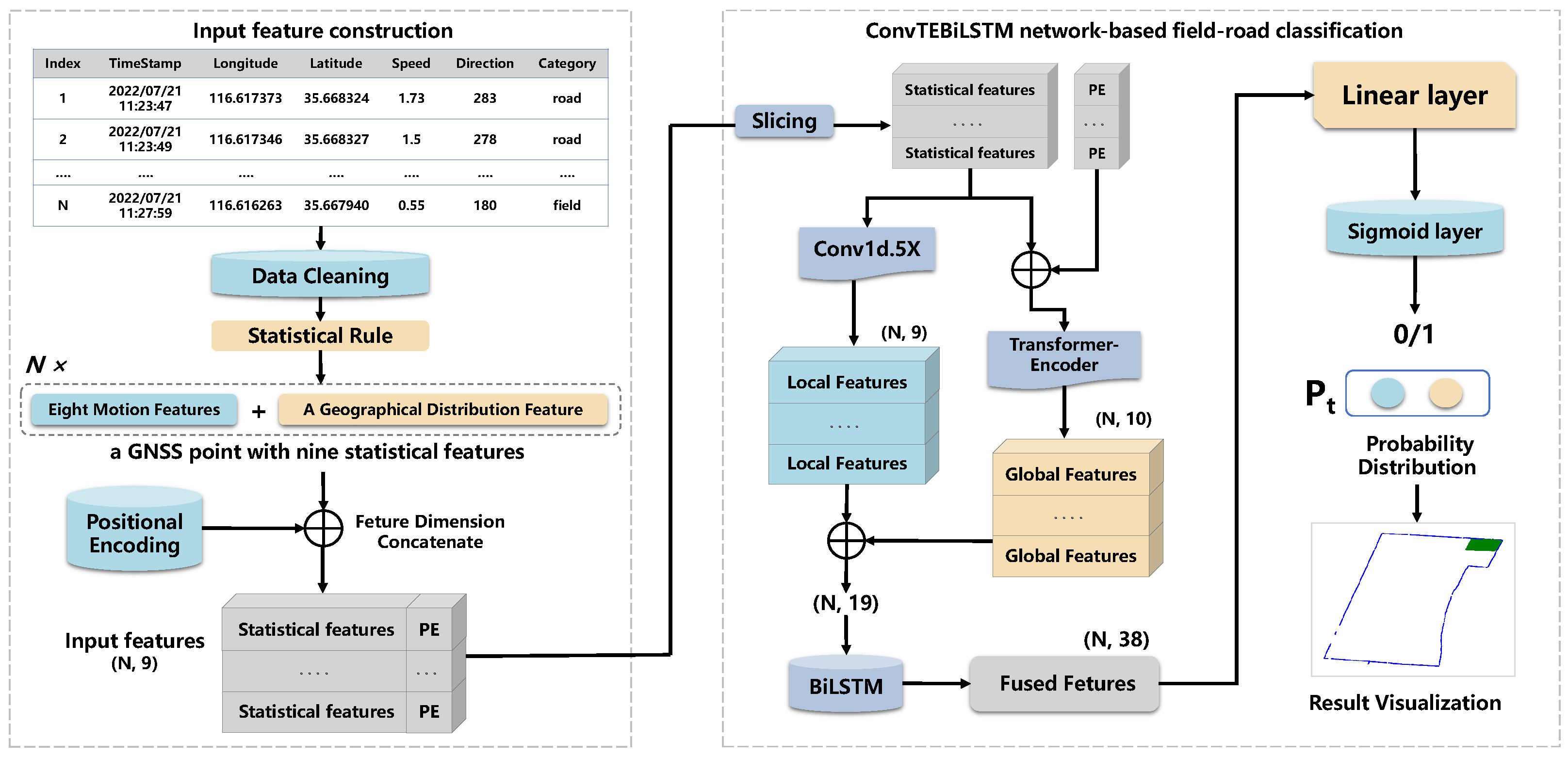
3.1. Input Feature Construction

3.1.1. Statistical Feature Extraction

Previous studies focus on using statistical features (i.e., the recorded parameters of GNSS trajectory data and derived parameters from the recorded parameters) as the input features of algorithms, but they primarily utilize the motion features (e.g., speed, direction, and acceleration) and ignore the geographical distribution features of GNSS points [18,19]. The geographical distribution features are useful for improving the overall performance of field-road mode classification because field points are usually more densely distributed than road points (see Figure 4).

Therefore, a statistical rule is designed to extract nine statistical features of each point from GNSS trajectory data: eight motion features and a geographical distribution feature. The motion features consist of speed, speed variation, acceleration, direction, direction variation, angular velocity, angular velocity variation, and distance. The geographical distribution feature represents the number of points within a square around the current point. Firstly, the extraction of eight motion features is defined as follows:

$$\Delta v_k=v_k-v_{k-1},a_k=\frac{\Delta v_k}{t_k-t_{k-1}}$$

(7)

$$\Delta di{r}_k=(di{r}_k-di{r}_{k-1}+{\theta }_1)mod{\theta }_1,{\theta }_1={360}^{\circ }$$

(8)

$${\omega }_k=\frac{\Delta di{r}_k}{t_k-t_{k-1}},\Delta {\omega }_k={\omega }_k-{\omega }_{k-1}$$

(9)

$$\Delta lo{n}_k=lo{n}_k-lo{n}_{k-1},\Delta la{t}_k=la{t}_k-la{t}_{k-1}$$

(10)

$$b={sin}^2\left(\frac{\Delta la{t}_k}{2}\right)+cos\left(la{t}_{k-1}\right)\times cos\left(la{t}_k\right)\times {sin}^2\left(\frac{\Delta lo{n}_k}{2}\right)$$

(11)

$$c=2\times arctan2(\sqrt{b},\sqrt{1-b}),R=6371000,\Delta d_k=R\times c$$

(12)

where $v_k$, $t_k$, $di{r}_k$, $\Delta v_k$, $a_k$, $\Delta di{r}_k$, ${\omega }_k$, $\Delta {\omega }_k$, and $\Delta d_k$ respectively denote the speed, timestamp, direction, speed variation ($m/s$), acceleration ($m/s^2$), direction variation (°), angular velocity (°$/s$), angular velocity variation (°$/s$), and distance (m) features of the kth point; $lo{n}_k$, $la{t}_k$, $\Delta lo{n}_k$, and $\Delta la{t}_k$ respectively denote the longitude, latitude, longitude variation, and latitude variation features of the kth point; R represents the average radius of the Earth (m); and mod denotes the modulo operation.

Subsequently, the geographical distribution features are calculated by Algorithm 1:

Algorithm 1 Calculate Geographical Distribution Features

1: function ConvertToPlaneCoordinates(lon_WGS, lat_WGS) 2:     in_proj ← CRS(“EPSG:4326”)                     ▹ WGS84 3:     out_proj ← CRS(“EPSG:32633”)             ▹ UTM Zone 33N 4:     transformer ← Transformer.from_crs(in_proj, out_proj, always_xy=True) 5:     lon_UTM, lat_UTM ← transformer.transform(lon_WGS, lat_WGS) 6:     return lon_UTM, lat_UTM 7: end function 8: function GeoDistributionFeatures(current_point, gnss_data, square_width) 9:     square_left ← current_point[’lon_UTM’] - square_width / 2 10:   square_right ← current_point[’lon_UTM’] + square_width / 2 11:   square_bottom ← current_point[’lat_UTM’] - square_width / 2 12:   square_top ← current_point[’lat_UTM’] + square_width / 2 13:   lon_UTM, lat_UTM ← ConvertToPlaneCoordinates( 14:           [point[’lon_WGS’] for point in gnss_data], 15:           [point[’lat_WGS’] for point in gnss_data]) 16:   count ← np.sum((lon_UTM ≥ square_left) & (lon_UTM ≤ square_right) & (lat_UTM ≥ square_bottom) & (lat_UTM ≤ square_top)) 17:   return count 18: end function

where $lon\_WGS$ and $lat\_WGS$ denote the geographical coordinates (WGS84), $lon\_UTM$ and $lat\_UTM$ denote the plane coordinates (UTM), ConvertToPlaneCoordinates function is used to convert geographical coordinates to plane coordinates, $gnss\_data$ denotes all points of a given trajectory, $square\_width$ denotes the width of the square region around the point $current\_point$, and GeoDistributionFeatures function is used to calculate the number of points within the specified square region.

In this paper, the $square\_width$ is 10. The average value of the geographical distribution features of the field points on each GNSS trajectory is larger than the road points because of the lower driving speed of agricultural machinery and the closer distance between consecutive GNSS points (see Figure 5).

3.1.2. Positional Encoding

When dealing with temporal-related tasks, the order of each input feature vector is essential for the Transformer-Encoder network to capture the temporal dependencies among feature vectors [26]. Therefore, by using positional encoding, the positional information is introduced to each point in a given GNSS trajectory. The positional encoding is defined as follows:

$$\mathrm{PE}\left(pos\right)=sin\left(pos\right), 0\le pos\le N-1$$

(13)

where $\mathrm{PE}\left(pos\right)$ is used to obtain the positional encoding for the posth point, and N denotes the number of points in a given GNSS trajectory.

After the statistical feature extraction and positional encoding processes, each GNSS point has nine statistical features and a positional encoding and then is used as the final input feature vector of neural networks.

3.2. ConvTEBiLSTM Network-Based Field-Road Classification

In this paper, we set the output feature dimension of each neural network module to be the same as the input feature dimension (see Figure 3) rather than being a multiple of it to improve training and inference efficiency, minimize redundant latent features, enhance model interpretability, and mitigate the risk of overfitting.

3.2.1. Conv1d.5x for Extracting Local Trajectory Features

The Conv1d.5x network consists of a 1D convolution kernel ($input\_channel$ = 9, $output\_channel=9$, $kernel\_size=5$, $stride=1$, $padding=2$) and a Relu activation function (see Figure 3). The 1D convolution kernel is used to extract nine local trajectory features of a point from five temporal neighboring input feature vectors. Specifically, the $kernel\_size$, $stride$, and $padding$ of the Conv1d.5x network are respectively set to 5, 1, and 2 to preserve the temporal structure of the input features during the convolution operation. Firstly, the $kernel\_size$ is set to 5, which indicates that each convolution operation considers continuous 5 GNSS points from a given trajectory, to capture local latent features. Secondly, the $stride$ is set to 1, meaning that the convolution operation computes at every position of a given trajectory to ensure comprehensive feature extraction across the entire trajectory. Finally, the $padding$ is set to 2 for padding the 2 zero values at both ends of the input trajectory, which ensures that convolution operations are correctly computed at the edges while maintaining the same size for the output sequence as the input sequence. The Conv1d.5x network is formulated as follows:

$$Y_i^{\left(c\right)}=\sum _{j=0}^{k-1}{X}_{i+j}^{\left(c\right)}·K_j^{\left(c\right)}$$

(14)

where k denotes the size of the convolution kernel, c denotes the channel index of the input feature vector, j denotes the offset position of the convolution kernel, i denotes the position in the output sequence, $K_j^{\left(c\right)}$ denotes the jth weight of the convolution kernel in the cth channel, $X_{i+j}^{\left(c\right)}$ denotes the $i+j$th vector in the input sequence of the cth channel, and $Y_i^{\left(c\right)}$ denotes the ith element in the output sequence of the cth channel.

3.2.2. Transformer-Encoder for Extracting Global Trajectory Features

Most previous studies have proved that the Transformer neural network with encoder and decoder modules [26] is effective in extracting global features from original data by using the self-attention mechanism [27]. In this paper, the Transformer-Encoder ($d\_model=10$, $nhead=10$, $activation=relu$, $dim\_feedforward=256$, $num\_layers=4$) is used to extract 10 global trajectory features of a point from all input feature vectors. The input sequence is denoted as X= $\left[x_1,x_2,\dots ,x_T\right]$, where T is the number of input feature vectors, and each $x_i$ is a vector containing ten input features. The Transformer-Encoder mainly consists of self-attention layers and feed-forward neural networks. The self-attention layer of the Transformer-Encoder is formulated as follows:

$$Q_i^{\left(h\right)}=x_i·W_{Qi}^{\left(h\right)},K_j^{\left(h\right)}=x_j·W_{Ki}^{\left(h\right)},V_j^{\left(h\right)}=x_j·W_{Vi}^{\left(h\right)}$$

(15)

where i and j denote the position indices in the input sequence X, h represents the index of the attention head in the self-attention mechanism, $x_i$ and $x_j$ are the feature vectors of the input sequence, $Q_i^{\left(h\right)}$ represents the query vector at position i in attention head h, $K_j^{\left(h\right)}$ represents the key vector at position j in attention head h, $V_j^{\left(h\right)}$ represents the value vector at position j in attention head h, and $W_{Qi}^{\left(h\right)}$, $W_{Ki}^{\left(h\right)}$, and $W_{Vi}^{\left(h\right)}$ are learned weight matrices.

$$\mathrm{Attention}(Q_i^{\left(h\right)},K_j^{\left(h\right)},V_j^{\left(h\right)})=\frac{exp(Q_i^{\left(h\right)}·K_j^{\left(h\right)}/\sqrt{d_{\mathrm{head}}})}{{\sum }_{j=1}^{T}exp(Q_i^{\left(h\right)}·K_j^{\left(h\right)}/\sqrt{d_{\mathrm{head}}})}·V_j^{\left(h\right)}$$

(16)

where Attention($Q_i^{\left(h\right)}$,$K_j^{\left(h\right)}$,$V_j^{\left(h\right)}$) is used to compute the attention scores for each position in the input sequence by using a scaled dot-product attention formula, determining the importance of different positions for a given position i in the self-attention mechanism, $Q_i^{\left(h\right)}·K_j^{\left(h\right)}$ calculates the dot product between the query $Q_i^{\left(h\right)}$ and key $K_j^{\left(h\right)}$ vectors for positions i and j:

$$\mathrm{MultiHead}\left(X\right)=\mathrm{Concat}(\mathrm{Attention}(Q_i^{\left(h\right)},K_j^{\left(h\right)},V_j^{\left(h\right)})\forall h)·W_O$$

(17)

where MultiHead(X) is multi-head attention and is used to apply the self-attention mechanism on each attention head h and obtain the output sequence, Concat function is used to concatenate the outputs from each head along a certain dimension, and $W_O$ is the weight matrix and is used to linearly transform the concatenated output from the multi-head attention for producing the final output.

The feed-forward neural network of the Transformer-Encoder is formulated as follows:

$$\mathrm{FFN}\left(X\right)=\mathrm{ReLU}(X·W_1+b_1)·W_2+b_2$$

(18)

where FFN(X) is used to capture complex and non-linear relationships in the input sequence, Relu function applies an element-wise rectification for setting all negative values to zero, $W_1$ is the weight matrix for the first linear transformation in the feed-forward network, $W_2$ is the weight matrix for the second linear transformation, and $b_1$ and $b_2$ are bias vectors added to the respective linear transformations.

Finally, the layer normalization and residual connection are applied to obtain the final output:

$$\mathrm{Output}=\mathrm{LayerNorm}\left(\mathrm{FFN}\right(\mathrm{MultiHead}\left(X\right))+X)$$

(19)

where LayerNorm function is a normalization technique that standardizes the output of a neural network layer, FFN(MultiHead(X) + X) performs a residual connection operation for adding the output of the feed-forward network to the input sequence, and Output is the final output with global trajectory features of the Transformer-encoder.

3.2.3. BiLSTM for Fusing Local and Global Trajectory Features

Firstly, the local features extracted by Conv1d.5x and the global features extracted by the Transformer-Encoder are concatenated in the feature dimension. Subsequently, the concatenated features are fed into a BiLSTM [28] ($input\_size$ = 19, $hidden\_size$ =19, and $number\_layers$=2) for fusing the local and global trajectory features. The BiLSTM contains two LSTM modules, and the LSTM module is formulated as follows:

$$h_i=LSTM(x_i,h_{i-1})$$

(20)

where $x_i$ is the local and global feature vector of the ith point, and $h_i$ is the hidden state.

$$\overrightarrow{h_i}=\mathrm{LSTM}(x_i,\overrightarrow{h_{i-1}}),\overleftarrow{h_i}=LSTM(x_i,\overleftarrow{h_{i+1}}),h_i=[\overrightarrow{h_i},\overleftarrow{h_i}]$$

(21)

where $\overrightarrow{h_i}$ can capture the temporal relationships from past points, and $\overleftarrow{h_i}$ can learn the temporal dependencies from future points.

By using a trajectory and its reverse, the BiLSTM learns $h_t$, which combines the past temporal with future temporal information and fuses the local and global trajectory features.

3.2.4. Linear Classifier for Field-Road Mode Identification

Based on $h_i$, the ith point is classified by a fully connected layer ($in\_features$ = 38, and $ou\_features$ = 2). Then, its predicted probability distribution $p_i$ on “field” and “road” categories is obtained by using a sigmoid activation function [29]. The sigmoid activation function is formulated as follows:

$$f\left(x\right)=\frac{1}{1+e^{-x}}$$

(22)

where e refers to the mathematical constant known as Euler’s number, which is approximately equal to 2.71828, and the x represents the input to the sigmoid function.

4. Experiments

4.1. Experimental Settings

4.1.1. Comparison Methods

To evaluate the classification performance of our method, five famous temporal-related networks are used as the baselines: 1D Convolutional Neural Network (1D-CNN), Transformer-Encoder Neural Network (TE), Bidirectional Long Short-Term Memory Neural Network (BiLSTM), Convolutional Bidirectional Long Short-Term Memory Neural Network (ConvBiLSTM), and Transformer+BiLSTM Neural Network (TE-BiLSTM). The operation environment used for training and testing has an Intel Xeon Processor (Icelake) CPU and three NVIDIA A100 (40G) GPUs, and all neural networks are performed in Python language on Ubuntu 20.04 LTS (GNU/Linux 5.4.0-139-generic x86_64) using PyTorch API [30].

4.1.2. Model Training Process

In this paper, there are 200 epochs for model training. In addition, there is a field-road class imbalance problem (i.e., the number of field points is much higher than road points) on the Harvester. In order to tackle the imbalance problem, the focal loss (FC) [31] is used in this paper. The focal loss can decrease the weight of easily distinguishable points by a dynamic scaling factor so that more attention is given to those indistinguishable points during the model training [21]. The focal loss is formulated as follows:

$$FC=-\alpha {\left(1-\widetilde{p_t}\right)}^{\gamma }log\left(\widetilde{p_t}\right)$$

(23)

where $\widetilde{p_t}$ refers to the probability of the $\mathit{t}$-th point with the predicted category (i.e., field or road), and $\alpha$ and $\gamma$ are pre-defined parameters. The $\alpha$ is used to deal with the field-road class imbalance, and $\gamma$ is utilized to reduce the contribution of easily predicted points to the final loss. The $\alpha$ is set to 0.25, and $\gamma$ is set to 2, which are recommended by Lin et al. [31].

In addition, the popular AdamW optimizer [32] is used to optimize our models and enhance the generalization ability of the models by refining the weight decay mechanism. In this paper, the weight decay is set to 0.00001, and the learning rate is set to 0.0001 in the AdamW optimizer, which are recommended by Loshchilov et al. [33]. Finally, considering the overfitting, arising when a machine learning model performs well on the training dataset but poorly on the unseen testing dataset, we utilize the early stopping technique to mitigate this overfitting. Early stopping involves monitoring the performance of the model on a validation dataset during training and stopping the training process when the performance on the validation dataset stops improving or starts to degrade. This prevents the model from overfitting to the training data, thereby improving its generalization ability.

4.1.3. Performance Metrics

Firstly, precision (P), recall (R), F1-score (F1), and accuracy (Acc) are utilized for performance evaluation. The four metrics are defined by using the confusion matrix, including true positive (TP), true negative (TN), false positive (FP), and false negative (FN) [34]. For instance, the “field” category is regarded as the “positive” category, and the “road” category is regarded as the “negative” category. Therefore, TP represents the field points correctly classified as “field”, TN represents the road points correctly classified as “road”, FP represents the road points incorrectly classified as “field”, and FN represents the field points incorrectly classified as “road”. Furthermore, for “positive” category, P reflects the ability of the neural network to correctly identify the GNSS points with “positive” category in the predicted data, R shows the ability of the neural network to detect the GNSS points with “positive” category in the ground-truth data, and F1 is a harmonic means of the P and R. Acc is the ratio of the number of correctly predicted points to the total number of input points. In addition, model size and inference time are utilized for the full evaluation. Specifically, the inference time refers to the average time it takes for the model to predict all test trajectories, and the model size refers to the amount of space occupied by the model on storage devices:

$$P=\frac{TP}{TP+FP}$$

(24)

$$R=\frac{TP}{TP+FN}$$

(25)

$$F1=2\times \frac{P\times R}{P+R}$$

(26)

$$Acc=\frac{TP+TN}{TP+TN+FP+FN}$$

(27)

4.1.4. Model Testing

K-fold cross-validation [35] is used for evaluating the classification performance of various methods. In this paper, K = 10 is taken, which is recommended by Stone et al. [36], Westerhuis et al. [37] and Neunhoeffer et al. [38], allowing to fully test the model performance. Firstly, the Harvester dataset is randomly divided into K equivalent parts (${\mathit{C}}_1$, ${\mathit{C}}_2$,…, ${\mathit{C}}_K$) with $\mathit{n}$ trajectories in each part. Then, the ${\mathit{C}}_i$ data are utilized as the validation dataset ($\mathit{i}$∈ (1, 2, …, $\mathit{k}$)), and the remaining parts are used as the training dataset for K iterations until the cross-validation is completed.

4.2. Results and Discussion

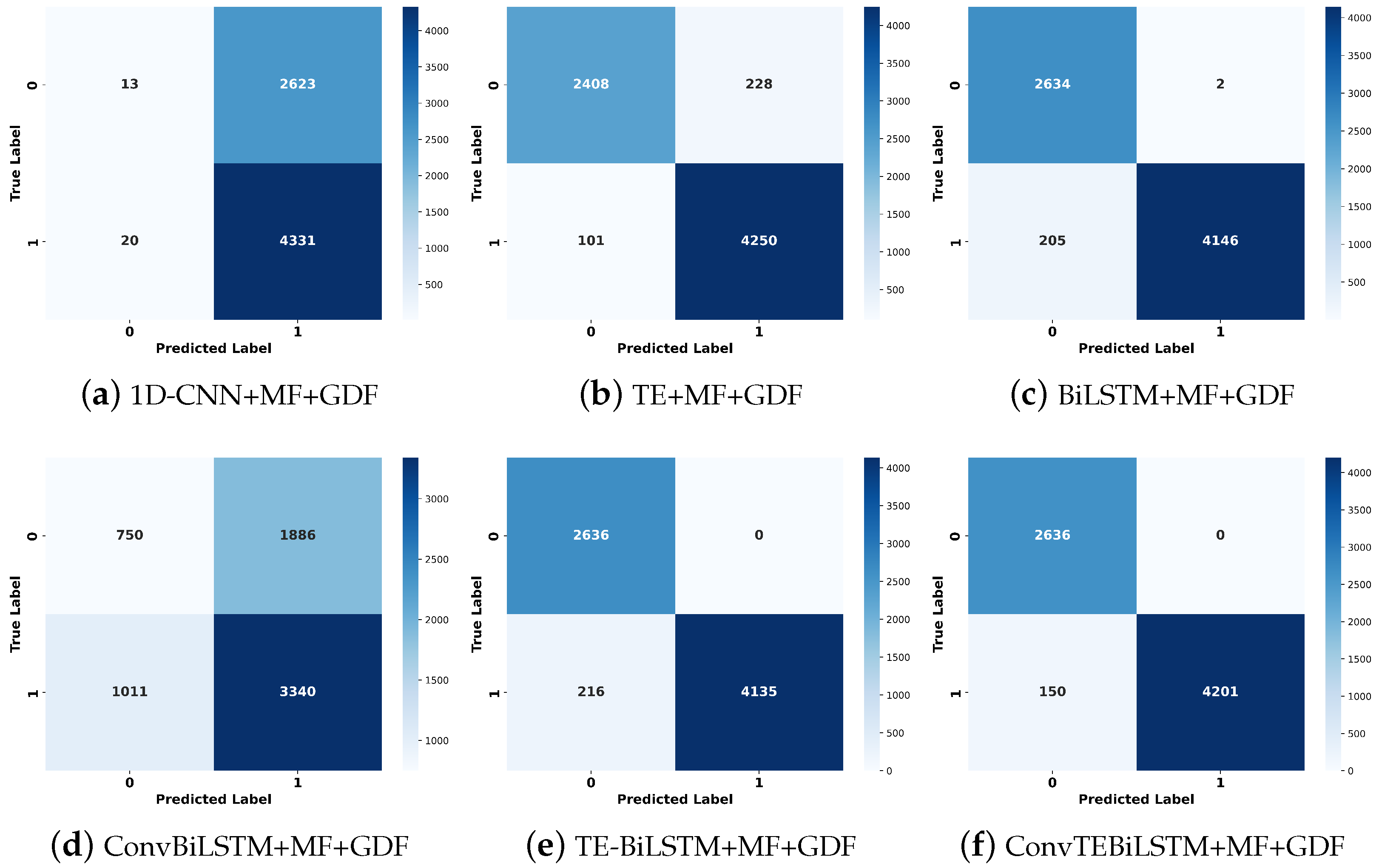
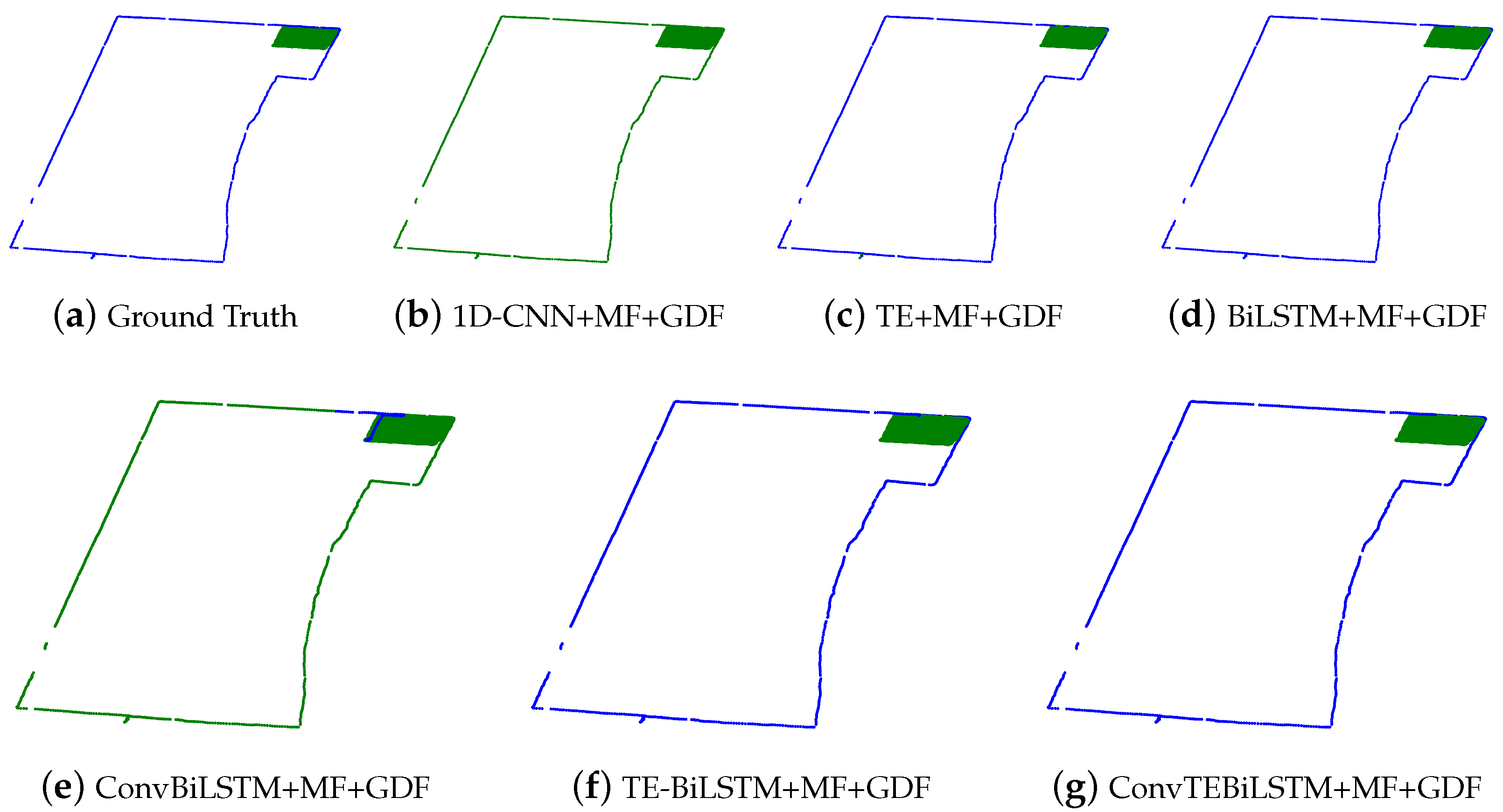
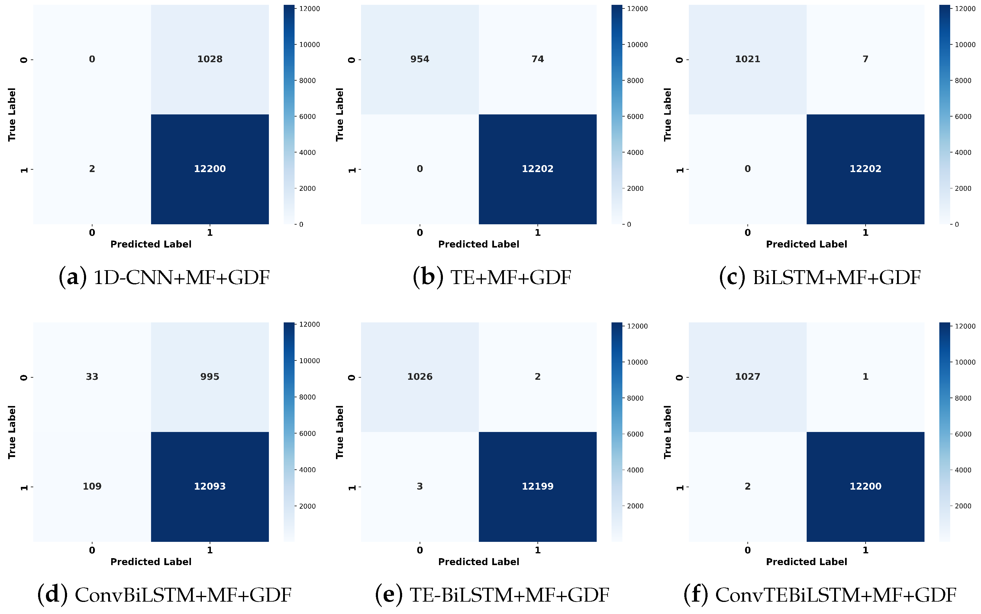
4.2.1. Method Comparisons and Analysis

Table 2. The overall classification performances of the six methods on the Harvester dataset.

Method	P	R	F1	Acc	Model Size/kb	Inference Time/s
1D-CNN+MF+GDF	45.11	49.97	45.88	85.09	20.6	0.828824
TE+MF+GDF	91.07	82.55	85.34	94.29	112	0.798763
ConvBiLSTM+MF+GDF	46.91	50.33	47.80	84.13	20.7	0.925290
TE-BiLSTM+MF+GDF	94.01	91.52	91.79	96.59	132	0.968573
BiLSTM+MF+GDF	93.38	91.17	91.14	96.32	17.7	0.981394
ConvTEBiLSTM+MF+GDF	95.60	91.60	92.74	97.38	179	0.998893

MF: motion features; GDF: geographical distribution feature; P: Precision; R: Recall; F1: F1-score; Acc: Accuracy.

shows the overall classification performance of our proposed method and the baselines. Although the model size and inference time are not the smallest and fastest of all methods, our method (ConvTEBiLSTM+MF+GDF) achieves superior performance in accurately classifying field-road modes. Specifically, compared with the baselines, our method (ConvTEBiLSTM+MF+GDF) achieves the best accuracy of 97.38% and the highest F1-score of 92.74%. In addition, the results demonstrate that our method (ConvTEBiLSTM+MF+GDF) achieves a 0.79% accuracy increase and a 0.95% F1-score improvement over the best method (TE-BiLSTM+MF+GDF). The above results suggest that our method (ConvTEBiLSTM+MF+GDF) is effective in differentiating field points from road points and viable for real-world applications. The different performance results of the six field-road mode classification methods can be attributed to the feature extraction abilities of the used neural networks and the strategy of feature fusion. Specifically, the 1D-CNN+MF+GDF method uses the 1D-CNN to extract the local trajectory features from temporal neighboring points in a GNSS trajectory but ignores the feature fusion. The TE+MF+GDF method uses the TE to extract the global trajectory features from all GNSS points and also ignores the feature fusion. The BiLSTM+MF+GDF method captures the past and future temporal relationships between the current point and its last-next points but ignores the local and global trajectory features. In addition, the ConvBiLSTM+MF+GDF and TE-BiLSTM+MF+GDF methods consider feature fusion but ignore either global trajectory features or local trajectory features.

Different from the baselines, our method (ConvBiLSTM+MF+GDF) extracts and fuses the local and global trajectory features by combining multiple neural networks. Specifically, we use the 1D-CNN and TE to extract the local and global trajectory features, respectively. Subsequently, the global trajectory features extracted by TE and the local trajectory features extracted by 1D-CNN are concatenated in the feature dimension. Finally, the concatenated features are fed into the BiLSTM and are effectively fused by the BiLSTM. The success of our ConvTEBiLSTM network highlights the importance of combining different neural networks for field-road mode classification to take advantage of their strengths.

Figure 6 and Figure 7 show the classification results and confusion matrices of the six methods in a a harvester trajectory with multiple fields. In addition, Figure 8 and Figure 9 show the classification results and confusion matrices of the six methods in a trajectory with a field. It can be intuitively seen that compared with two ground-truth harvester trajectories, our ConvTEBiLSTM network performs the best in terms of classification performance. For instance, the confusion matrix (see Figure 7) shows that our method (ConvTEBiLSTM+MF+GDF) achieves the largest number of correctly classified points and outperforms the baseline (TE-BiLSTM+MF+GDF) by 66 points in the Harvester trajectory with multiple fields, significantly alleviating incorrectly classified points. However, compared with the harvester trajectory with multiple fields, the classification performance of our method (ConvTEBiLSTM+MF+GDF) on the harvester trajectory with a field is much better. This is because there are a few field points with low density similar to the road points on the harvester trajectory with multiple fields. This suggests that our method (ConvTEBiLSTM+MF+GDF) is more effective in the GNSS trajectory with high-density fields.

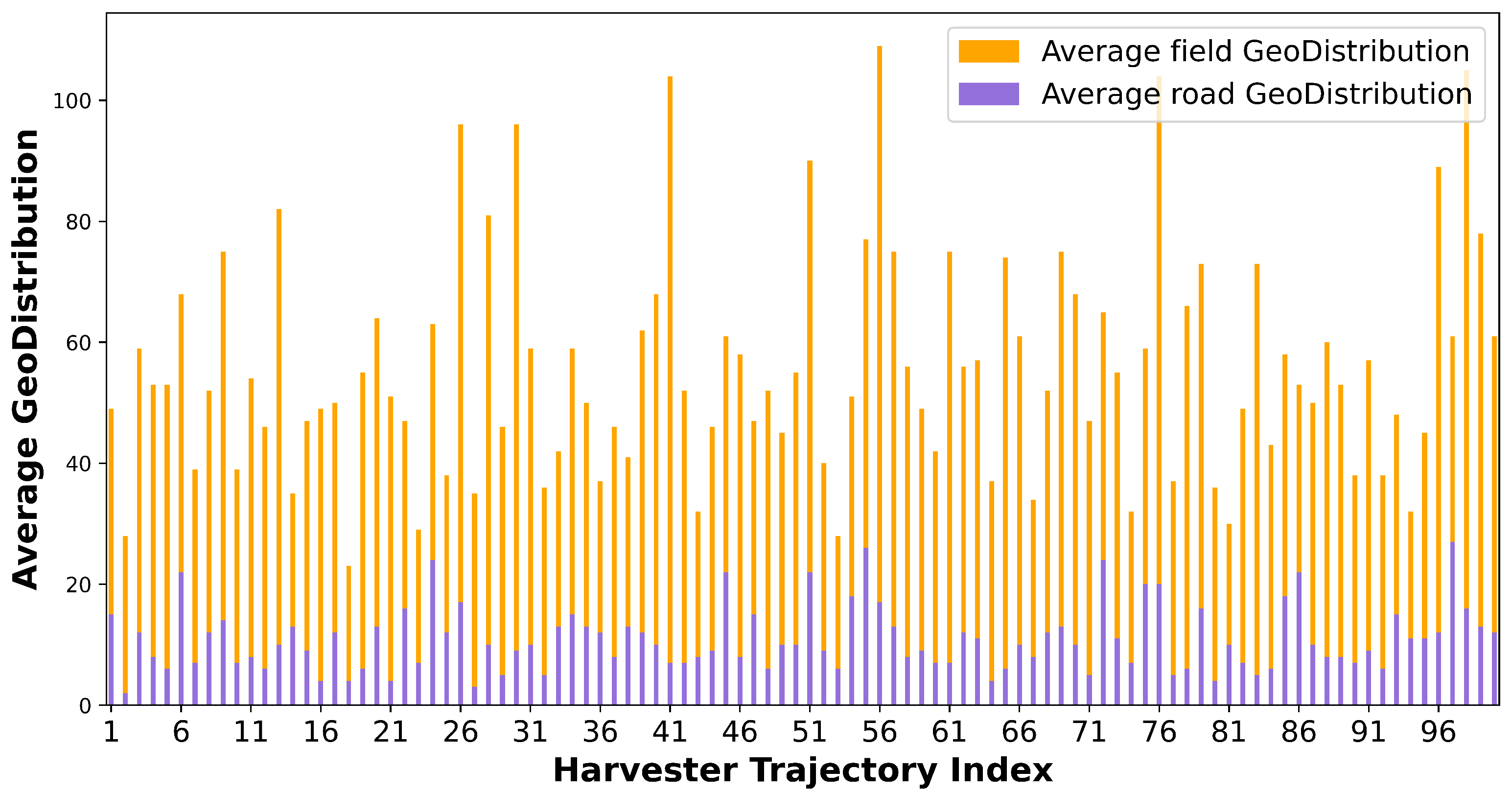
4.2.2. Effective of Geographical Distribution Feature

To investigate the impact of the geographical distribution feature (GDF), ablation studies are performed, and the results are shown in

Table 3. The overall classification performance results of the four methods on the Harvester dataset.

Method	P	R	F1	Acc
BiLSTM+MF	83.45	72.35	72.74	88.60
BiLSTM+MF+GDF	93.38	91.17	91.14	96.32
ConvTEBiLSTM+MF	51.79	52.23	49.40	84.41
ConvTEBiLSTM+MF+GDF	95.60	91.60	92.74	97.38

MF: motion features; GDF: geographical distribution feature; P: Precision; R: Recall; F1: F1-score; Acc: Accuracy.

. The results show that the overall performances of the two networks (i.e., BiLSTM and ConvTEBiLSTM) increase greatly by adding GDF to motion features (MF) on the Harvester. For instance, after adding the GDF to MF, the F1-score and accuracy of the ConvTEBiLSTM network respectively increase by 43.34% and 12.97%, and this suggests that the geographical distribution features are greatly useful to enhance the overall classification performance of neural networks.

Figure 10 shows visual results of a harvester trajectory, and Figure 11 shows the confusion matrix corresponding to the trajectory. The visual results suggest that compared with ConvTEBiLSTM+MF, ConvTEBiLSTM+MF+GDF significantly alleviates incorrectly classified points.

5. Conclusions

In this paper, a ConvTEBiLSTM network fusing local and global trajectory features is proposed to improve the accuracy of field-road mode classification. Firstly, a statistical rule is designed to extract eight motion features and a geographical distribution feature from the original trajectory data to enrich the feature representation of each point. Our method combines multiple neural networks to extract and fuse the local and global trajectory features for field-road classification. Experimental results demonstrate that the ConvTEBiLSTM network-based method respectively achieves the best accuracy and the highest F1-score of 97.38% and 92.74% on the Harvester dataset, outperforming the baselines. This suggests that fusing the local and global trajectory features is useful for improving the overall performance of field-road classification. By utilizing the accurate classification results, the field boundaries can be determined accurately, thereby effectively estimating the field area. This has important implications for agricultural production planning, land use planning, and the formulation of agricultural subsidy policies.

In the future, considering the potential for the shared bias of 10-fold cross-validation to exaggerate the model’s predictive performance, we will utilize more advanced strategies (e.g., stratified K-fold cross-validation, and repeated cross-validation) to further mitigate the impact of shared bias for achieving more effective classification performance evaluation. In addition, considering the suboptimality of the current threshold selection, in the future, we will conduct further research on threshold selection (e.g., l, t, and m) on our Harvester dataset and apply this method to other public trajectory datasets. Finally, we plan to design a robust field-road classification method that can effectively handle the problem of difficulty in improving the identification accuracy of fields with low density.

References

1. Keller, T.; Lamandé, M.; Peth, S.; Berli, M.; Delenne, J.Y.; Baumgarten, W.; Rabbel, W.; Radjai, F.; Rajchenbach, J.; Selvadurai, A.; et al. An interdisciplinary approach towards improved understanding of soil deformation during compaction. Soil Tillage Res. 2013, 128, 61–80. [Google Scholar] [CrossRef]
2. Damanauskas, V.; Janulevicius, A.; Pupinis, G. Influence of extra weight and tire pressure on fuel consumption at normal tractor slippage. J. Agric. Sci. 2015, 7, 55–67. [Google Scholar] [CrossRef]
3. Zhang, F.Z.; Liu, R.H.; Ni, Y.D.; Wang, Y. Dynamic positioning accuracy test and analysis of Beidou satellite navigation system. GNSS World China 2018, 3, 43–48. [Google Scholar]
4. Li, D.; Liu, X.; Zhou, K.; Sun, R.; Wang, C.; Zhai, W.; Wu, C. Discovering spatiotemporal characteristics of the trans-regional harvesting operation using big data of GNSS trajectories in China. Comput. Electron. Agric. 2023, 211, 108003. [Google Scholar] [CrossRef]
5. Zhai, W.; Mo, G.; Xiao, Y.; Xiong, X.; Wu, C.; Zhang, X.; Xu, Z.; Pan, J. GAN-BiLSTM network for field-road classification on imbalanced GNSS recordings. Comput. Electron. Agric. 2024, 216, 108457. [Google Scholar] [CrossRef]
6. Bochtis, D.D.; Sørensen, C.G.; Busato, P. Advances in agricultural machinery management: A review. Biosyst. Eng. 2014, 126, 69–81. [Google Scholar] [CrossRef]
7. Sopegno, A.; Calvo, A.; Berruto, R.; Busato, P.; Bocthis, D. A web mobile application for agricultural machinery cost analysis. Comput. Electron. Agric. 2016, 130, 158–168. [Google Scholar] [CrossRef]
8. Molari, G.; Mattetti, M.; Lenzini, N.; Fiorati, S. An updated methodology to analyse the idling of agricultural tractors. Biosyst. Eng. 2019, 187, 160–170. [Google Scholar] [CrossRef]
9. Pagare, V.; Nandi, S.; Khare, D. Appraisal of Optimum Economic Life for Farm Tractor: A Case Study. Econ. Aff. 2019, 64, 117–124. [Google Scholar] [CrossRef]
10. Li, X.; Hao, F. Research on Agricultural Machinery Behavior Recognition and Application System Based on Satellite Remote Sensing Image. Master’s Thesis, Qilu University of Technology, Jinan, China, 2023. [Google Scholar]
11. Wu, C.; Li, D.; Zhang, X.; Pan, J.; Quan, L.; Yang, L.; Yang, W.; Ma, Q.; Su, C.; Zhai, W. Application note: China’s agricultural machinery operation big data system. Comput. Electron. Agric. 2023, 205, 107594. [Google Scholar] [CrossRef]
12. Song, X.P.; Potapov, P.V.; Krylov, A.; King, L.; Di Bella, C.M.; Hudson, A.; Khan, A.; Adusei, B.; Stehman, S.V.; Hansen, M.C. National-scale soybean mapping and area estimation in the United States using medium resolution satellite imagery and field survey. Remote Sens. Environ. 2017, 190, 383–395. [Google Scholar] [CrossRef]
13. Song, X.; Wu, F.; Lu, X.; Yang, T.; Ju, C.; Sun, C.; Liu, T. The classification of farming progress in rice–wheat rotation fields based on UAV RGB images and the regional mean model. Agriculture 2022, 12, 124. [Google Scholar] [CrossRef]
14. Bereżnicka, J.; Wicki, L. Do operating subsidies increase labour productivity in Polish farms? Stud. Agric. Econ. 2021, 123. [Google Scholar]
15. Xiao, Y.; Mo, G.; Xiong, X.; Pan, J.; Wu, C.; Zhai, W. DR-XGBoost: An XGBoost model for field-road segmentation based on dual feature extraction and recursive feature elimination. Int. J. Agric. Biol. Eng. 2023, 16, 169–179. [Google Scholar] [CrossRef]
16. Chen, Y.; Zhang, X.; Wu, C.; Li, G. Field-road trajectory segmentation for agricultural machinery based on direction distribution. Comput. Electron. Agric. 2021, 186, 106180. [Google Scholar] [CrossRef]
17. Ester, M.; Kriegel, H.P.; Sander, J.; Xu, X. A density-based algorithm for discovering clusters in large spatial databases with noise. In Proceedings of the KDD’96: Proceedings of the Second International Conference on Knowledge Discovery and Data Mining, Portland OR, USA, 2–4 August 1996; Volume 96, pp. 226–231. [Google Scholar]
18. Poteko, J.; Eder, D.; Noack, P.O. Identifying operation modes of agricultural vehicles based on GNSS measurements. Comput. Electron. Agric. 2021, 185, 106105. [Google Scholar] [CrossRef]
19. Chen, Y.; Li, G.; Zhang, X.; Jia, J.; Zhou, K.; Wu, C. Identifying field and road modes of agricultural Machinery based on GNSS Recordings: A graph convolutional neural network approach. Comput. Electron. Agric. 2022, 198, 107082. [Google Scholar] [CrossRef]
20. Zitnik, M.; Agrawal, M.; Leskovec, J. Modeling polypharmacy side effects with graph convolutional networks. Bioinformatics 2018, 34, i457–i466. [Google Scholar] [CrossRef] [PubMed]
21. Chen, Y.; Quan, L.; Zhang, X.; Zhou, K.; Wu, C. Field-road classification for GNSS recordings of agricultural machinery using pixel-level visual features. Comput. Electron. Agric. 2023, 210, 107937. [Google Scholar] [CrossRef]
22. Oktay, O.; Schlemper, J.; Folgoc, L.L.; Lee, M.; Heinrich, M.; Misawa, K.; Mori, K.; McDonagh, S.; Hammerla, N.Y.; Kainz, B.; et al. Attention u-net: Learning where to look for the pancreas. arXiv 2018, arXiv:1804.03999. [Google Scholar]
23. Cao, H.; Wang, Y.; Chen, J.; Jiang, D.; Zhang, X.; Tian, Q.; Wang, M. Swin-unet: Unet-like pure transformer for medical image segmentation. In Proceedings of the European Conference on Computer Vision, Tel Aviv, Israel, 23–27 October 202; Springer: Cham, Switzerland, 2022; pp. 205–218. [Google Scholar]
24. Graves, A.; Schmidhuber, J. Framewise phoneme classification with bidirectional LSTM and other neural network architectures. Neural Netw. 2005, 18, 602–610. [Google Scholar] [CrossRef] [PubMed]
25. Luo, Y.; Xiao, F.; Zhao, H. Hierarchical contextualized representation for named entity recognition. In Proceedings of the AAAI Conference on Artificial Intelligence, New York, NY, USA, 7–12 February 2020; Volume 34, pp. 8441–8448. [Google Scholar]
26. Vaswani, A.; Shazeer, N.; Parmar, N.; Uszkoreit, J.; Jones, L.; Gomez, A.N.; Kaiser, Ł.; Polosukhin, I. Attention is all you need. In Proceedings of the Advances in Neural Information Processing Systems 30 (NIPS 2017), Long Beach, CA, USA, 4–9 December 2017. [Google Scholar]
27. Yan, H.; Ma, X.; Pu, Z. Learning dynamic and hierarchical traffic spatiotemporal features with transformer. IEEE Trans. Intell. Transp. Syst. 2021, 23, 22386–22399. [Google Scholar] [CrossRef]
28. Schuster, M.; Paliwal, K.K. Bidirectional recurrent neural networks. IEEE Trans. Signal Process. 1997, 45, 2673–2681. [Google Scholar] [CrossRef]
29. Rumelhart, D.E.; Hinton, G.E.; Williams, R.J. Learning representations by back-propagating errors. Nature 1986, 323, 533–536. [Google Scholar] [CrossRef]
30. Paszke, A.; Gross, S.; Massa, F.; Lerer, A.; Bradbury, J.P.; Chanan, G.; Killeen, T.; Lin, Z.; Gimelshein, N.; Antiga, L.; et al. An imperative style, high-performance deep learning library. Adv. Neural Inf. Process. Syst 1912, 32, 8026. [Google Scholar]
31. Lin, T.Y.; Goyal, P.; Girshick, R.; He, K.; Dollár, P. Focal loss for dense object detection. In Proceedings of the IEEE International Conference on Computer Vision, Venice, Italy, 22–29 October 2017; pp. 2980–2988. [Google Scholar]
32. Loshchilov, I.; Hutter, F. Decoupled weight decay regularization. arXiv 2017, arXiv:1711.05101. [Google Scholar]
33. Loshchilov, I.; Hutter, F. Fixing weight decay regularization in adam. In Proceedings of the ICLR 2018, The Sixth International Conference on Learning Representations, Vancouver, BC, Canada, 30 April–3 May 2018. [Google Scholar]
34. Leonard, L.C. Web-based behavioral modeling for continuous user authentication (CUA). Adv. Comput. 2017, 105, 1–44. [Google Scholar]
35. Rodriguez, J.D.; Perez, A.; Lozano, J.A. Sensitivity analysis of k-fold cross validation in prediction error estimation. IEEE Trans. Pattern Anal. Mach. Intell. 2009, 32, 569–575. [Google Scholar] [CrossRef]
36. Stone, M. Cross-validation: A review. Stat. A J. Theor. Appl. Stat. 1978, 9, 127–139. [Google Scholar]
37. Westerhuis, J.A.; Hoefsloot, H.C.; Smit, S.; Vis, D.J.; Smilde, A.K.; van Velzen, E.J.; van Duijnhoven, J.P.; van Dorsten, F.A. Assessment of PLSDA cross validation. Metabolomics 2008, 4, 81–89. [Google Scholar] [CrossRef]
38. Neunhoeffer, M.; Sternberg, S. How cross-validation can go wrong and what to do about it. Polit. Anal. 2019, 27, 101–106. [Google Scholar] [CrossRef]
Figure 1. The rationale of removing drifting points.
Ijgi 13 00090 g001
Figure 2. Two types of abnormal points in two given GNSS trajectories, where (a) are scattered points, and (b) is a drifting point. (c,d) are the GNSS trajectories after removing scattered points and removing the drifting point, respectively. The field and road points are the green and blue points, respectively.
Ijgi 13 00090 g002
Figure 3. The framework of our proposed ConvTEBiLSTM network.
Ijgi 13 00090 g003
Figure 4. The geographical distribution features of field and road points in a given GNSS trajectory. The field points and road points are the green points and blue points, respectively. Compared with road points, field points are usually more densely distributed.
Ijgi 13 00090 g004
Figure 5. The statistical information of the geographical distribution features on 100 GNSS trajectories. The average value of the geographical distribution features of the field points on each GNSS trajectory is larger than the road points.
Ijgi 13 00090 g005
Figure 6. The visual images of a harvester trajectory with multiple fields. The field and road points are the green and blue points, respectively. (a) is a ground-truth harvester trajectory; (bg) are classified results by 1D-CNN, TE, BiLSTM, ConvBiLSTM, TE-BiLSTM, and ConvTEBiLSTM, respectively.
Ijgi 13 00090 g006
Figure 7. The confusion matrix of a harvester trajectory with multiple fields. (af) are the classified results by 1D-CNN, TE, BiLSTM, ConvBiLSTM, TE-BiLSTM, and ConvTEBiLSTM, respectively.
Ijgi 13 00090 g007
Figure 8. The visual images of a harvester trajectory with a field. The field and road points are the green and blue points, respectively. (a) is a ground-truth harvester trajectory; (bg) are classified results by 1D-CNN, TE, BiLSTM, ConvBiLSTM, TE-BiLSTM, and ConvTEBiLSTM, respectively.
Ijgi 13 00090 g008
Figure 9. The confusion matrix of a harvester trajectory with a field. (af) are classified results by 1D-CNN, TE, BiLSTM, ConvBiLSTM, TE-BiLSTM, and ConvTEBiLSTM, respectively.
Ijgi 13 00090 g009
Figure 10. The visual images of a harvester trajectory. The field and road points are the green and blue points, respectively. (a) is a ground-truth harvester trajectory; (b,c) are classified results by ConvTEBiLSTM+MF+GDF and ConvTEBiLSTM+MF, respectively.
Ijgi 13 00090 g010
Figure 11. The confusion matrix of a harvester trajectory. (a,b) are classified results by ConvTEBiLSTM+MF+GDF and ConvTEBiLSTM+MF, respectively.
Ijgi 13 00090 g011