


Modeling Shallow Landslide Runout Distance in Eocene Flysch Facies Using Empirical–Statistical Models (Western Black Sea Region of Türkiye)

Abstract
:1. Introduction
2. Materials
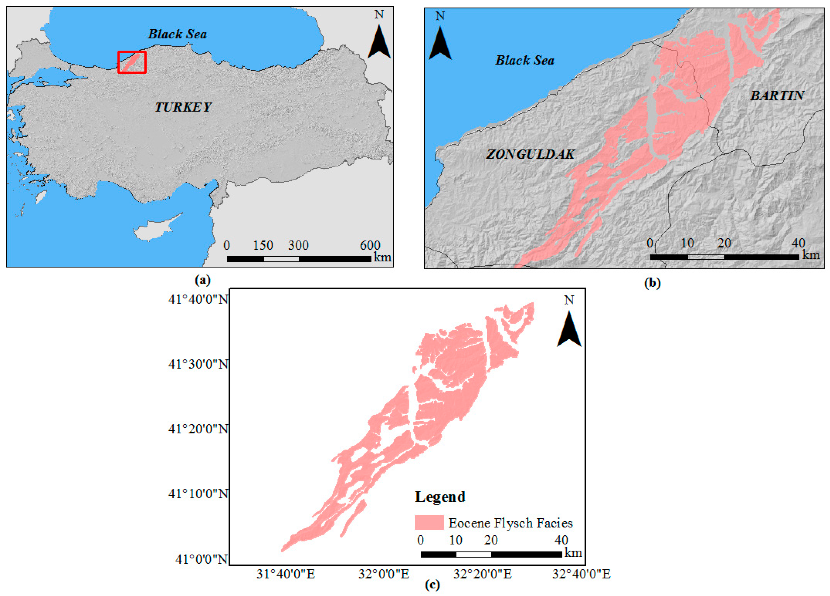
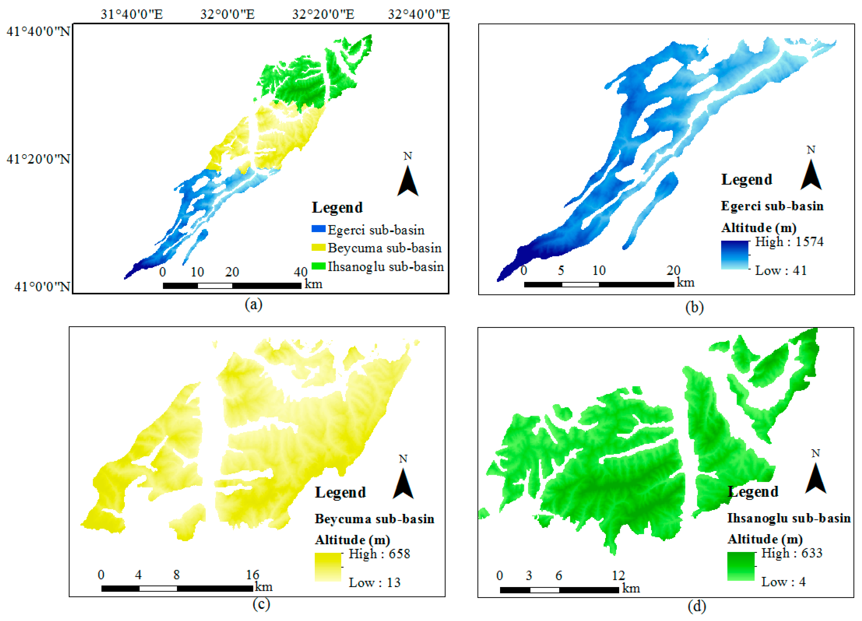
2.1. Study Area
2.2. Data Source and Pre-Processing
3. Methods
3.1. Preparation of Shallow Landslide Susceptibility Map
3.2. Determination of Shallow Landslide Initiations
3.3. Shallow Landslide Runout Distance Assessment Methodology
3.4. Selection of Model Parameters
4. Results
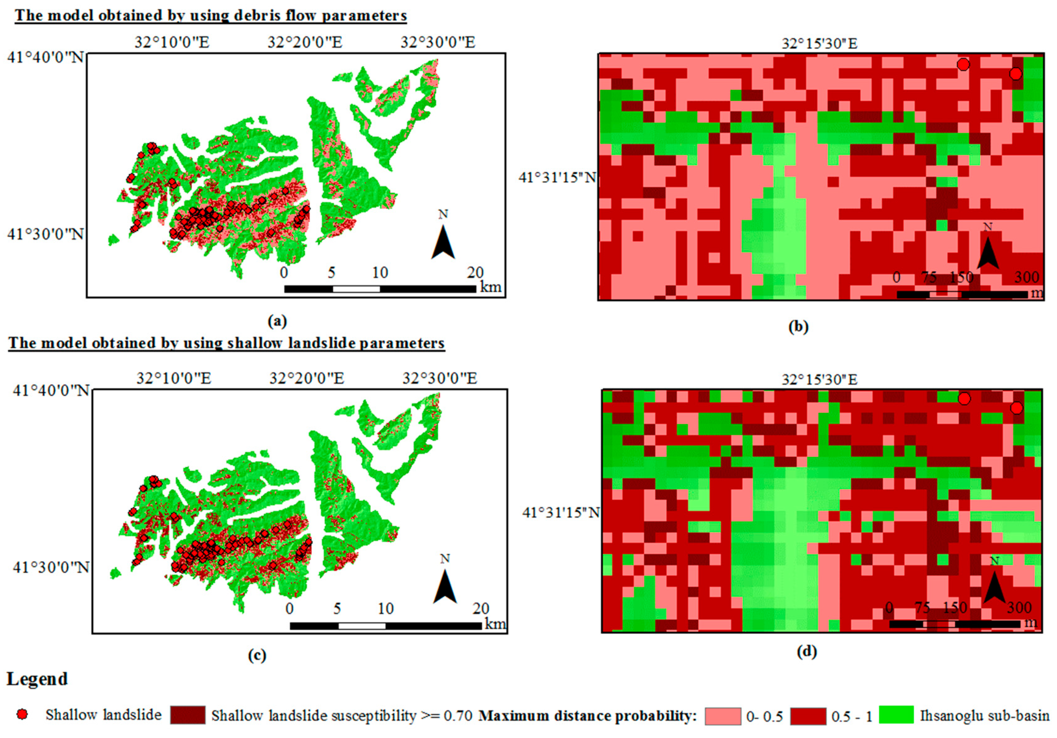
4.1. Shallow Landslide Runout Distance Assessment
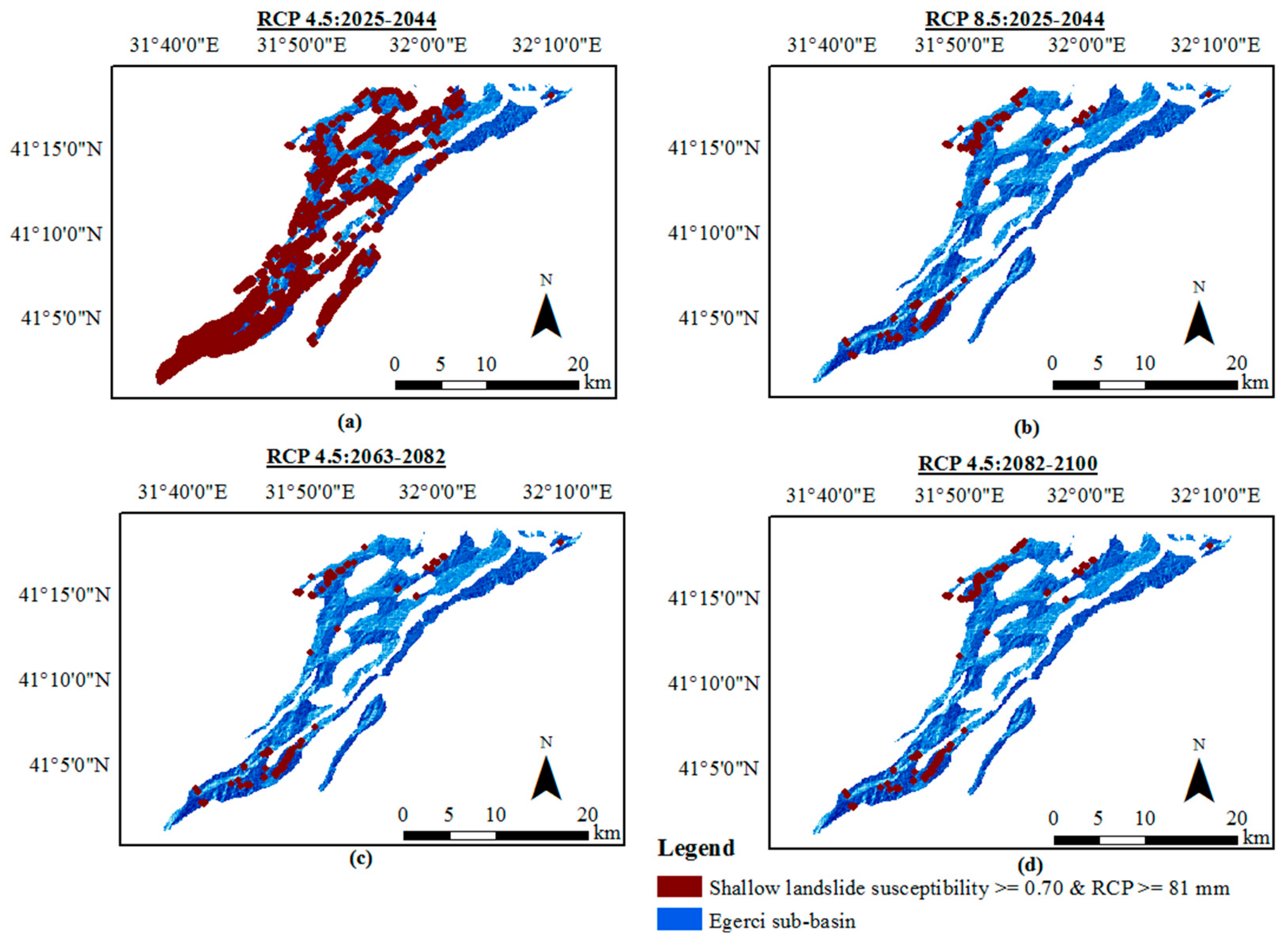
4.2. Shallow Landslide Runout Distance Assessment Considering RCP Scenarios
5. Discussion
Limitations of this Study
6. Conclusions
Author Contributions
Funding
Data Availability Statement
Acknowledgments
Conflicts of Interest
References
- Kritikos, T.; Davies, T. Assessment of Rainfall-Generated Shallow Landslide/Debris-Flow Susceptibility and Runout Using a GIS-Based Approach: Application to Western Southern Alps of New Zealand. Landslides 2015, 12, 1051–1075. [Google Scholar] [CrossRef]
- Giano, S.I.; Pescatore, E.; Siervo, V. Morphometry and Debris-Flow Susceptibility Map in Mountain Drainage Basins of the Vallo Di Diano, Southern Italy. Remote Sens. 2021, 13, 3254. [Google Scholar] [CrossRef]
- Poltnig, W.; Bak, R.; Berg, W.; Keršmanc, T. Runout-Modelling of Shallow Landslides in Carinthia (Austria). Aust. J. Earth Sci. 2016, 109, 59–67. [Google Scholar] [CrossRef]
- Kaafarani, R.; Jaoude, G.A.; Wartman, J.; Tawk, M. Landslide Susceptibility Mapping Based on Triggering Factors Using a Multi-Modal Approach. In MATEC Web Conference, Proceedings of the International Conference of Engineering Risk, Beirut, Lebanon, 3–5 April 2019; Chehade, F.H., Ed.; EDP Sciences: Les Ulis Cedex, France, 2019; Volume 281, pp. 1–8. [Google Scholar] [CrossRef]
- Mergili, M.; Schwarz, L.; Kociu, A. Combining Release and Runout in Statistical Landslide Susceptibility Modeling. Landslides 2019, 16, 2151–2165. [Google Scholar] [CrossRef]
- Zhou, W.; Fang, J.; Tang, C.; Yang, G. Empirical Relationships for The Estimation of Debris Flow Runout Distances on Depositional Fans in The Wenchuan Earthquake Zone. J. Hydrol. 2019, 577, 123932. [Google Scholar] [CrossRef]
- Apriani, D.W.; Credidi, C.; Khala, S. An Empirical-Statistical Model for Landslide Runout Distance Prediction in Indonesia. Tahun 2022, 27, 1. [Google Scholar] [CrossRef]
- Di Napoli, M.; Martire, D.D.; Bausilio, G.; Calcaterra, D.; Confuorto, P.; Firpo, M.; Pepe, G.; Cevasco, A. Rainfall-Induced Shallow Landslide Detachment, Transit and Runout Susceptibility Mapping by Integrating Machine Learning Techniques and GIS-based Approaches. Water 2021, 13, 488. [Google Scholar] [CrossRef]
- Guthrie, R.; Befus, A. DebrisFlow Predictor: An Agent-Based Runout Program for Shallow Landslides. Nat. Hazards Earth Syst. Sci. 2021, 21, 1029–1049. [Google Scholar] [CrossRef]
- Ju, L.-Y.; Xiao, T.; He, J.; Wang, H.-J.; Zhang, L.-M. Predicting Landslide Runout Paths Using Terrain Matching-Targeted Machine Learning, Engineering. Geology 2022, 311, 106902. [Google Scholar] [CrossRef]
- Giarola, A.; Meisina, C.; Tarolli, P.; Zucca, F.; Galve, J.P.; Bordoni, M. A Data-Driven Method for the Estimation of Shallow Landslide Runout. CATENA 2024, 234, 107573. [Google Scholar] [CrossRef]
- Baselt, I.; Queiroz de Oliveira, G.; Fischer, J.-T.; Pudasaini, S.P. Evolution of Stony Debris Flows in Laboratory Experiments. Geomorphology 2021, 372, 107431. [Google Scholar] [CrossRef]
- Gao, Y.; Li, B.; Zhang, H.; Wu, W.; Li, J.; Yin, Y. Numerical Modeling of Mixed Two-Phase in Long Runout Flow-Like Landslide Using LPF3D. Landslides 2023, 21, 641–660. [Google Scholar] [CrossRef]
- Yang, L.; Wei, Y.; Wang, W.; Zhu, S. Numerical Runout Modeling Analysis of the Loess Landslide at Yining, Xinjiang, China. Water 2019, 11, 1324. [Google Scholar] [CrossRef]
- Chae, B.-G.; Wu, Y.-H.; Liu, K.-F.; Choi, J.; Park, H.-J. Simulation of Debris-Flow Runout Near a Construction Site in Korea. Appl. Sci. 2020, 10, 6079. [Google Scholar] [CrossRef]
- Calista, M.; Menna, V.; Mancinelli, V.; Sciarra, N.; Miccadei, E. Rockfall and Debris Flow Hazard Assessment in the SW Escarpment of Montagna del Morrone Ridge (Abruzzo, Central Italy). Water 2020, 12, 1206. [Google Scholar] [CrossRef]
- Abraham, M.T.; Satyam, N.; Reddy, S.K.P.; Pradhan, B. Runout Modeling and Calibration of Friction Parameters of Kurichermala Debris Flow, India. Landslides 2021, 18, 737–754. [Google Scholar] [CrossRef]
- Dash, R.K.; Kanungo, D.P.; Malet, J.P. Runout Modelling and Hazard Assessment of Tangni Debris Flow in Garhwal Himalayas, India. Environ. Earth Sci. 2021, 80, 338. [Google Scholar] [CrossRef]
- Vicari, H.; Nordal, S.; Thakur, V. The Significance of Entrainment on Debris Flow Modelling: The Case of Hunnedalen, Norway. In Challenges and Innovations in Geomechanics, IACMAG 2021; Barla, M., Di Donna, A., Sterpi, D., Eds.; Lecture Notes in Civil Engineering; Springer: Cham, Switzerland, 2021; Volume 126, ISBN 978-3-030-64517-5. [Google Scholar] [CrossRef]
- Mikoš, M.; Bezak, N. Debris Flow Modelling Using RAMMS Model in the Alpine Environment with Focus on the Model Parameters and Main Characteristics. Front. Earth Sci. 2021, 8, 605061. [Google Scholar] [CrossRef]
- Oh, C.-H.; Choo, K.-S.; Go, C.-M.; Choi, J.-R.; Kim, B.-S. Forecasting of Debris Flow Using Machine Learning-Based Adjusted Rainfall Information and RAMMS Model. Water 2021, 13, 2360. [Google Scholar] [CrossRef]
- Zhou, W.; Qiu, H.; Wang, L.; Pei, Y.; Tang, B.; Ma, S.; Yang, D.; Cao, M. Combining Rainfall-Induced Shallow Landslides and Subsequent Debris Flows for Hazard Chain Prediction. CATENA 2022, 213, 106199. [Google Scholar] [CrossRef]
- Alene, G.H.; Vicari, H.; Irshad, S.; Perkis, A.; Bruland, O.; Thakur, V. Realistic Visualization Of Debris Flow Type Landslides Through Virtual Reality. Landslides 2023, 20, 13–23. [Google Scholar] [CrossRef]
- La Porta, G.; Leonardi, A.; Pirulli, M.; Cafaro, F.; Castelli, F. Time-Resolved Triggering and Runout Analysis of Rainfall-Induced Shallow Landslides. Acta Geotech. 2023. [Google Scholar] [CrossRef]
- Zhu, C.; He, M.; Karakus, M.; Zhang, X.; Tao, Z. Numerical Simulations of the Failure Process of Anaclinal Slope Physical Model and Control Mechanism of Negative Poisson’s Ratio Cable. Bull. Eng. Geol. Environ. 2021, 80, 3365–3380. [Google Scholar] [CrossRef]
- Clark, B. Numerical Modelling of Debris Flow Hazards using Computational Fluid Dynamics. Master’s Thesis, Norwegian University of Science and Technology, Trondheim, Norway, 2018. [Google Scholar]
- Melo, R.; van Asch, T.; Zêzere, J.L. Debris Flow Run-Out Simulation and Analysis Using a Dynamic Model. Nat. Hazards Earth Syst. Sci. 2018, 18, 555–570. [Google Scholar] [CrossRef]
- Gan, J.J.; Zhang, Y.X. Numerical Simulation of Debris Flow Runout Using Ramms: A Case Study of Luzhuang Gully in China. CMES 2019, 121, 981–1009. [Google Scholar] [CrossRef]
- Peruzzetto, M.; Mangeney, A.; Grandjean, G.; Levy, C.; Thiery, Y.; Rohmer, J.; Lucas, A. Operational Estimation of Landslide Runout: Comparison of Empirical and Numerical Methods. Geosciences 2020, 10, 424. [Google Scholar] [CrossRef]
- Zhu, C.; He, M.; Karakus, M.; Cui, X.; Tao, Z. Investigating Toppling Failure Mechanism of Anti-Dip Layered Slope due to Excavation by Physical Modelling. Rock. Mech. Rock. Eng. 2020, 53, 5029–5050. [Google Scholar] [CrossRef]
- Wei, L.; Cheng, H.; Dai, Z. Propagation Modeling of Rainfall-Induced Landslides: A Case Study of the Shaziba Landslide in Enshi, China. Water 2023, 15, 424. [Google Scholar] [CrossRef]
- Iverson, R.M. Scaling and Design of Landslide and Debris-Flow Experiments. Geomorphology 2015, 244, 9–20. [Google Scholar] [CrossRef]
- Khalkhali, A.B.; Koochaksaraei, M.K. Evaluation of Limit Equilibrium and Finite Element Methods in Slope Stability Analysis Case Study of Zaremroud Landslide, Iran. Comput. Eng. Phys. Model. 2019, 2, 1–15. [Google Scholar]
- Guo, J.; Cui, Y.; Xu, W.; Yin, Y.; Li, Y.; Jin, W. Numerical Investigation of the Landslide-Debris Flow Transformation Process Considering Topographic and Entrainment Effects: A Case Study. Landslides 2022, 19, 773–788. [Google Scholar] [CrossRef]
- Milledge, D.G.; Densmore, A.L.; Bellugi, D.; Rosser, N.J.; Watt, J.; Li, G.; Oven, K.J. Simple Rules to Minimise Exposure to Coseismic Landslide Hazard. Nat. Hazards Earth Syst. Sci. 2019, 19, 837–856. [Google Scholar] [CrossRef]
- Vadivel, S.; Sennimalai, C.S. Failure Mechanism of Long-Runout Landslide Triggered by Heavy Rainfall in Achanakkal, Nilgiris, India. J. Geotech. Geoenviron. Eng. 2019, 145, 04019047. [Google Scholar] [CrossRef]
- Ali, S.; Haider, R.; Abbas, W. Empirical Assessment of Rockfall and Debris Flow Risk along the Karakoram Highway, Pakistan. Nat. Hazards 2021, 106, 2437–2460. [Google Scholar] [CrossRef]
- Sturzenegger, M.; Holm, K.; Lau, C.; Jakob, M. Semi-Automated Regional Scale Debris-Flow and Debris-Flood Susceptibility Mapping Based on Digital Elevation Model Metrics and Flow-R Software. In Proceedings of the 7th International Conference on Debris-Flow Hazards Mitigation, Golden, CO, USA, 10–13 June 2019. [Google Scholar]
- Pradhan, A.M.S. Quantification of Slope Unit Wise Vulnerability in Terms of Building Aggregation. WRRDC Res. Lett. 2021, 7, 1–2. [Google Scholar]
- Quinn, P.; Beven, K.; Chevallier, P.; Planchon, O. The Prediction of Hillslope Flow Paths for Distributed Hydrological Modelling Using Digital Terrain Models. Hydrol. Process 1991, 5, 59–79. [Google Scholar] [CrossRef]
- Holmgren, P. Multiple Flow Direction Algorithms for Runoff Modelling in Grid Based Elevation Models: An Empirical Evaluation. Hydrol. Process 1994, 8, 327–334. [Google Scholar] [CrossRef]
- Horton, P.; Jaboyedoff, M.; Rudaz, B.; Zimmermann, M. Flow-R, a Model for Susceptibility Mapping of Debris Flows and other Gravitational Hazards at a Regional Scale. Nat. Hazards 2013, 13, 869–885. [Google Scholar] [CrossRef]
- Guthrie, R.H.; Deadman, P.; Cabrera, R.; Evans, S.G. Exploring the Magnitude-Frequency Distribution: A Cellular Automata Model for Landslides. Landslides 2008, 5, 151–159. [Google Scholar] [CrossRef]
- Gamma, P. dfwalk—Ein Murgang-Simulationsprogramm zur Gefahrenzonierung. In Geographica Bernensia G66; University of Bern: Bern, German, 2000. [Google Scholar]
- Mergili, M.; Krenn, J.; Chu, H.-J. r.randomwalk v1, A Multi-Functional Conceptual Tool for Mass Movement Routing. Geosci. Model. Dev. 2015, 8, 4027–4043. [Google Scholar] [CrossRef]
- Pastorello, R.; Michelini, T.; D’Agostino, V. On the Criteria to Create a Susceptibility Map to Debris Flow at a Regional Scale Using Flow-R. J. Mt. Sci. 2017, 14, 621–635. [Google Scholar] [CrossRef]
- McCoy, K.M. Debris-Flow Susceptibility Mapping in Colorado using Flow-R: Calibration Techniques and Selected Examples. In Proceedings of the 7th International Conference on Debris-Flow Hazards Mitigation, Golden, CO, USA, 10–13 June 2019. [Google Scholar]
- Paudel, B.P. GIS-Based Assessment of Debris Flow Susceptibility and Hazard in Mountainous Regions of Nepal. Ph.D. Thesis, Ottawa University, Ottawa, ON, Canada, 2019. [Google Scholar]
- Do, H.M.; Yin, K.L.; Guo, Z.Z. A comparative study on the integrative ability of the analytical hierarchy process, weights of evidence and logistic regression methods with the Flow-R model for landslide susceptibility assessment. Geomat. Nat. Haz. Risk 2020, 11, 2449–2485. [Google Scholar] [CrossRef]
- Charbel, L.; El Hage Hassan, H. Mudflow Modeling Using Flow-R Software: Case Study of Ras Baalbek Basin (Lebanon). Geo-Eco-Trop 2021, 45, 475–486. [Google Scholar]
- Jiang, N.; Su, F.; Li, Y.; Guo, X.; Zhang, J.; Liu, X. Debris Flow Assessment in the Gaizi-Bulunkou Section of Karakoram Highway. Front. Earth Sci. 2021, 9, 660579. [Google Scholar] [CrossRef]
- Liu, J.; Wu, Y.; Gao, X.; Zhang, X. A Simple Method of Mapping Landslides Runout Zones Considering Kinematic Uncertainties. Remote Sens. 2022, 14, 668. [Google Scholar] [CrossRef]
- Putra, M.; Dinata, I.; Sadisun, I.; Sarah, D.; Aulia, A.; Sukristiyanti, S. Modeling of Individual Debris Flows Based on DEMNAS Using Flow-R: A Case Study in Sigi. Central Sulawesi. RISET Geol. Dan Pertamb. 2022, 32, 37–58. [Google Scholar] [CrossRef]
- Xu, H.; Su, P.; Chen, Q.; Liu, F.; Zhou, Q.; Liu, L. Susceptibility Areas Identification and Risk Assessment of Debris Flow Using the Flow-R Model: A Case Study of Basu County of Tibet. Geoenviron. Disasters 2022, 9, 13. [Google Scholar] [CrossRef]
- Berti, M.; Simoni, A. DFLOWZ: A Free Program to Evaluate the Area Potentially Inundated by a Debris Flow. Comput. Geosci. 2014, 67, 14–23. [Google Scholar] [CrossRef]
- Gorr, A.N.; McGuire, L.A.; Youberg, A.M.; Rengers, F.K. A Progressive Flow-Routing Model for Rapid Assessment of Debris-Flow Inundation. Landslides 2022, 19, 2055–2073. [Google Scholar] [CrossRef]
- Wang, X.; Yin, J.; Luo, M.; Ren, H.; Li, J.; Wang, L.; Li, D.; Li, G. Active High-Locality Landslides in Mao County: Early Identification and Deformational Rules. J. Earth Sci. 2023, 34, 1596–1615. [Google Scholar] [CrossRef]
- Pradhan, A.M.S.; Kang, H.; Lee, S.; Kim, Y. Spatial Model Integration for Shallow Landslide Susceptibility and Its Runout Using a GIS-Based Approach in Yongin, Korea. Geocarto Int. 2017, 32, 420–441. [Google Scholar] [CrossRef]
- Rahman, M.S.; Ahmed, B.; Di, L.P. Landslide Initiation and Runout Susceptibility Modeling in the Context of Hill Cutting and Rapid Urbanization: A Combined Approach of Weights of Evidence and Spatial Multi-Criteria. J. Mt. Sci. 2017, 14, 1919–1937. [Google Scholar] [CrossRef]
- Polat, A.; Erik, D. Debris Flow Susceptibility and Propagation Assessment in West Koyulhisar, Turkey. J. Mt. Sci. 2020, 17, 2611–2623. [Google Scholar] [CrossRef]
- Park, D.; Lee, S.; Nikhil, N.V.; Kang, S.; Park, J. Debris Flow Hazard Zonation by Probabilistic Analysis (Mt. Woomyeon, Seoul, Korea). Int. J. Innov. Res. Sci. Eng. Technol. 2013, 2, 2381–2390. [Google Scholar]
- Bera, S.; Melo, R.; Guru, B. Assessment of Exposed Elements in a Changing Built Environment by Using an Integrated Model of Debris Flow Initiation and Runout (Kalimpong Region, Himalaya). Bull. Eng. Geol. Environ. 2021, 80, 7131–7152. [Google Scholar] [CrossRef]
- Sharma, C.P.; Kumar, A.; Chahal, P.; Shukla, U.K.; Srivastava, P.; Jaiswal, M.K. Debris Flow Susceptibility Assessment of Leh Valley, Ladakh, Based on Concepts of Connectivity, Propagation and Evidence-Based Probability. Nat. Hazards 2023, 115, 1833–1859. [Google Scholar] [CrossRef]
- Guo, J.; Wang, J.; Li, Y.; Yi, S. Discussions on the Transformation Conditions of Wangcang Landslide-Induced Debris Flow. Landslides 2021, 18, 1833–1843. [Google Scholar] [CrossRef]
- Ageenko, A.; Hansen, L.C.; Lyng, K.L.; Bodum, L.; Arsanjani, J.J. Landslide Susceptibility Mapping Using Machine Learning: A Danish Case Study. ISPRS Int. J. Geo-Inf. 2022, 11, 324. [Google Scholar] [CrossRef]
- Araújo, J.R.; Ramos, A.M.; Soares, P.M.M.; Melo, R.; Oliveira, S.C.; Trigo, R.M. Impact of Extreme Rainfall Events on Landslide Activity in Portugal Under Climate Change Scenarios. Landslides 2022, 19, 2279–2293. [Google Scholar] [CrossRef]
- Nefros, C.; Tsagkas, D.S.; Kitsara, G.; Loupasakis, C.; Giannakopoulos, C. Landslide Susceptibility Mapping under the Climate Change Impact in the Chania Regional Unit, West Crete, Greece. Land 2023, 12, 154. [Google Scholar] [CrossRef]
- Chen, Y.; Chen, E.; Zhang, J.; Zhu, J.; Xiao, Y.; Dai, Q. Investigation of Model Uncertainty in Rainfall-Induced Landslide Prediction under Changing Climate Conditions. Land 2023, 12, 1732. [Google Scholar] [CrossRef]
- Guo, Z.; Ferrer, J.V.; Hürlimann, M.; Medina, V.; Puig-Polo, C.; Yin, K.; Huang, D. Shallow Landslide Susceptibility Assessment Under Future Climate and Land Cover Changes: A case Study from Southwest China. Geosci. Front. 2023, 14, 101542. [Google Scholar] [CrossRef]
- Akbas, B.; Akdeniz, N.; Aksay, A.; Altun, İ.E.; Balcı, V.; Bilginer, E.; Bilgiç, T.; Duru, M.; Ercan, T.; Gedik, İ.; et al. 1:1250,000 olcekli Türkiye jeoloji haritasi. Maden Tetk. Ve Aram. Genel Mudurlugu Yayin. 2011, 12p. [Google Scholar]
- Turkish State Meteorological Service. Maximum Rainfall Intensity and Recurrence Analysis. Available online: https://mgm.gov.tr/veridegerlendirme/maksimum-yagislar.aspx (accessed on 23 December 2022).
- Can, T.; Nefeslioglu, H.A.; Gokceoglu, C.; Sonmez, H.; Duman, T.Y. Susceptibility Assessments of Shallow Earthflows Triggered by Heavy Rainfall at Three Catchments by Logistic Regression Analyses. Geomorphology 2005, 72, 250–271. [Google Scholar] [CrossRef]
- Turkish State Meteorological Service. Daily Historical Precipitation (mm=kg/m2) OMGİ and MANUEL, 2023, Data Sheets provided by Turkish State Meteorological Service.
- Akgun, A.; Gorum, T.; Nefeslioglu, H. Landslide Size Distribution Characteristics of Cretaceous and Eocene Flysch Assemblages in the Western Black Sea Region of Turkey. In Understanding and Reducing Landslide Disaster Risk; Guzzetti, F., Arbanas, S.M., Eds.; Springer: London, UK; Berlin/Heidelberg, Germany, 2021; Volume 2, pp. 299–303. [Google Scholar] [CrossRef]
- Turkish State Meteorological Service. Daily Total Precipitation (mm). Available online: https://www.mgm.gov.tr/sondurum/toplam-yagis.aspx (accessed on 21 November 2023).
- Varnes, D.J. Slope movement types and processes. In Special Report 176: Landslides: Analysis and Control; Schuster, R.L., Krizek, R.J., Eds.; Transportation and Road Research Board, National Academy of Science: Washington, DC, USA, 1978; pp. 11–33. [Google Scholar]
- CORINE Land Cover Change 2012–2018 (Vector/Raster 100 m), Europe, 6-Yearly, CLC 2018 Version v2020 20u1. Available online: https://land.copernicus.eu/pan-european/corine-land-cover/lcc-2012-2018?tab=download (accessed on 16 August 2022).
- Duman, T.; Emre, O.; Can, T.; Nefeslioglu, H.A.; Kecer, M.; Dogan, A.; Durmaz, S.; Ates, S. Türkiye Heyelan Envanteri Haritasi, 1/500,000 olcekli Zonguldak Paftasi. Maden Tetkik ve Arama Genel Mudurlugu (MTA). Ozel Yayinlar Serisi 2005, 4a, 10p. [Google Scholar]
- Duman, T.Y.; Can, T.; Emre, O.; Kecer, M.; Dogan, A.; Ates, S.; Durmaz, S. Landslide Inventory of Northwestern Anatolia, Turkey. J. Eng. Geol. 2005, 77, 99–114. [Google Scholar] [CrossRef]
- Duman, T.Y.; Can, T.; Emre, O. 1/1500000 olcekli Türkiye Heyelan Envanteri Haritasi. Maden Tetkik ve Arama Genel Mudurlugu (MTA) Ozel Yayinlar Serisi 2011, 27, 12p. [Google Scholar]
- Hovius, N.; Stark, C.P.; Allen, P.A. Sediment Flux from a Mountain Belt Derived by Landslide Mapping. Geology 1997, 25, 231–234. [Google Scholar] [CrossRef]
- Jaboyedoff, M.; Carrea, D.; Derron, M.H.; Thierry, O.; Penna, I.; Bejamin, R. A Review of Methods Used to Estimate Initial Landslide Failure Surface Depths and Volumes. Eng. Geol. 2020, 267, 105478. [Google Scholar] [CrossRef]
- Zaruba, Q.; Mencl, V. Landslides and Their Control; Elsevier: Amsterdam, The Netherlands, 1969. [Google Scholar]
- Nefeslioglu, H.A.; Gokceoglu, C. Probabilistic Risk Assessment in Medium Scale for Rainfall Induced Earthflows: Catakli Catchment Area (Cayeli, Rize, Turkey). Math Probl. Eng. 2011, 2011, 280431. [Google Scholar] [CrossRef]
- Kalantar, B.; Pradhan, B.; Naghibi, S.A.; Motevalli, A.; Mansor, S. Assessment of the Effects of Training Data Selection on the Landslide Susceptibility Mapping: A Comparison between Support Vector Machine (SVM), Logistic Regression (LR) and Artificial Neural Networks (ANN). Geomat. Nat. Haz. Risk 2018, 9, 49–69. [Google Scholar] [CrossRef]
- Nhu, V.-H.; Shirzadi, A.; Shahabi, H.; Singh, S.K.; Al-Ansari, N.; Clague, J.J.; Jaafari, A.; Chen, W.; Miraki, S.; Dou, J.; et al. Shallow Landslide Susceptibility Mapping: A Comparison between Logistic Model Tree, Logistic Regression, Naïve Bayes Tree, Artificial Neural Network, and Support Vector Machine Algorithms. Int. J. Environ. Res. Public Health 2020, 17, 2749. [Google Scholar] [CrossRef]
- Crawford, M.M.; Dortch, J.M.; Koch, H.J.; Killen, A.A.; Zhu, J.; Zhu, Y.; Bryson, L.S.; Haneberg, W.C. Using Landslide-Inventory Mapping for a Combined Bagged-Trees and Logistic-Regression Approach to Determining Landslide Susceptibility in Eastern Kentucky, USA. Q. J. Eng. Geol. Hydrogeol. 2021, 54, qjegh2020-177. [Google Scholar] [CrossRef]
- Crawford, M.M.; Dortch, J.M.; Koch, H.J.; Zhu, Y.; Haneberg, W.C.; Wang, Z.; Bryson, L.S. Landslide Risk Assessment in Eastern Kentucky. USA: Developing a Regional Scale, Limited Resource Approach. Remote Sens. 2022, 14, 6246. [Google Scholar] [CrossRef]
- Dashbold, B.; Bryson, L.S.; Crawford, M.M. Landslide Hazard and Susceptibility Maps Derived from Satellite and Remote Sensing Data Using Limit Equilibrium Analysis and Machine Learning Model. Nat. Hazards 2022, 116, 235–265. [Google Scholar] [CrossRef]
- Nwazelibe, V.; Unigwe, C.; Egbueri, J. Integration and Comparison of Algorithmic Weight of Evidence and Logistic Regression in Landslide Susceptibility Mapping of the Orumba North Erosion-Prone Region, Nigeria. Model Earth Syst. Environ. 2022, 9, 967–986. [Google Scholar] [CrossRef]
- Polykretis, C.; Chalkias, C. Comparison and Evaluation of Landslide Susceptibility Maps Obtained from Weight of Evidence, Logistic Regression, and Artificial Neural Network Models. Nat. Hazards 2018, 93, 249–274. [Google Scholar] [CrossRef]
- Menard, S. Applied Logistic Regression Analysis; Sage University Paper Series on Quantitative Applications in Social Sciences, Sage Publications No. 106; SAGE Publications: Thousand Oaks, CA, USA, 1995. [Google Scholar]
- Ghasemian, B.; Shahabi, H.; Shirzadi, A.; Al-Ansari, N.; Jaafari, A.; Geertsema, M.; Melesse, A.M.; Singh, S.K.; Ahmad, A. Application of a Novel Hybrid Machine Learning Algorithm in Shallow Landslide Susceptibility Mapping in a Mountainous Area. Front. Environ. Sci. 2022, 10, 897254. [Google Scholar] [CrossRef]
- Xie, W.; Li, X.; Jian, W.; Yang, Y.; Liu, H.; Robledo, L.F.; Nie, W. A Novel Hybrid Method for Landslide Susceptibility Mapping-Based GeoDetector and Machine Learning Cluster: A Case of Xiaojin County, China. ISPRS Int. J. Geo-Inf. 2021, 10, 93. [Google Scholar] [CrossRef]
- Xie, W.; Nie, W.; Saffari, P.; Robledo, L.F.; Descote, P.-Y.; Jian, W. Landslide Hazard Assessment Based on Bayesian Optimization-Support Vector Machine in Nanping City, China. Nat. Hazards 2021, 109, 931–948. [Google Scholar] [CrossRef]
- Karakaş, G.; Can, R.; Kocaman, S.; Nefeslioglu, H.A.; Gokceoglu, C. Landslide Susceptibility Mapping with Random Forest Model for Ordu, Turkey. Int. Arch. Photogramm. Remote Sens. Spatial Inf. Sci. 2020, XLIII-B3-2020, 1229–1236. [Google Scholar] [CrossRef]
- Ling, S.; Zhao, S.; Huang, J.; Zhang, X. Landslide Susceptibility Assessment Using Statistical and Machine Learning Techniques: A Case Study in The Upper Reaches of the Minjiang River, Southwestern China. Front. Earth Sci. 2022, 10, 986172. [Google Scholar] [CrossRef]
- NCAR Geographic Information System Program. Climate Change Scenarios. Available online: https://gis.ucar.edu/inspector (accessed on 16 August 2022).
- Sun, L.; Wei, Y.; Cai, H.; Yan, J.; Xiao, J. Improved Fast Adaptive IDW Interpolation Algorithm based on the Borehole Data Sample Characteristic and Its Application. J. Phys. Conf. Ser. 2019, 1284, 012074. [Google Scholar] [CrossRef]
- Maleika, W. Inverse distance weighting method optimization in the process of digital terrain model creation based on data collected from a multibeam echosounder. Appl. Geomat. 2020, 12, 397–407. [Google Scholar] [CrossRef]
- Mohamed Yusof, M.K.T.; A Rashid, A.S.; Abdul Khanan, M.F.; Abdul Rahman, M.Z.; Abdul Manan, W.A.; Kalatehjari, R.; Dehghanbanadaki, A. Assessing the Impact of RCP4.5 and RCP8.5 Scenarios on Landslide Susceptibility Mapping Using Support Vector Machine: A case study of Penang Island, Malaysia. Phys. Chem. Earth Parts A/B/C 2024, 133, 103496. [Google Scholar] [CrossRef]
- Nasidi, N.M.; Wayayok, A.; Abdullah, A.F.; Kassim, M.S.M. Dynamics of Potential Precipitation under Climate Change Scenarios at Cameron Highlands, Malaysia. SN Appl. Sci. 2021, 3, 334. [Google Scholar] [CrossRef]
- New Decade Brings Reference Period Change for Climate Data. Available online: https://climate.copernicus.eu/new-decade-brings-reference-period-change-climate-data (accessed on 9 October 2022).
- Park, S.J.; Lee, D. Predicting Susceptibility to Landslides Under Climate Change Impacts in Metropolitan Areas of South Korea Using Machine Learning. Geomat. Nat. Hazards Risk 2021, 12, 2462–2476. [Google Scholar] [CrossRef]
- Horton, P.; Oppikofer, T.; Michoud, C. Introduction to Flow R Online Tutorial © Terranum Ltd. Available online: https://www.terranum.ch/en/products/flow-r/ (accessed on 10 August 2022).
- Prochaska, A.B.; Santi, P.M.; Higgins, J.D.; Cannon, S.H. A Study of Methods to Estimate Debris Flow Velocity. Landslides 2008, 5, 431–444. [Google Scholar] [CrossRef]
- Nie, Y.; Li, X.; Xu, R. Dynamic Hazard Assessment of Debris Flow Based on TRIGRS and Flow-R Coupled Models. Stoch. Environ. Res. Risk Assess 2022, 36, 97–114. [Google Scholar] [CrossRef]
- Nie, Z.; Lang, Q.; Zhang, Y.; Zhang, J.; Chen, Y.; Pan, Z. Risk Assessment of Landslide Collapse Disasters along National Highways Based on Information Quantity and Random Forest Coupling Methods: A Case Study of the G331 National Highway. ISPRS Int. J. Geo-Inf. 2023, 12, 493. [Google Scholar] [CrossRef]
- Takaoka, S. A Landscape Level Study on Vegetation Richness of Ancient Landslide Areas. Prog. Phys. Geogr. 2023, 48, 1–15. [Google Scholar] [CrossRef]
- Nishioka, M.; Inoue, H.; Ota, T.; Mizoue, N. Impact of Forest Type and Age on Shallow Landslide Susceptibility a Case Study from the 2017 Heavy Rainfall in Northern Kyushu. Jpn. Socioecon. Plan. Manag. 2023, 28, 389–396. [Google Scholar] [CrossRef]
- Malla, R.; Neupane, P.R.; Köhl, M. Climate Change Impacts Vegetation Shift of Broad Leaved and Coniferous Forests. Trees For. People 2023, 14, 100457. [Google Scholar] [CrossRef]
- Yu, J.; Berry, P.; Guillod, B.P.; Hickler, T. Climate Change Impacts on the Future of Forests in Great Britain. Front. Environ. Sci. 2021, 9, 640530. [Google Scholar] [CrossRef]
- Du, Y.; Xie, M.; Jia, J. Stepped Settlement: A Possible Mechanism for Translational Landslides. Catena 2020, 187, 104365. [Google Scholar] [CrossRef]
- Grabar, K.; Jug, J.; Bek, A.; Strelec, S. Comparison of the Piezocone Penetrometer (CPTU) and Flat Dilatometer (DMT) Methods for Landslide Characterisation. Geosciences 2024, 14, 64. [Google Scholar] [CrossRef]


| Authors | Research | Landslide Initiations | Runout Method | Flow Direction Algorithm |
|---|---|---|---|---|
| Horton et al. [42], Jiang et al. [51], Xu et al. [54], Park et al. [61], Sharma et al. [63] | Debris flow runout susceptibility map | Initiations detected by Flow-R | SFLM | Modified Holmgren |
| Pastorello et al. [46], McCoy [47], Paudel [48], Putra et al. [53] | Debris flow runout susceptibility map | User-defined initiations considering flow accumulation and slope [46], landslide susceptibility map [48], and Sentinel images [53] | SFLM | Modified Holmgren |
| Ali et al. [37], Bera et al. [62] | Debris flow runout susceptibility map | User-defined initiations based on remote sensing, slope angle distribution [37], and GPS and multi-temporal satellite images [61] | SFLM | Holmgren |
| Giano et al. [2] | Debris flow runout susceptibility map | Initiations detected by Flow-R | Perla | Modified Holmgren |
| Polat and Erik [60] | Debris flow runout susceptibility map | User-defined initiations considering landslide susceptibility map | Perla | Modified Holmgren |
| Charbel and El Hage Hassan [50] | Mudflow runout susceptibility map | Initiations detected by Flow-R | SFLM | Holmgren |
| Do et al. [49] | Landslide runout susceptibility map | Initiations detected by Flow-R | SFLM | Modified Holmgren |
| Liu et al. [52] | Landslide runout susceptibility map | User-defined initiations based on previous studies and D-InSAR technology | SFLM | Modified Holmgren |
| Sub-Basin | N | Statistics | Area (m2) | Failure Depth (m) | Travel Angle (°) | Observed Runout Distance (m) |
|---|---|---|---|---|---|---|
| Egerci | 111 | Min. | 21 | 0.2 | 1 | 7 |
| Max. | 4116 | 3.2 | 49 | 122 | ||
| Mean | 536 | 1.0 | 23 | 53 | ||
| Median | 344 | 0.9 | 24 | 47 | ||
| Std. Deviation | 572 | 0.5 | 12 | 29 | ||
| Beycuma | 15 | Min. | 23 | 0.2 | 4 | 7 |
| Max. | 1843 | 2.1 | 28 | 83 | ||
| Mean | 376 | 0.9 | 13 | 36 | ||
| Median | 258 | 0.8 | 13 | 31 | ||
| Std. Deviation | 438 | 0.5 | 8 | 20 | ||
| Ihsanoglu | 136 | Min. | 7 | 0.1 | 1 | 5 |
| Max. | 1710 | 2.1 | 32 | 122 | ||
| Mean | 140 | 0.5 | 11 | 25 | ||
| Median | 65 | 0.4 | 10 | 17 | ||
| Std. Deviation | 226 | 0.3 | 7 | 21 |
| Sub-Basin | Statistics | A | SG (°) | SA (°) | PLC | PRC | CI | CD | TWI | SLF | CNBL (m) | CND (m) | VD (m) |
|---|---|---|---|---|---|---|---|---|---|---|---|---|---|
| Egerci | Min. | 41 | 0 | 0 | −0.01 | −0.01 | −92 | 0 | 2 | 0 | 41 | −49 | −3 |
| Max. | 1574 | 60 | 6.28 | 0.01 | 0.012 | 96 | 20 | 21 | 38 | 1382 | 449 | 549 | |
| Mean | 444 | 15 | 3.25 | 0 | 0 | 0 | 0 | 7 | 5 | 381 | 64 | 236 | |
| Median | 425 | 14 | 3.04 | 0 | 0 | 0 | 0 | 6 | 4 | 369 | 49 | 229 | |
| Std. Deviation | 259 | 8 | 1.91 | 0.002 | 0.002 | 8 | 1 | 2 | 3 | 233 | 60 | 133 | |
| Beycuma | Min. | 13 | 0 | 0 | −0.01 | −0.01 | −100 | 0 | 3 | 0 | 13 | −27 | 0 |
| Max. | 658 | 52 | 6.28 | 0.008 | 0.009 | 100 | 19 | 20 | 24 | 444 | 304 | 277 | |
| Mean | 170 | 11 | 3.27 | 0 | 0 | 0 | 0 | 7 | 3 | 129 | 41 | 140 | |
| Median | 158 | 9 | 3.33 | 0 | 0 | 0 | 0 | 7 | 2 | 118 | 32 | 146 | |
| Std. Deviation | 91 | 6 | 1.91 | 0.001 | 0.001 | 9 | 1 | 2 | 2 | 69 | 38 | 61 | |
| Ihsanoglu | Min. | 4 | 0 | 0 | −0.01 | −0.02 | −98 | 0 | 2 | 0 | 6 | −39 | 0 |
| Max. | 633 | 70 | 6.28 | 0.017 | 0.021 | 92 | 32 | 20 | 30 | 284 | 468 | 339 | |
| Mean | 121 | 11 | 3.35 | 0 | 0 | 0 | 0 | 7 | 3 | 79 | 42 | 117 | |
| Median | 104 | 10 | 3.43 | 0 | 0 | 0 | 0 | 6 | 2 | 69 | 32 | 117 | |
| Std. Deviation | 71 | 7 | 1.83 | 0.001 | 0.001 | 10 | 1 | 2 | 2 | 43 | 42 | 51 |
| Sub-Basin | Failure | Flow Direction Algorithm | x | dh (m) | Travel Angle (°) | Velocity (m/s) |
|---|---|---|---|---|---|---|
| Egerci | Debris flow | Modified Holmgren | 4 | 1 | 24 | 15 |
| Shallow landslides | Modified Holmgren | 25 | 1 | 24 | 15 | |
| Beycuma | Debris flow | Modified Holmgren | 4 | 1 | 13 | 15 |
| Shallow landslides | Modified Holmgren | 25 | 1 | 13 | 15 | |
| Ihsanoglu | Debris flow | Modified Holmgren | 4 | 1 | 10 | 15 |
| Shallow landslides | Modified Holmgren | 25 | 1 | 10 | 15 |
Disclaimer/Publisher’s Note: The statements, opinions and data contained in all publications are solely those of the individual author(s) and contributor(s) and not of MDPI and/or the editor(s). MDPI and/or the editor(s) disclaim responsibility for any injury to people or property resulting from any ideas, methods, instructions or products referred to in the content. |
© 2024 by the authors. Licensee MDPI, Basel, Switzerland. This article is an open access article distributed under the terms and conditions of the Creative Commons Attribution (CC BY) license (https://creativecommons.org/licenses/by/4.0/).
Share and Cite
Komu, M.P.; Nefeslioglu, H.A.; Gokceoglu, C. Modeling Shallow Landslide Runout Distance in Eocene Flysch Facies Using Empirical–Statistical Models (Western Black Sea Region of Türkiye). ISPRS Int. J. Geo-Inf. 2024, 13, 84. https://doi.org/10.3390/ijgi13030084
Komu MP, Nefeslioglu HA, Gokceoglu C. Modeling Shallow Landslide Runout Distance in Eocene Flysch Facies Using Empirical–Statistical Models (Western Black Sea Region of Türkiye). ISPRS International Journal of Geo-Information. 2024; 13(3):84. https://doi.org/10.3390/ijgi13030084
Chicago/Turabian StyleKomu, Muge Pinar, Hakan Ahmet Nefeslioglu, and Candan Gokceoglu. 2024. "Modeling Shallow Landslide Runout Distance in Eocene Flysch Facies Using Empirical–Statistical Models (Western Black Sea Region of Türkiye)" ISPRS International Journal of Geo-Information 13, no. 3: 84. https://doi.org/10.3390/ijgi13030084