Article

Exploring the Spatiotemporal Effects of the Built Environment on the Nonlinear Impacts of Metro Ridership: Evidence from Xi’an, China

1
School of Architecture, Chang’an University, Xi’an 710061, China
2
Engineering Research Center of Collaborative Planning of Low-Carbon Urban Space and Transportation, Universities of Shaanxi Province, Xi’an 710061, China
3
School of Telecommunications Engineering, Xidian University, Xi’an 710071, China
*
Author to whom correspondence should be addressed.
ISPRS Int. J. Geo-Inf. 2024, 13(3), 105; https://doi.org/10.3390/ijgi13030105
Submission received: 25 December 2023 / Revised: 28 February 2024 / Accepted: 18 March 2024 / Published: 21 March 2024

Abstract

:
Exploring the correlation of the built environment with metro ridership is vital for fostering sustainable urban growth. Although the research conducted in the past has explored how ridership is nonlinearly influenced by the built environment, less research has focused on the spatiotemporal ramifications of these nonlinear effects. In this study, density, diversity, distance, destination, and design parameters are utilized to depict the “5D” traits of the built environment, while Shapley Additive Explanations with eXtreme Gradient Boosting (XGBoost-SHAP) are adopted to uncover the spatial and temporal features concerning the nonlinear relationship of the built environment with ridership for metro stations located in Xi’an. We conducted a K-means clustering analysis to detect different site clusters by utilizing local SHAP coefficients. The results show that (1) built environment variables significantly influence metro ridership in a nonlinear manner at different periods and thresholds, with the POI facility density being the most critical variable and the other variables demonstrating time-driven effects; (2) the variables of population density and parking lot density exhibit spatial impact heterogeneity, while the number of parks and squares do not present a clear pattern; and (3) based on the clustering results, the metro stations are divided into four categories, and differentiated guidance strategies and planning objectives are proposed. Moreover, the current work offers a more developed insight into the spatiotemporal influence of built environments on metro travel in Xi’an, China, using nonlinear modeling, which has vital implications for coordinated urban–metro development.

1. Introduction

At present, numerous cities worldwide are grappling with the so-called “big city diseases” that stem from the rapid urbanization process, including traffic jams and transportation difficulties, as well as environmental contamination. Consequently, urban design interventions aimed at lowering vehicle operation and associated city issues have been a focal point of academic research [1,2]. To promote green transportation in large cities, the prioritized development of public transport, like urban metros, along with advocacy for preferable urban development, have emerged as the most appropriate choices. Moreover, urban metro buildings located in China have ushered in a fast growth era. Pedestrian catchment areas (PCAs) in metro stations are popular gathering places for urban residential, occupational, and commercial establishments, whose built environmental traits, including land utilization, block design, and establishment arrangement, are influential for stations’ ridership distribution [3,4,5]. Therefore, explaining the correlation of ridership with the urban built environment helps us to improve the level of urban space–metro station coordination, helping us to achieve a sustainable developmental pattern for urban transportation.
To date, numerous studies in the field have employed the direct ridership model (DRM) [6,7,8,9,10], which presumes a linear relationship between these variables. However, the practical application and verification of this model, particularly in the context of metro stations, present significant challenges to the research. However, empirical evidence on the key variables and optimal thresholds is required to address the question of what changes in the built environment can facilitate or inhibit ridership outcomes. Exploration of the nonlinear correlation of the built environment with travel behavior is not a novel idea [11,12,13]. Recent studies have successfully demonstrated this nonlinear relationship at a global scale and identified the relevant thresholds. Nevertheless, spatial heterogeneity can introduce instability into this nonlinear relationship [14]. Moreover, global studies may overlook the impacts of local built environment factors. If uniform directional guidance is applied to station regions, this can lead to the formulation of erroneous policies by planning and management departments.
Therefore, this study employs an empirical approach, focusing on 106 metro stations located in Xi’an city’s main urban zone. We examine the city’s built environment’s nonlinear dynamics and threshold impacts on metro ridership outcomes during various time frames considering spatial heterogeneity using the XGBoost-SHAP model, a machine learning algorithm with SHAP interpretability. The K-means clustering method is employed to categorize the stations and provide a theoretical basis for the planning and design of urban metro station areas. The structure of our present study is as follows: Section 2 provides a review of the relevant literature; Section 3 details the study area, data sources, and research methods; Section 4 discusses the study results and provides relevant planning insights; and, finally, we summarize the key results of the current research and propose the relevant directions for future studies.

2. Literature Review

2.1. Variable Selection

In the early days, travel data were mainly collected using travel log surveys, and the accuracy was affected by the subjective thinking of the respondents and the cost of collection [15]. In recent years, the increase in and wide application of transport big data, underground swipe cards, bus swipe cards, GPS positioning data, and other fine-grained data have provided researchers with the opportunity to expand their studies on related topics [16,17]. In comparison to questionnaires, transport big data have the advantages of high precision, fine granularity, and a wide coverage. The measures of metro ridership parameters vary significantly due to varying research objectives and data constraints. The factors commonly considered by researchers include average daily ridership, inbound ridership, and outbound ridership numbers [6,18]. However, some scholars have highlighted the impact of peak hours on ridership characteristics due to necessary activities, such as commuting. Conversely, off-peak hours, which offer more time flexibility, tend to generate more spontaneous activities [5,19,20]. The majority of the research tends to concentrate on examining the influence of specific elements on the total station ridership, often overlooking variations in the spatial and temporal distributions of ridership numbers [19]. Therefore, when studying station-level ridership, it is essential to consider both commuting and non-commuting activities.
The built environment has a significant impact on resident travel patterns, which subsequently shape the characteristics of metro ridership [21]. In recent decades, the research has developed from employing the original “3D” [22] to “5D” [23] measures of the built environment, i.e., density, diversity, design, destination, and distance. On this basis, the research focus and results regarding the relationship between the built environment and ridership differ for scholars. For the density factor, most researchers select population density, building density, and employment density as the characterizing parameters [10,24]. Generally, there are more passengers in densely populated and built-up regions. Moreover, diversity indicators relate to different land uses [23]. In their study, Durning and Townsend confirmed the profound influence of diversity indicators on the ridership outcomes across various cities [25]. In contrast, Chen’s research suggested that mixed land use was not significantly linked to ridership [7]. At the neighborhood design level, the street-related characteristics of an area, such as its road network density, intersection density, and bus stop density, are usually assessed. Moreover, as suggested by the evidence from Seoul, Nanjing, and other megacities, stations with higher passenger numbers are typically situated in regions with dense road networks and intersections [10,26]. The research conducted in Shanghai indicates that an elevation in the road network density can result in a decrease in passenger numbers [27]. Shao et al. determined that road network density showed a positive correlation with metro passenger numbers within a threshold range of 15–25 km/km2 [13]. Additionally, travel destination and distance were factors that also influenced the metro travel outcomes [12]. Additionally, the variety of destinations and their proximity greatly appeal to metro passengers [14].

2.2. Nonlinear Relationship between the Built Environment and Metro Ridership

As a traditional linear modeling approach, the DRM is considered to be the most efficient method for estimating site ridership and has the added advantage of ease of computation [28]. Recent studies have applied an innovative machine learning method, which typically does not assume that the data satisfy a specific distribution, offers greater flexibility, and is considered more capable of addressing nonlinear relationships in the data. Machine learning presents good performance when addressing the issues of ridership, the built environment, and land use [12,13]. The gradient boosting decision tree (GBDT) algorithm has been introduced and applied to ridership studies, demonstrating a superior model fitting quality when compared to linear models [29]. Compared to the GBDT algorithm, the method has a higher execution speed and modeling performance, improving efficiency, flexibility, and portability results. However, these modeling results may be biased due to the neglect of the spatial instability and spatial heterogeneity of the parameters. Meanwhile, the consideration of spatial heterogeneity leads to the formulation of a key question: how do the built environment’s characteristics affect ridership outcomes in different ways in various metro station areas? The answer can help us understand the relative importance and spatial characteristics of built environments across various station areas. To verify the issue of spatial non-smoothness, models based on linear assumptions, such as the geographically weighted regression (GWR) [8,30] and multiscale geographically weighted regression (MGWR) models [31], have been used to prove spatial influence based on different spatial coefficients. However, in the framework of nonlinear research, few studies have examined the potential spatial heterogeneity and lack of insights into the spatiality of built environments in relation to ridership heterogeneity.

2.3. Gaps in the Current Research

Although machine learning models have been widely used to perform metro station ridership analyses, shortcomings still exist in the research. Firstly, many studies struggle with the “black-box” problem associated with machine learning, which makes interpreting the model results challenging. The use of the Shapley additive explanation (SHAP) interpretation method can effectively reconcile the trade-off between a model’s complexity and interpretability [32]. Secondly, studies based on nonlinear relationships have provided valuable insights into the renewal of environments around metro stations and the enhancement of station ridership numbers, but these decisions and planning programs only play an important role in stations with low ridership numbers. High-traffic stations, on the other hand, can experience overcrowding and even come to a halt due to a highly concentrated ridership population. However, this does not diminish the importance of the relevant policies. Thus, exploring how the spatial heterogeneity of the built environment affects ridership results, classifying and guiding station policies, and formulating differentiated policies are crucial aspects of fostering a positive interaction between metro stations and the urban built environment. Although previous linear models have addressed the relevant issues, machine learning models that consider spatial heterogeneity can provide a more accurate analysis of this relationship. Therefore, in our study, we adopted the K-means clustering method, combined with the local SHAP values mapped onto space, to categorize Xi’an’s metro stations and guide the direction of differentiated development.

3. Data and Methodology

3.1. Definition of the Study and Metro Station Areas

In recent years, significant advancements in the construction of metros in Xi’an, a bustling northwestern Chinese metropolis and the capital of Shaanxi province, have been observed. By April 2021, Xi’an Metro operated eight lines (1–6, 9, and 14), including a total of 164 stations and covering an overall operating distance of 252.6 km. As a renowned tourist destination, public transportation in Xi’an has become the preferred mode of travel within the city, with the metro accounting for more than 50% of the city’s public transportation. In addition, the urban outskirts are generally underdeveloped. The urban downtown is the primary agglomeration zone of residents’ travel activities. In comparison to first-tier cities, such as Beijing, Shanghai, and Guangzhou, Xi’an Metro is a relatively late development. Xi’an Metro is thus a useful example of metro construction for other same-scale cities. As a result, we selected metro stations from six downtown districts in Xi’an, namely Baqiao, Beilin, Lianhu, Xincheng, Weiyang, and Yanta, for our research herein (Figure 1). After eliminating non-operating metro stations, we retained a total of 106 stations.
Studies suggest that owing to mental (emotional) and physical (endurance) limitations, passengers typically take around 10 min to reach metro stations that are at a distance of 800–1000 m [33]. In practical scenarios, residents from various cities have to travel varying distances to access metros due to disparities in urban development projects, individual walking speeds, and physical strength, as well as other factors. In relation to previous studies conducted on this subject [5,6,34,35], this study defined the size of the PCAs for the metro stations as a station-centric 800 m radius.

3.2. Data Sources and Measures

The research data were derived from a diverse range of sources. This included distribution maps of Xi’an’s metro lines and stations, hourly ridership data (collected via automated fare collection (AFC)) over a continuous week in April 2021, and built environment data. Python was used to process and clean the ridership data, and finally the average daily number we obtained for the passengers of Xi’an Metro was 1516,349. In Figure 2, it can be observed that the distribution of metro ridership throughout the day exhibits a clear bimodal pattern, with significant peaks present during the morning (7:00–10:00) and evening (17:00–20:00) commute times. The land use data were derived from high-resolution satellite photos, field investigations, and measurements, along with the 2018 built-up area database statistics for Xi’an in ArcGIS, which were mostly adopted for calculating a range of built environmental trait parameters, such as the land utilization and built-up areas of the PCAs. Despite the temporal discrepancy between the 2018 land use data and other datasets, the impact on the final research results was minimal due to the lagging effect of metro construction on urban land use [36]. The point of interest (POI) data for Xi’an were obtained using the AMap API interface (https://lbs.amap.com/api/webservice, accessed on 5 November 2022), providing a measure of the number and concentration of facilities within the PCAs. The road network data were sourced from the Open Street Map website (http://download.geofabrik.de/asia.html, accessed on 10 November 2022), with the road network within the study area extracted as the foundational data. Xi’an Bell Tower, widely recognized as the city’s center, is home to Xi’an Bell Tower station, located at the heart of the Xi’an Metro network. The distance from each metro station to Xi’an Bell Tower station, calculated using the nearest-neighbor tool in ArcGIS, represents the distance recorded from the downtown area. Lastly, the population density data were derived based on real-time thermodynamic records for a single work and rest day in April 2021. As proposed by some scholars, the population density for each station was estimated using the integration of a thermodynamic chart-based approach to extracting the population’s activity level [37].
In this study, a variable set was established based on the features of the built environment as explanatory variables, using which the correlations of the average daily ridership (ADR), average peak ridership (APR), and average flat ridership (AFR) (explained variables) with the built environment were investigated. Following a review of the literature, five types of factors influencing metro travel were identified, namely “density”, “diversity”, “design”, “destination”, and “distance”, which were well-established frameworks for successfully categorizing the built environment [7,10,11,13,20,24,38]. Table 1 presents the settings, calculations, and interpretations of the specific indices (data obtained from the relevant literature [39]).

3.3. Methods

3.3.1. eXtreme Gradient Boosting (XGBoost)

XGBoost is an integrated learning algorithm that was proposed by Chen and Guestrin in 2014 [40]. The model has good stability, and some scholars have also applied it to the field of urban planning and transportation [29,41,42].
The fundamental concept of the XGBoost model involves selecting certain samples and features to form a basic classifier. This is achieved by learning the residuals of the existing model to create a new one, thereby minimizing the value of the new model’s objective function. This process is repeated, ultimately merging multiple simple models into a highly precise model. The parameters of the XGBoost model are described below:
y ^ i = k = 1 K f k x i , f k T
where y ^ i is the predicted output value of the ith metro ridership; K is the total number of regression trees; f k is the predicted value of the kth model in the ith metro sample; x i is the attribute vector of the ith metro sample; and T is the space of the regression trees.
In the XGBoost model, we used multiple regression trees to perform and sum up the predictions to obtain the final prediction. In order to reduce overfitting, a regular term, i.e., a penalty function, was added to the following objective function to limit the complexity of the model, with parameters such as the cost of introducing additional leaf nodes, γ, the number of leaf nodes, T, and the regularization parameter, λ:
O b j = i = 1 n l y i , y ^ i + k = 1 K Ω ( f k )
Ω f k = γ T + 1 2 λ j = 1 T w j 2
where O b j is the objective function; i = 1 n l y i , y ^ i is the loss function, indicating the degree of the model’s fit; Ω f k is the penalty function to reduce the risk of overfitting; y i is the true value of the ith sample; and w j 2 is the weight of the jth leaf node.
During the training stage, we updated the model’s parameters using the gradient descent method to minimize the value of the loss function. To speed up this process, we used second-order Taylor expansions to approximate the loss function and update the parameters more efficiently. Eventually, by iteratively updating the parameters until the conditions were satisfied, we created an XGBoost model with excellent performance for accurate prediction and classification tasks.
Since there are relevant parameters in Equation (2), the model is trained using summations as follows:
O b j t = i = 1 n l ( y i , y ^ t 1 + f t ( x i ) ) + Ω ( f t )
where y ^ i t is the prediction for the tth instance at the ith iteration; f t is used for reducing the loss function. To accelerate the optimization of the first loss function in Equation (4), the second-order Taylor expansion is depicted as:
O b j t = i = 1 n g i f t x i + 1 2 h i f t 2 ( x i ) + Ω ( f t )
where g i = y ^ ( t 1 ) ( y i , y ^ t 1 ) and h i = y ^ t 1 2 l ( y i y ^ ( k 1 ) ) are the first- and second-order gradient statistics of the loss function, respectively, and the parameters are continuously updated using Equation (5).
In this study, the XGBoost model was implemented in Python 3.8. The optimal parameters were obtained using a grid search cross-validation method [42]. During the parameter formulation stage, we evaluated the values of the tree depth (3, 4, 5, 6) and learning rate (0.1, 0.05, 0.01, 0.005) variations. The dataset was then divided into training and test data at a ratio of 8:2, and the K-fold cross-validation method was used (the value of K was 4 in this study) to mitigate the randomness caused by dataset partitioning, effectively avoiding the overfitting problem of the model presented during the training process. By detecting the number of trees in the range of 80–200 at intervals of 40, after conducting the experiments and the abovementioned cross-validation method, the XGBoost model finally obtained the best hyperparameters for 160 trees with a learning rate of 0.1 and a depth of 5.

3.3.2. SHAP Model

Although the XGBoost model outperforms the traditional linear model in terms of accuracy and generalization performance, its interpretability is much worse than the linear model due to the black-box problem. To solve this issue, this study explained the results obtained by the XGBoost model using the SHAP method. The SHAP method is based on the cooperative game theory, and its core idea is to calculate the marginal contribution of feature observations when they are supplemented into the model [43,44]. The SHAP method possesses the following features: (1) it helps us to understand the decision-making process of the model by calculating the contribution of each feature to the prediction result of the model; (2) it evaluates the degree of influence of the features on the prediction result of the model to determine the important features and noisy features; (3) by interpreting the model, the user can identify the limitations and shortcomings of the model so that the model can be tuned and improved; and (4) the SHAP method can help us to enhance and improve the model’s interpretability, credibility, and usability. The specific calculation methods are as follows:
S H A P j = S V 1 , V 2 , · · · V p V j S ! ( p S 1 ) ! P ! f x S V j f x S
y i = y b a s e + j = 1 k S H A P ( X i j )
where SHAPj indicates the SHAP value of a certain sample at feature j; S refers to the feature subset used in the model; Vp represents the feature set in the model; p denotes the number of features; fx(S) represents the model prediction result in the feature subset; yi represents the prediction result at sample i; ybase denotes the mean predicted value of the other samples; S H A P ( X i j ) refers to the SHAP value of sample i at feature j; and k represents the number of features.

3.3.3. K-Means Clustering

K-means clustering is an algorithm used in unsupervised learning practices for cluster analysis. It operates on the principle of categorizing samples into distinct groups based on the similarity of their attributes. It is usually based on the sum of squared errors (SSE) as a metric for optimal clustering [45], which is formulated as follows:
S S E = i = 1 k x C i x μ i 2
μ i = 1 C i x C i x
where k is the number of optimal clusters; Ci is the ith cluster; x is the sample data; and μ is the clustering center of the ith cluster Ci.

4. Results and Discussion

4.1. Comparison of the Model Performance

Prior to the model application stage, the independent variables were tested for multicollinearity in order to improve the accuracy of the prediction results. As a result, the variable number of commercial facilities (NCF) was excluded, leaving 15 variables for the subsequent analysis. All the variables in this study demonstrated variance inflation factor (VIF) values below 10. To highlight the benefits of using the XGBoost model, we contrasted it with the ordinary least squares (OLS) model, using metrics such as the root mean square error (RMSE), mean absolute error (MAE), and R2 for the performance comparisons [46]. The results are presented in Table 2. In comparison to the OLS model, the RMSE of the XGBoost model decreased by 38.80%, 42.90%, and 58.03%; the MAE decreased by 26.80%, 28.08%, and 43.93%; and the R2 improved by 52.94%, 45.46%, and 68.09%, and these results are in line with those obtained in related studies [47]. The results demonstrate that the XGBoost model has a better predictive ability than the linear model and can better solve the complex association between ridership and the built environment’s features.

4.2. Significance of Influencing Factors and Nonlinear Relationships

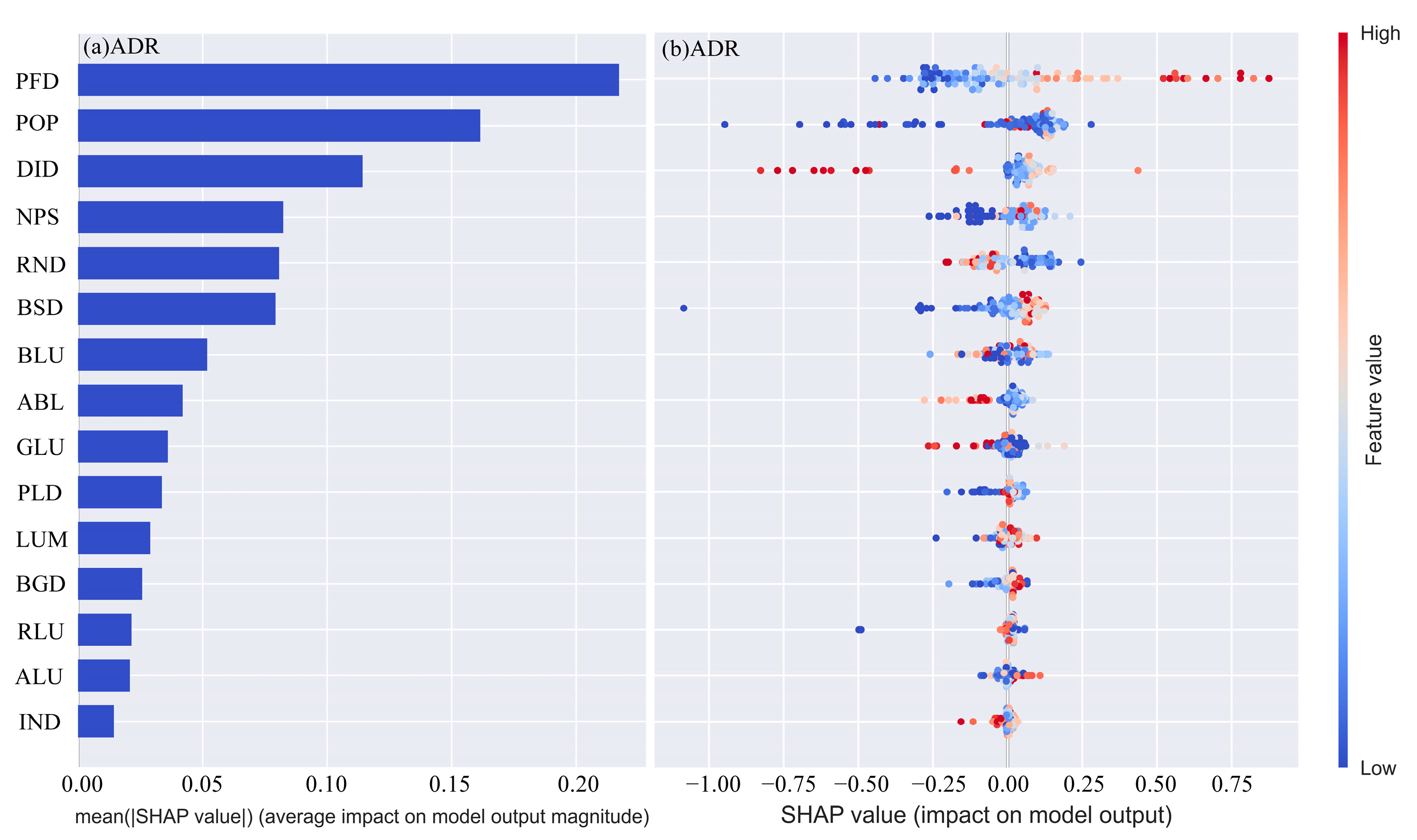
4.2.1. SHAP Variable Importance and Summary Plot

The XGBoost algorithm and SHAP method were utilized to investigate the correlation between ridership and the variables of the built environment. The importance of these variables was ranked based on the mean SHAP value, and a plot was created to visualize this ranking in descending order. Similarly, a summary plot of the SHAP values was drawn, where the y-axis represented the individual variables, the x-axis represented the SHAP values of the samples, and the colors indicated the magnitude of the variable eigenvalues. To enhance the visualization, overlapping sample points were set to jitter in the y-axis direction (Figure 3). For the average daily ridership results, the POI facility density (PFD) (mean SHAP = 0.22) and population density (POP) (mean SHAP = 0.16) emerged as the two most significant elements. Distance from downtown (DID), number of parks and squares (NPS), road network density (RND), and bus stop density (BSD) were the other important features of this study. The source and direction of ridership were associated with the development and construction of station areas, suggesting that a high-density service facility layout could enhance metro utilization. Furthermore, ridership generation was dominated by human activity, underscoring the substantial influence of the POP [6]. The importance of variables such as DID and RND has been confirmed in several studies [12,48,49]. In terms of time-varying ridership, the ranking of influential factors slightly differs, indicating that the built environment’s variables exert time-driven effects on ridership numbers, but the overall influence of PFD, parking lot density (PLD), NPS, and BSD is greater. These results also reflect the important roles of private cars and buses in the “last-mile” connection mode and prove that attractions, such as parks and squares, are important to Xi’an’s urban travel results [14]. It is noteworthy that the overall significance of the impact of land use mixture (LUM) and residential LU (RLU) is poor, which is a result that differs from previous studies conducted in Nanjing, China, and Seoul, Korea, indicating that the mix of land use and the share of residential land area were significantly positively correlated with metro ridership numbers [26,50]. The reasons for this result may include the following factors: first, the result is linked to the limited variation in mixed land use within the metro station zones in Xi’an, and second, the different development intensities of the land are also an important cause of the non-significant effect [19,51].

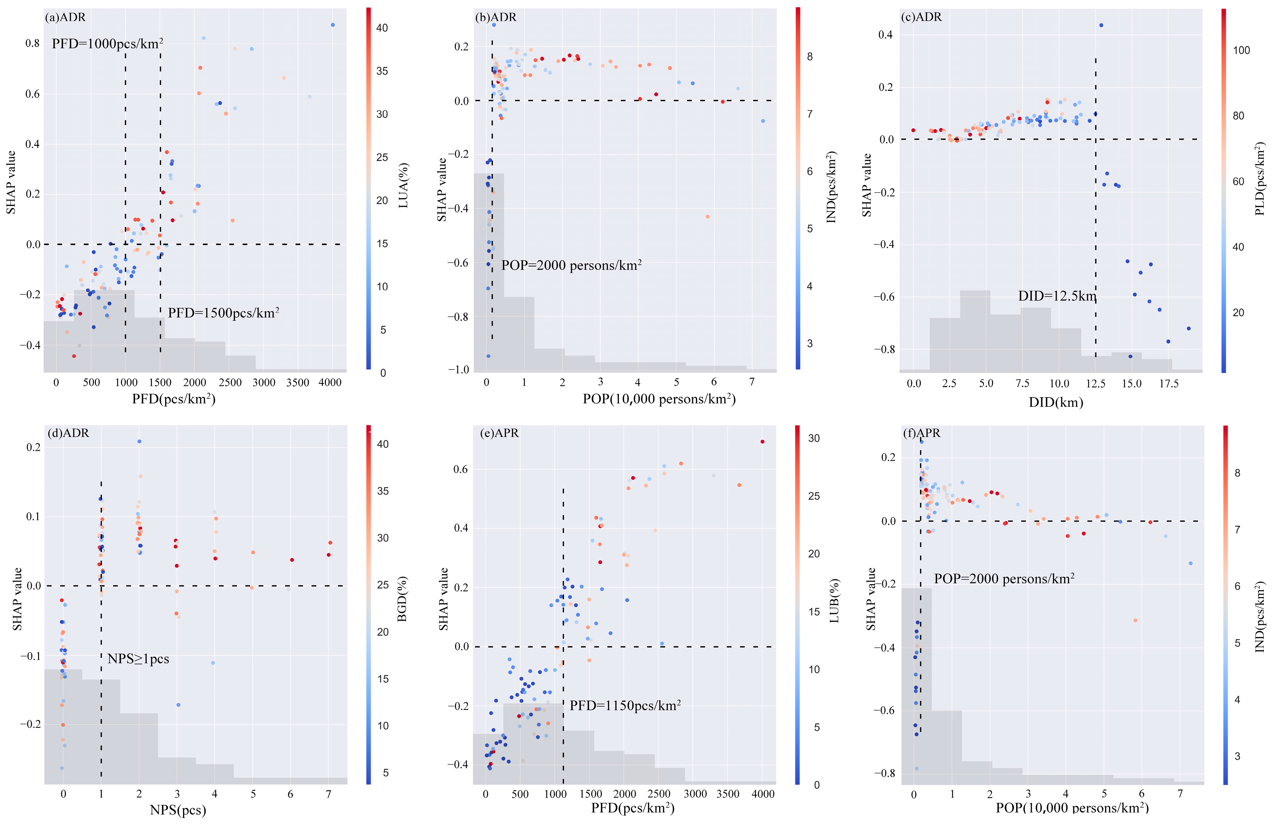
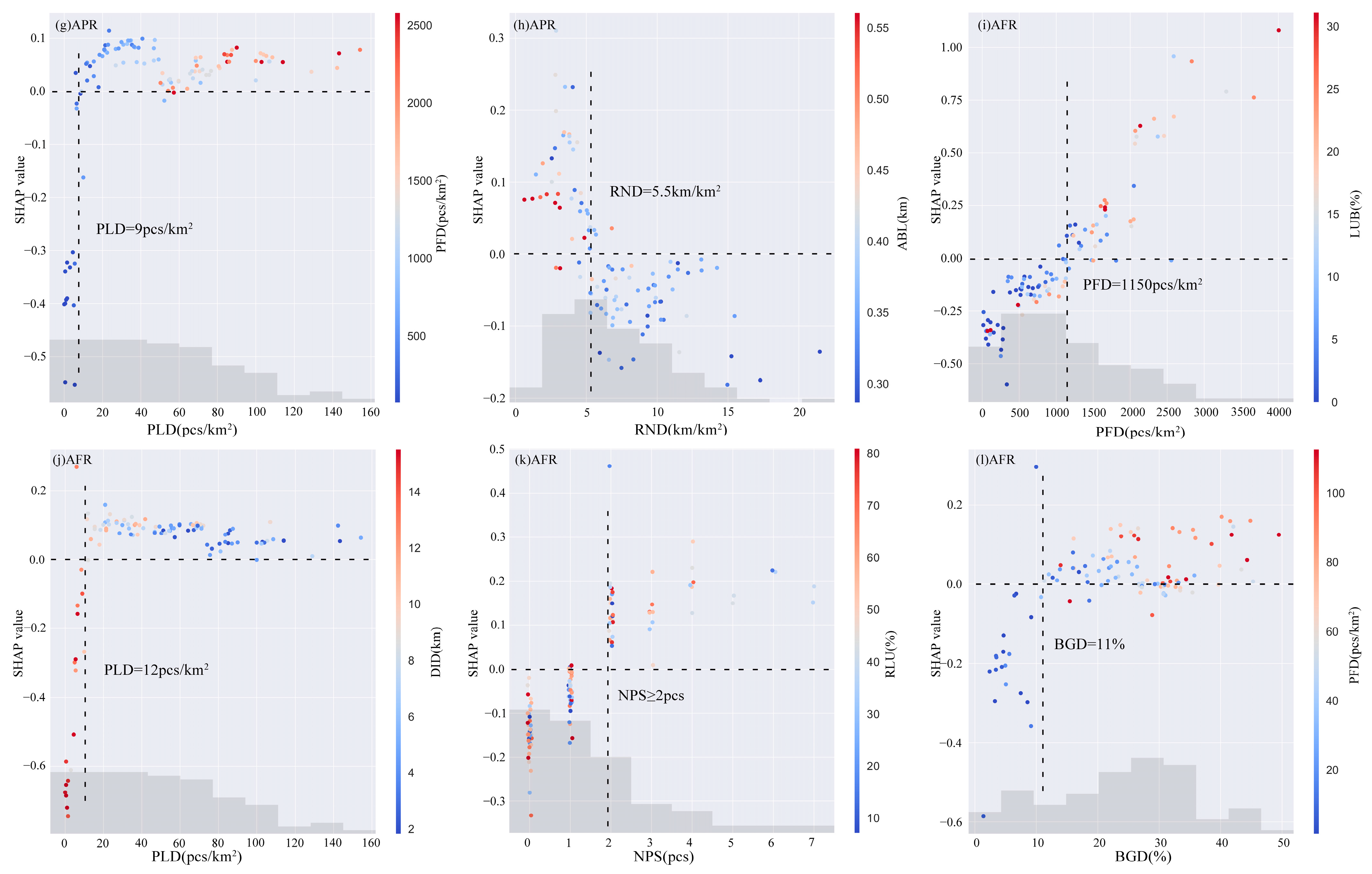
4.2.2. Nonlinear Effects of Built Environment Variables on Ridership Numbers

According to the variable importance analysis, this study selected the top four significant built environment variables from each of the three models and plotted a partial dependency graph to illustrate the nonlinear relationships (Figure 4). The bar chart represents the frequency distribution characteristics of the variable eigenvalues. The different colors indicate the magnitude of the value of another variable that interacts most strongly with that variable at each metro station.
For the PFD (Figure 4a), the SHAP value gradually increases until it reaches about 1500 pcs/km2, and the effect of this variable on the average daily ridership transitions from a negative to a positive outcome. Second, the interaction effect between the PFD and public LU (LUA) shows that a large LUA synergistically promotes ridership when the PFD is in the range of 1000~1500 pcs/km2 [52]. The PFD values of both peak hourly average ridership and flat hourly average ridership activities are 1150 pcs/km2 (Figure 4e,i), and the high occupancy of commercial LU (LUB) synergistically creates a positive effect. The reason for this outcome could be that these station types create more jobs and commercial activities, which provide more destination and activity options [10,13,53]. Therefore, the density of facilities at the site should be higher than the critical value to ensure the promotion of ridership behavior.
Figure 4b shows that the effect of the POP on the average daily ridership numbers is negative at a low value and becomes positive and stabilizes when it exceeds 2000 persons/km2. This is the result possibly because as the population of a region becomes more concentrated, more people travel by metro, but when metro ridership activity is too high or even “overloaded”, rail travel reduces, and the ridership number does not increase [19]. The effect of the POP on peak hour average ridership is similar (Figure 4f), but it shows that with an increase in the population density, the effect gradually decreases and becomes negative, which indicates that during the necessary commuting trips performed during peak hours, people choose other modes of transportation according to how they perceive the scenario to ensure that their journey is efficient.
DID = 12.5 km is the critical value of the variable (Figure 4c). This result shows that the city center attracts more people compared to other areas. The city center has complete public service facilities and concentrated jobs. To utilize various resources, such as commerce, tourism, employment, and education, most of the travelers living at the periphery of the city need to migrate to the city center over a short distance. However, as the distance between their region and the city center increases, the elevated travel time and costs become a priority, causing station ridership numbers to stabilize [41]. When the critical value is exceeded, a negative effect is evident.
Similarly, it can be observed that NPS ≥ 1 pcs (Figure 4d), PLD = 9 pcs/km2 (Figure 4g), RND = 5.5 km/km2 (Figure 4h), PLD = 12 pcs/km2 (Figure 4j), NPS ≥ 2 pcs (Figure 4k), and BGD = 11% (Figure 4l) are the critical values of the different models. The identification of these threshold values highlights the original linear model’s analysis of the drivers, and the change in values can provide clearer information regarding the issues of metro station patronage and built environment optimization and management.

4.3. Spatial Variation Effects of Built Environment Variables on Metro Ridership Numbers

To more thoroughly explore the disparities between the influence of significant variables on stations situated in various regions, this study spatially mapped local SHAP values. This allowed us to examine the spatial heterogeneity of the impact of the built environment variables on the metro ridership numbers during distinct periods. Due to spatial constraints, the local SHAP of the POP (population density), NPS (number of parks and squares), and PLD (parking lot density) were mapped, as shown in Figure 5, Figure 6 and Figure 7.
In the ADR model, the POP shows significant spatial heterogeneity (Figure 5a). Most of the positive coefficient areas are situated in the city center area, specifically distributed along Line 2 and the surrounding stations. This is because the stations located in the central area usually serve as transportation hubs, attracting a substantial number of people, logistics, and information flows, and form the activity center of the area, while the population in the fringe areas of the city, where the metro is less densely distributed, prefers to remain in the region. For long-distance activities, individuals choose to travel by car [54]. In the APR model (Figure 5b), it can be observed that the positive coefficients of the stations in the Weiyang and Yanta districts are higher, while negative impacts are mostly evident in the Baqiao district. This conclusion is reasonable because urban residents mostly need to commute to districts during peak hours, while residents living in the city center more often choose to commute short distances on foot or by bicycle [55]. At the same time, the northeastern part of the city is inadequately connected to other regions, and the increase in commuting time for long distances prompts residents to seek out workplaces closer to home. These plots also show that the peak SHAP coefficients are significantly lower than the average daily patronage, suggesting that the effect of the population distribution on patronage diminishes during peak hours.
The heterogeneous distribution of the local coefficients of the NPS in the ADR and AFR models does not show a strong pattern in space (Figure 6). The distribution of surrounding attractions is typically considered in the design of the Xi’an Metro lines. This makes the attraction of scenic spots more powerful when there are multiple, large scenic spots compared to stations with ordinary urban green spaces and small venues, and these destinations greatly contribute to the metro ridership numbers, such as those observed for Xiaozhai Station, Big Wild Goose Pagoda Station, and Convention and Exhibition Center Station. A lack of parks or squares in station areas has negative effects on ridership numbers, too. In addition, as shown in Figure 3, it can be observed that people tend to avoid visiting tourist attractions during the morning and evening peak hours to ensure a more comfortable experience and reduce their waiting times.
PLD, as a metro–motor vehicle feeder facility, has a significant spatial impact on metro ridership numbers (Figure 7). The effect is similar to that of the POP, which forms a “circle” structure, a phenomenon that can be related to the city’s transportation demand and urban planning outcomes [25,52]. As the number of parking lots increases in the central region, drivers can choose to park their cars in the parking lots and transfer to the metro due to traffic congestion, thus increasing metro ridership numbers. Another possible explanation for this activity is that parking costs are higher in the central region and people may prefer to travel by metro, which is cheaper to use [31]. In the outer circles, residents tend to rely more on surface transportation modes, and the availability of parking lots can encourage residents to use private cars to commute to work.

4.4. Metro Station Clustering and Optimization

In accordance with the differences in the spatial impact of built environment characteristics on ridership numbers, this study categorized different site types using the K-means clustering method based on the SHAP values. The sum of squared errors (SSE) was calculated to determine the optimal number of clusters for each model, and the periods at which the SSE slowly decreased and stabilized were considered to be the points of optimal clustering [5]. The optimal number of clusters was four in the ADR and AFR models and five in the APR model. The clustering outcomes of the three models varied somewhat, and the stations were classified into types with corresponding optimization suggestions based on the following criteria: (1) if a station was classified as the same type in two or more clustering results, it was assigned to that category; (2) if a station fell into different categories, it was classified by amalgamating the characteristics of ridership and the built environment. Ultimately, the stations were divided into four distinct classes (Figure 8d).
Cluster 1 included stations that were located on Line 2, which opened in 2011, or the Old Town area. The PFD coefficients of the stations in this cluster are much higher than those of the other stations (Figure 8a–c), which means that the same PFD density generates a higher ridership value for this type of station compared to other stations. This conclusion can lead planning authorities to focus on increasing the density of the facility, thereby increasing the trip-sharing rate of the metro. In fact, based on the ridership characteristics, these types of stations have extremely high ridership numbers, both during peak and flat scenarios. Therefore, promoting the flow of this type of station negatively affects the urban transportation network system. At the same time, it can be observed that the RND coefficient of this type of site has a negative impact (Figure 8b), which may be caused by the high-density road network structure in the old city area. This leads to travelers having more options, the urban functional area being more concentrated, and the cost and time of travel also being lower relative to the main street area mode, which is more conducive to the creation of an efficient, slow-moving system in the region. Part of the reason for this negative impact is that residents living in the old city area with a higher income also prefer to travel to work by private car and cabs [55]. Ultimately, this leads to a high load on both surface and underground transportation services in the vicinity of the station. Therefore, in the current urban development planning scenario, it is possible to transfer the layout of facilities related to such stations to the neighboring stations in an orderly manner, and the functions of the flow of people in the stations can be reduced so as to balance the flow of passengers at different times of the day and to reduce the wastage of metro transport resources due to an extreme flow of passengers. In addition, improving the overall efficiency of transport interchange is also a proven solution.
The Cluster 2 sites are distributed along various routes. These stations are located closer to the city center relative to the Cluster 3 and 4 stations and assume the role of easing the flow of people at the Cluster 1 stations. Increasing the PFD, POP, and PLD increases station ridership numbers when the other conditions are consistent. The results of these studies show that the abovementioned significant factors must be improved in order to alleviate the problem of a single passenger flow structure, promote the continuous improvement of urban functions in the region, increase travel destinations, and form an urban spatial structure linked by site areas. In the process of policy developments, site developments must be promptly assessed to avoid the formation of new high-load development site clusters [5].
Cluster 3 includes stations in the Weiyang, Lianhu, and Yanta districts. These areas have convenient transportation modes, and residents are characterized by their short–medium distance and strong centripetal travel activities. The coefficients of the PFD in different models show a negative effect (Figure 8a–c), which suggests that the station areas satisfy people’s various living requirements; in areas with densely packed facilities, people also have more transportation choices, which reduces the number of metro trips [56]. This is crucial for policy formulation. Secondly, the POP, DID, and PLD had positive effects. These results indicate that focusing on population density and the number of parking lots in this area is beneficial for metro ridership. Within this cluster, as the DID increased, more parking lots were added for residents, thus attracting more employment opportunities. However, it is also important to note that Line 2 runs through the old city center of Xi’an, and a single addition to the ridership number will result in an increased burden on the line. This scenario coincides with the expected plan in the Xi’an 14th Five-Year Plan for Comprehensive Transportation Development [57], where the addition of parallel alternative routes will greatly reduce the ridership pressure on Line 2.
Cluster 4 includes most stations in the Baqiao district and other marginal stations. The effects of different influencing factors on this cluster are negative, and the ridership numbers at these stations remain in a low vitality state. The essential reason for this outcome is the mismatch between the highly developed areas and low-density metro network in the region and the mismatch between the regional space and routes has resulted in more people choosing to work and move around locally, with cars becoming the main mode of travel. A reasonable increase in the line density or the use of an urban metro loop could effectively improve the connectivity of the line and accessibility of travel, reducing the travel time, for example, by constructing lines in the more densely populated areas of Baqiao district, strengthening the connection between Lines 3 and 9, and improving the travel efficiency for people living in suburban areas. On this basis, the mechanism of the relevant factors in Cluster 3 can provide reference and guidance for the next policy formulation.

5. Conclusions

In this study, the XGBoost-SHAP model was utilized to investigate the nonlinear impacts and spatial effects of “5D” built environment characteristics on the average daily, peak, and flat ridership numbers in metro station areas, and K-means clustering analysis was employed to divide the stations by combining it with local SHAP coefficients. Planning and policy recommendations were proposed based on the clustering results. The XGBoost model had better fitting and predictive power results compared to the linear model, which was a clear advantage for solving such problems. The SHAP model provided realistic and accurate estimates at the local level. The main research results are as follows.
Firstly, the built environment variable of the POI facility density has a significant nonlinear impact on metro ridership across various time frames. Different variables have time-driven and threshold effects in different models. For example, in the average daily ridership model, a POI facility density = 1500 pcs/km2, a population density = 2000 persons/km2, a distance from downtown = 12.5 km, and a number of parks and squares ≥ 1 pcs are the threshold values of the variables, and a high percentage of public LU(A) can promote ridership numbers, together with POI facility density.
Secondly, the local SHAP coefficients show the heterogeneity of the spatial impacts: population density has a positive impact on the city center area and a negative impact on other areas; the number of parks and squares presents no obvious pattern in space but reflects the important contribution of tourist attractions to the ridership numbers in Xi’an; and the effect of parking lot density is similar to that of population density, forming a “circle” structure. The effect of parking lot density is similar to that of population density, forming a “circle” structure.
Finally, K-means clustering analysis was performed based on the values of local SHAP coefficients mapped into space. According to the influence of different built environments, the sites were divided into four classes, and differentiated guidance strategies and planning objectives were proposed. For example, for the stations located at Cluster 1, the site functions were shifted to the neighboring stations to reduce the impact of high ridership activity on the metro network while considering the characteristics of ridership. Increasing the metro ridership number was not the sole aim of this study; rather, the optimization of the built environment was accurately proposed based on time, location, station area planning, and other characteristics.
This study has limitations concerning several aspects that deserve further research. On the one hand, the scope of the PCA in this study was defined as an 800 m radius, but the influence domain of the PCA could slightly differ depending on the station, and in the future, the actual service areas in different stations should be divided using big data in metro traveling research to improve the accuracy of the study. On the other hand, this study relied on spatial and temporal big data of different granularities, including multi-time travel, POI, and station built environment data. Fusion analysis of the data produced relative errors in the results. This type of problem has also been frequently observed in related studies [11,13], and in future research, it can be solved by using finer-grained big data. In addition, due to the desensitization of big data, this study ignored the social attributes of the traveling population at each station. Thus, in the future, it is necessary to combine social media location data or mobile phone signaling data to explore the effects of different attributes of the population and ridership behavior [58]. Finally, given the inconsistencies in the scale and stage of urban development in China, it remains to be seen whether the thresholds and spatial effects obtained in this study are applicable to other regions, and a larger sample size or multiple modeling approaches should be used to verify the robustness of the results in different spatial units. Multiple cities were selected for side-by-side comparisons or in-depth studies based on different machine learning algorithms.

Author Contributions

Conceptualization: Yafei Xi and Quanhua Hou. Data curation: Quanhua Hou, Yafei Xi and Yaqiong Duan. Formal analysis: Yafei Xi, Yaqiong Duan and Kexin Lei. Funding acquisition: Quanhua Hou and Yaqiong Duan. Investigation: Yan Wu. Methodology: Quanhua Hou, Yafei Xi, Yaqiong Duan and Yan Wu. Project administration: Quanhua Hou, Yaqiong Duan and Yan Wu. Resources: Quanhua Hou and Yan Wu. Software: Yafei Xi, Kexin Lei and Qianyu Cheng. Supervision: Quanhua Hou, Yaqiong Duan and Yan Wu. Validation: Quanhua Hou and Yan Wu. Visualization: Quanhua Hou and Yan Wu. Writing—original draft: Yafei Xi. All authors have read and agreed to the published version of the manuscript.

Funding

This research was supported by the Fundamental Research Funds for the Central Universities (Grant No. 300102411608), and Xi’an Social Science Planning Fund Project (Grant No. 23GL69).

Data Availability Statement

Data are contained within the article.

Acknowledgments

We are thankful to the anonymous reviewers for their valuable comments.

Conflicts of Interest

The authors declare that they have no known competing financial interests or personal relationships that could have appeared to influence the work reported in this paper.

References

  1. Hrelja, R. Cars. Problematisations, Measures and Blind Spots in Local Transport and Land Use Policy. Land Use Policy 2019, 87, 104014. [Google Scholar] [CrossRef]
  2. Nieuwenhuijsen, P.M.; Khreis, H. CAR Free Cities: Pathways to a Healthy Urban Living. J. Transp. Health 2016, 3, S26. [Google Scholar] [CrossRef]
  3. Li, Q.; Peng, J.; Yang, H. Research on Relationship Analysis between Passenger Flow Characteristics of Rail Transit Stations and Built Environment of Different Station Areas in Wuhan. J. Geo-Inf. Sci. 2021, 23, 1246–1258. [Google Scholar]
  4. Gao, D.; Xu, Q.; Chen, P.; Hu, J.; Zhu, Y. Spatial Characteristics of Urban Rail Transit Passenger Flows and Fine-Scale Built Environment. J. Transp. Syst. Eng. Inf. Technol. 2021, 21, 25–32. [Google Scholar]
  5. Li, S.; Lyu, D.; Huang, G.; Zhang, X.; Gao, F.; Chen, Y.; Liu, X. Spatially Varying Impacts of Built Environment Factors on Rail Transit Ridership at Station Level: A Case Study in Guangzhou, China. J. Transp. Geogr. 2020, 82, 102631. [Google Scholar] [CrossRef]
  6. Cardozo, O.D.; García-Palomares, J.C.; Gutiérrez, J. Application of Geographically Weighted Regression to the Direct Forecasting of Transit Ridership at Station-Level. Appl. Geogr. 2012, 34, 548–558. [Google Scholar] [CrossRef]
  7. Chen, L.; Lu, Y.; Liu, Y.; Yang, L.; Peng, M.; Liu, Y. Association between Built Environment Characteristics and Metro Usage at Station Level with a Big Data Approach. Travel Behav. Soc. 2022, 28, 38–49. [Google Scholar] [CrossRef]
  8. Chen, E.; Ye, Z.; Wang, C.; Zhang, W. Discovering the Spatio-Temporal Impacts of Built Environment on Metro Ridership Using Smart Card Data. Cities 2019, 95, 102359. [Google Scholar] [CrossRef]
  9. Choi, J.; Lee, Y.J.; Kim, T.; Sohn, K. An Analysis of Metro Ridership at the Station-to-Station Level in Seoul. Transportation 2012, 39, 705–722. [Google Scholar] [CrossRef]
  10. Zhao, J.; Deng, W.; Song, Y.; Zhu, Y. What Influences Metro Station Ridership in China? Insights from Nanjing. Cities 2013, 35, 114–124. [Google Scholar] [CrossRef]
  11. Ding, C.; Cao, X.; Liu, C. How Does the Station-Area Built Environment Influence Metrorail Ridership? Using Gradient Boosting Decision Trees to Identify Non-Linear Thresholds. J. Transp. Geogr. 2019, 77, 70–78. [Google Scholar] [CrossRef]
  12. Gan, Z.; Yang, M.; Feng, T.; Timmermans, H.J.P. Examining the Relationship between Built Environment and Metro Ridership at Station-to-Station Level. Transp. Res. D Transp. Environ. 2020, 82, 102332. [Google Scholar] [CrossRef]
  13. Shao, Q.; Zhang, W.; Cao, X.; Yang, J.; Yin, J. Threshold and Moderating Effects of Land Use on Metro Ridership in Shenzhen: Implications for TOD Planning. J. Transp. Geogr. 2020, 89, 102878. [Google Scholar] [CrossRef]
  14. Du, Q.; Zhou, Y.; Huang, Y.; Wang, Y.; Bai, L. Spatiotemporal Exploration of the Non-Linear Impacts of Accessibility on Metro Ridership. J. Transp. Geogr. 2022, 102, 103380. [Google Scholar] [CrossRef]
  15. Ma, X.; Zhang, J.; Ding, C.; Wang, Y. A Geographically and Temporally Weighted Regression Model to Explore the Spatiotemporal Influence of Built Environment on Transit Ridership. Comput. Environ. Urban Syst. 2018, 70, 113–124. [Google Scholar] [CrossRef]
  16. Zhu, H.; Peng, J.; Dai, Q.; Yang, H. Exploring the Long-Term Threshold Effects of Density and Diversity on Metro Ridership. Transp. Res. D Transp. Environ. 2024, 128, 104101. [Google Scholar] [CrossRef]
  17. Wu, P.; Xu, L.; Zhong, L.; Gao, K.; Qu, X.; Pei, M. Revealing the Determinants of the Intermodal Transfer Ratio between Metro and Bus Systems Considering Spatial Variations. J. Transp. Geogr. 2022, 104, 103415. [Google Scholar] [CrossRef]
  18. Cervero, R.; Murakami, J.; Miller, M. Direct Ridership Model of Bus Rapid Transit in Los Angeles County, California. Transp. Res. Rec. J. Transp. Res. Board 2010, 2145, 1–7. [Google Scholar] [CrossRef]
  19. Lei, K.; Hou, Q.; Li, W.; Zhao, M.; Zhou, J.; Zhang, L.; Chen, S.; Duan, Y. The Impact of Land Use on Time-Varying Passenger Flow Based on Site Classification. Land 2022, 11, 2189. [Google Scholar] [CrossRef]
  20. Sung, H.; Oh, J.-T. Transit-Oriented Development in a High-Density City: Identifying Its Association with Transit Ridership in Seoul, Korea. Cities 2011, 28, 70–82. [Google Scholar] [CrossRef]
  21. Wang, D.; Chai, Y.; Li, F. Built Environment Diversities and Activity–Travel Behaviour Variations in Beijing, China. J. Transp. Geogr. 2011, 19, 1173–1186. [Google Scholar] [CrossRef]
  22. Cervero, R. Built Environments and Mode Choice: Toward a Normative Framework. Transp. Res. D Transp. Environ. 2002, 7, 265–284. [Google Scholar] [CrossRef]
  23. Ewing, R.; Cervero, R. Travel and the Built Environment. J. Am. Plan. Assoc. 2010, 76, 265–294. [Google Scholar] [CrossRef]
  24. Moniruzzaman, M.; Páez, A. Accessibility to Transit, by Transit, and Mode Share: Application of a Logistic Model with Spatial Filters. J. Transp. Geogr. 2012, 24, 198–205. [Google Scholar] [CrossRef]
  25. Durning, M.; Townsend, C. Direct Ridership Model of Rail Rapid Transit Systems in Canada. Transp. Res. Rec. J. Transp. Res. Board 2015, 2537, 96–102. [Google Scholar] [CrossRef]
  26. Jun, M.-J.; Choi, K.; Jeong, J.-E.; Kwon, K.-H.; Kim, H.-J. Land Use Characteristics of Subway Catchment Areas and Their Influence on Subway Ridership in Seoul. J. Transp. Geogr. 2015, 48, 30–40. [Google Scholar] [CrossRef]
  27. An, D.; Tong, X.; Liu, K.; Chan, E.H.W. Understanding the Impact of Built Environment on Metro Ridership Using Open Source in Shanghai. Cities 2019, 93, 177–187. [Google Scholar] [CrossRef]
  28. Li, S.; Lyu, D.; Liu, X.; Tan, Z.; Gao, F.; Huang, G.; Wu, Z. The Varying Patterns of Rail Transit Ridership and Their Relationships with Fine-Scale Built Environment Factors: Big Data Analytics from Guangzhou. Cities 2020, 99, 102580. [Google Scholar] [CrossRef]
  29. Liu, X.; Chen, X.; Potoglou, D.; Tian, M.; Fu, Y. Travel Impedance, the Built Environment, and Customized-Bus Ridership: A Stop-to-Stop Level Analysis. Transp. Res. D Transp. Environ. 2023, 122, 103889. [Google Scholar] [CrossRef]
  30. Yang, H.; Xu, T.; Chen, D.; Yang, H.; Pu, L. Direct Modeling of Subway Ridership at the Station Level: A Study Based on Mixed Geographically Weighted Regression. Can. J. Civ. Eng. 2020, 47, 534–545. [Google Scholar] [CrossRef]
  31. Wang, Z.; Song, J.; Zhang, Y.; Li, S.; Jia, J.; Song, C. Spatial Heterogeneity Analysis for Influencing Factors of Outbound Ridership of Subway Stations Considering the Optimal Scale Range of “7D” Built Environments. Sustainability 2022, 14, 16314. [Google Scholar] [CrossRef]
  32. Lundberg, S.; Lee, S.-I. A Unified Approach to Interpreting Model Predictions. In NIPS’17: Proceedings of the 31st International Conference on Neural Information Processing Systems, Long Beach, CA, USA, 4–9 December 2017; Curran Associates Inc.: Red Hook, NY, USA, 2017; pp. 4768–4777. [Google Scholar]
  33. Guo, T.; Liu, B.; Tian, L.; Sun, A. Research on TOD Reasonable Area around Urban Rail Traffic Site—A Case Study of West Jiangnan Station on Guangzhou No.2 Subway Line. Planners 2008, 24, 75–78. [Google Scholar]
  34. Zhao, M.; Tong, H.; Li, B.; Duan, Y.; Li, Y.; Wang, J.; Lei, K. Analysis of Land Use Optimization of Metro Station Areas Based on Two-Way Balanced Ridership in Xi’an. Land 2022, 11, 1124. [Google Scholar] [CrossRef]
  35. Gan, Z.; Yang, M.; Feng, T.; Timmermans, H. Understanding Urban Mobility Patterns from a Spatiotemporal Perspective: Daily Ridership Profiles of Metro Stations. Transportation 2020, 47, 315–336. [Google Scholar] [CrossRef]
  36. Cervero, R.; Kang, C.D. Bus Rapid Transit Impacts on Land Uses and Land Values in Seoul, Korea. Transp. Policy 2011, 18, 102–116. [Google Scholar] [CrossRef]
  37. Zhang, H. Extracting Active Population Data Based on Baidu Heat Maps for Transportation Planning Applications. Urban Transp. China 2021, 19, 103–111. [Google Scholar]
  38. Park, K.; Ewing, R.; Scheer, B.C.; Tian, G. The Impacts of Built Environment Characteristics of Rail Station Areas on Household Travel Behavior. Cities 2018, 74, 277–283. [Google Scholar] [CrossRef]
  39. Xi, Y.; Hou, Q.; Duan, Y.; Lei, K.; Wu, Y.; Cheng, Q. Nonlinear Relationships between Built Environmental Characteristics and Ridership in Xi’an Metro Station. 6 July 2023, Preprint (Version 1). Available at Research Square. Available online: https://www.researchsquare.com/article/rs-3134638/v1 (accessed on 10 November 2023).
  40. Chen, T.; Guestrin, C. XGBoost. In Proceedings of the 22nd ACM SIGKDD International Conference on Knowledge Discovery and Data Mining, San Francisco, CA, USA, 13–17 August 2016; ACM: New York, NY, USA, 2016; pp. 785–794. [Google Scholar]
  41. Ding, C.; Cao, X.; Næss, P. Applying Gradient Boosting Decision Trees to Examine Non-Linear Effects of the Built Environment on Driving Distance in Oslo. Transp. Res. Part A Policy Pract. 2018, 110, 107–117. [Google Scholar] [CrossRef]
  42. Fu, C.; Huang, Z.; Scheuer, B.; Lin, J.; Zhang, Y. Integration of Dockless Bike-Sharing and Metro: Prediction and Explanation at Origin-Destination Level. Sustain. Cities Soc. 2023, 99, 104906. [Google Scholar] [CrossRef]
  43. Shapley, L. A Value for N-Person Games; RAND Corporation: Santa Monica, CA, USA, 1952. [Google Scholar]
  44. Barua, L.; Zou, B.; Zhou, Y.; Liu, Y. Modeling Household Online Shopping Demand in the U.S.: A Machine Learning Approach and Comparative Investigation between 2009 and 2017. Transportation 2023, 50, 437–476. [Google Scholar] [CrossRef] [PubMed]
  45. Yuan, C.; Yang, H. Research on K-Value Selection Method of K-Means Clustering Algorithm. J 2019, 2, 226–235. [Google Scholar] [CrossRef]
  46. Liu, X.; Chen, X.; Tian, M. Effects of Built Environment on Metro Ridership Considering Stage of Growth. J. Transp. Syst. Eng. Inf. Technol. 2023, 23, 121–127. [Google Scholar]
  47. Liu, M.; Liu, Y.; Ye, Y. Nonlinear Effects of Built Environment Features on Metro Ridership: An Integrated Exploration with Machine Learning Considering Spatial Heterogeneity. Sustain. Cities Soc. 2023, 95, 104613. [Google Scholar] [CrossRef]
  48. Liu, C.; Erdogan, S.; Ma, T.; Ducca, F.W. How to Increase Rail Ridership in Maryland: Direct Ridership Models for Policy Guidance. J. Urban Plan. Dev. 2016, 142, 04016017. [Google Scholar] [CrossRef]
  49. Yu Li, X.; Krishna Sinniah, G.; Li, R. Identify Impacting Factor for Urban Rail Ridership from Built Environment Spatial Heterogeneity. Case Stud. Transp. Policy 2022, 10, 1159–1171. [Google Scholar] [CrossRef]
  50. Shi, Z.; Zhang, N.; Liu, Y.; Xu, W. Exploring Spatiotemporal Variation in Hourly Metro Ridership at Station Level: The Influence of Built Environment and Topological Structure. Sustainability 2018, 10, 4564. [Google Scholar] [CrossRef]
  51. Li, J.; Yao, M.; Ji, F.; Xiang, L. Quantitative Study on How Land Use Mix Impact Urban Rail Transit at Station-Level. J. Tongji Univ. (Nat. Sci.) 2016, 44, 1415–1423. [Google Scholar]
  52. Kuby, M.; Barranda, A.; Upchurch, C. Factors Influencing Light-Rail Station Boardings in the United States. Transp. Res. Part A Policy Pract. 2004, 38, 223–247. [Google Scholar] [CrossRef]
  53. Loo, B.P.Y.; Chen, C.; Chan, E.T.H. Rail-Based Transit-Oriented Development: Lessons from New York City and Hong Kong. Landsc. Urban Plan. 2010, 97, 202–212. [Google Scholar] [CrossRef]
  54. Fu, X.; Zhao, X.; Li, C.; Cui, M.; Wang, J.; Qiang, Y. Exploration of the Spatiotemporal Heterogeneity of Metro Ridership Prompted by Built Environment: A Multi-source Fusion Perspective. IET Intell. Transp. Syst. 2022, 16, 1455–1470. [Google Scholar] [CrossRef]
  55. Wang, J.; Wan, F.; Dong, C.; Yin, C.; Chen, X. Spatiotemporal Effects of Built Environment Factors on Varying Rail Transit Station Ridership Patterns. J. Transp. Geogr. 2023, 109, 103597. [Google Scholar] [CrossRef]
  56. Boarnet, M.; Crane, R.C. Travel by Design; Oxford University Press: Oxford, UK, 2001; ISBN 9780195123951. [Google Scholar]
  57. Xi’an Municipal People’s Government Notice of the Xi’an Municipal People’s Government on Printing and Distributing the “14th Five-Year Plan” Comprehensive Transportation Development Plan. Gazette of Xi’an Municipal People’s Government, 28 October 2021.
  58. Zhang, X.; Gao, F.; Liao, S.; Zhou, F.; Cai, G.; Li, S. Portraying Citizens’ Occupations and Assessing Urban Occupation Mixture with Mobile Phone Data: A Novel Spatiotemporal Analytical Framework. ISPRS Int. J. Geoinf. 2021, 10, 392. [Google Scholar] [CrossRef]
Figure 1. Study area.
Ijgi 13 00105 g001
Figure 2. Distribution of metro traffic by time of day.
Ijgi 13 00105 g002
Figure 3. Ranking and summary plots of features based on SHAP analysis in different models (a,c,e). Ranking of features based on average SHAP values (b,d,f). Summary plots based on range of feature values.
Ijgi 13 00105 g003aIjgi 13 00105 g003b
Figure 4. Partial dependency diagram of key variables. (ad) Partial dependency diagram of key variables in the average daily ridership(eh) Partial dependency diagram of key variables in the average peak ridership (il) Partial dependency diagram of key variables in the average flat ridership.
Ijgi 13 00105 g004aIjgi 13 00105 g004b
Figure 5. Localized coefficients of population density (POP) in average daily (ADR) and peak ridership (APR) models.
Ijgi 13 00105 g005
Figure 6. Localized coefficients of number of parks and squares (NPS) in average daily (ADR) and flat ridership (AFR) models.
Ijgi 13 00105 g006
Figure 7. Localized coefficients of parking lot density (PLD) in average peak (ADR) and flat ridership (APR) models.
Ijgi 13 00105 g007
Figure 8. Clustering results for metro stations.
Ijgi 13 00105 g008
Table 1. Model variable settings.
CategoryNameAbbr.Computational Method and InterpretationMeanStd. Deviation
Dependent variable
Average daily ridershipADRThe sum of the average daily inbound and outbound ridership in each metro station (persons)30,77722,420
Average peak ridershipAPRThe ratio of inbound and outbound ridership to the time period at the morning peak (7:00–10:00) and evening peak (17:00–20:00) (persons)26631717
Average flat ridershipAFRThe ratio of inbound and outbound ridership to the time period at times other than peak hours (persons)12261038
Independent variable
DensityBuilding densityBGDThe ratio of the building base area within the PCA of each metro station (%)23.5211.72
Population densityPOPThe ratio of the population within the PCA of each metro station calculated based on Baidu thermodynamic diagram data (10,000 persons/km2)1.151.62
DiversityLand use mixtureLUM L a n d   u s e = i = 1 k P k i ln ( P k i ) , where k denotes the number of land use classes in the station i area and Pki denotes the area proportion of class k land within the PCA of each metro station1.010.09
Residential LU (R)RLUThe ratio of residential land area within the PCA of each metro station (%)45.3321.96
Public LU (A)ALUThe ratio of land area for public administration and service facilities within the PCA of each metro station (%)17.1415.25
Commercial LU (B)BLUThe ratio of land area for commercial service facilities within the PCA of each metro station (%)11.2512.66
Green space and square LU (G)GLUThe ratio of land area for greening and squares within the PCA of each metro station (%)5.027.04
DesignRoad network densityRNDThe ratio of total road network length within the PCA of each metro station (km/km2)6.903.79
Intersection densityINDThe ratio of intersection quantity within the PCA of each metro station (pcs/km2)5.561.90
Average block side lengthABLAverage block side length within the PCA of each metro station (km)0.380.09
Parking lot densityPLDThe ratio of parking lot quantity within the PCA of each metro station (pcs/km2)50.1637.02
Bus stop densityBSDThe ratio of bus stop quantity within the PCA of each metro station (pcs/km2)4.441.92
POI facility densityPFDThe ratio of the quantity of various facilities within the PCA of each metro station (pcs/km2)1103826
DestinationNumber of parks and squaresNPSQuantity of parks and squares within the PCA of each metro station (pcs)1.481.61
Number of commercial facilitiesNCFQuantity of commercial facilities within the PCA of each metro station (pcs)888718
DistanceDistance from downtownDIDThe straight-line distance between metro station and downtown centroid point (Bell Tower) (km)7.494.21
Table 2. Comparison of model performance.
ADRAPRAFR
RMSEMAER2RMSEMAER2RMSEMAER2
OLS16923.4111160.370.511250.81819.170.55817.31497.290.47
XGBoost10357.088169.300.78714.17589.150.80342.99278.810.79
improve (%)38.80↓26.80↓52.94↑42.90↓28.08↓45.46↑58.03↓43.93↓68.09↑
Disclaimer/Publisher’s Note: The statements, opinions and data contained in all publications are solely those of the individual author(s) and contributor(s) and not of MDPI and/or the editor(s). MDPI and/or the editor(s) disclaim responsibility for any injury to people or property resulting from any ideas, methods, instructions or products referred to in the content.

