Article

Enhancing Indoor Air Quality Estimation: A Spatially Aware Interpolation Scheme

1
Electronics and Telecommunications Research Institute, Daejeon 34129, Republic of Korea
2
Department of Computer Science and Engineering, Chungnam National University, Daejeon 34134, Republic of Korea
3
Department of Software Convergence Engineering, Mokpo National University, Mokpo 58554, Republic of Korea
*
Author to whom correspondence should be addressed.
ISPRS Int. J. Geo-Inf. 2023, 12(8), 347; https://doi.org/10.3390/ijgi12080347
Submission received: 8 June 2023 / Revised: 1 August 2023 / Accepted: 16 August 2023 / Published: 18 August 2023
(This article belongs to the Topic Urban Sensing Technologies)

Abstract

:
The comprehensive and accurate assessment of the indoor air quality (IAQ) in large spaces, such as offices or multipurpose facilities, is essential for IAQ management. It is widely recognized that various IAQ factors affect the well-being, health, and productivity of indoor occupants. In indoor environments, it is important to assess the IAQ in places where it is difficult to install sensors due to space constraints. Spatial interpolation is a technique that uses sample values of known points to predict the values of other unknown points. Unlike in outdoor environments, spatial interpolation is difficult in large indoor spaces due to various constraints, such as being separated into rooms by walls or having facilities such as air conditioners or heaters installed. Therefore, it is necessary to identify independent or related regions in indoor spaces and to utilize them for spatial interpolation. In this paper, we propose a spatial interpolation technique that groups points with similar characteristics in indoor spaces and utilizes the characteristics of these groups for spatial interpolation. We integrated the IAQ data collected from multiple locations within an office space and subsequently conducted a comparative experiment to assess the accuracy of our proposed method in comparison to commonly used approaches, such as inverse distance weighting (IDW), kriging, natural neighbor interpolation, and the radial basis function (RBF). Additionally, we performed experiments using the publicly available Intel Lab dataset. The experimental results demonstrate that our proposed scheme outperformed the existing methods. The experimental results show that the proposed method was able to obtain better predictions by reflecting the characteristics of regions with similar characteristics within the indoor space.

1. Introduction

People spend the majority of their time indoors, accounting for roughly 90% of the day, which has led to a growing interest in the energy efficiency, indoor air quality (IAQ), and user comfort of buildings [1]. It is widely recognized that various IAQ factors affect the well-being, health, and productivity of indoor occupants [2,3]. The effective monitoring and a comprehensive understanding of the IAQ of indoor spaces are essential for an energy-saving design and for improving human comfort. There is active research on techniques to effectively monitor and manage the IAQ utilizing IoT technologies as well as on the impact of the IAQ on the health of indoor occupants [4,5,6,7,8,9].
Spatial interpolation is a technique that uses sample values from a known location to predict values from another unknown location. This is achieved by collecting information about the environment using sensors or other data sources and then using statistical, deterministic, or machine learning techniques to estimate the value of a variable at another location [10,11,12,13]. Accurately assessing IAQ parameters, such as temperature, humidity, CO2 concentration, and particulate matter (PM), is critical to optimizing energy use in these environments as well as maintaining occupant health and comfort [14]. The application of spatial interpolation techniques has important implications for IAQ management because this can inform the optimization of ventilation and air conditioning systems, reduce energy consumption, and maintain a healthy indoor environment for occupants. Therefore, identifying important IAQ parameters in indoor spaces and developing accurate measurement techniques and data analysis methods have become active research areas.
For large indoor spaces, such as offices, smart buildings, smart factories, schools, etc., there is a limit on the number of IAQ sensors that can be installed in the indoor space due to space constraints or financial limitations [14]. In addition, large indoor spaces are often divided into multiple rooms by walls or have other constraints, such as the presence of equipment such as air conditioners, heaters, and other structures [15,16].
Choi [17] proposed a spatial interpolation method to improve the accuracy of PM estimation based on a weighted correction according to the known importance of each point. Kaligambe [18] used an extreme gradient boosting (XGBoost) model to estimate the unmeasured room temperature, humidity, and CO2 concentrations using a limited number of sensors in a three-story smart building in Japan. Zhou [19] proposed a cross-sample learning algorithm to obtain a spatial graph model of sensors based on the horizontal and vertical effects of gravity on humidity and used it to learn the coefficient elements of labeled locations to predict the state of unlabeled locations. Machine-learning-based methods are relatively data-intensive and have a high calculation cost [20]. Choi [14] developed an accurate IAQ distribution map for large spaces using spatial interpolation methods. In their study, 18 sensors were installed in a library’s reading room, with 14 for data collection. Their study identified the optimal spatial interpolation method for each IAQ factor, determined the ideal number and layout of sensors, and confirmed the map’s effectiveness. In Huang [21], a study was conducted to select the optimal sensor installation location under the constraints of an indoor space. Their study compared two sampling methods in indoor air distribution measurement: the gridded method and the slope-based method. The data collected through each method were interpolated using the usual kriging method. As a result, the slope-based sampling method had a smaller interpolation error than the gridded method, and the authors recommended the slope-based sampling method for indoor air distribution measurement.
Spatial interpolation in indoor environments must carefully consider the spatial structure of the environment, the distance between the data points, and the characteristics of the IAQ data. Spatial structures, such as walls or equipment such as air conditioners, can introduce a significant spatial variation in these parameters, especially in large spaces. Therefore, when interpolating data from unmeasured points using data obtained from IAQ sensors installed in indoor environments, it is necessary to consider both the spatial constraints and the distance between the unmeasured point and the other data points.
Due to spatial constraints, sensors installed within an indoor space may be grouped together where there is a high degree of data correlation between them. Sensors that are highly correlated with each other can be thought of as having a high degree of similarity between the data collected from each sensor. When spatial interpolation is performed, it is possible to predict more accurate values by referring to the data of points with high similarity to the point to be predicted and utilizing these data for spatial interpolation. In this paper, we propose a spatial interpolation technique that groups points with similar characteristics in an indoor space and utilizes the characteristics of these groups for spatial interpolation.

2. Related Works

There are several techniques that are commonly used for spatial interpolation, including inverse distance weighting (IDW), kriging, natural neighbor interpolation, and the radial basis function (RBF). These methods have been used primarily for outdoor air quality interpolation, and there is little research on IAQ interpolation considering complex indoor spaces.
IDW is a simple interpolation method that uses a weighted average of the values of the nearest data points to interpolate the values at new locations [4]. The weights are determined by the inverse of the distances between the new locations and the data points. The closer a data point is to the new location, the higher its weight will be. IDW is a fast and easy-to-implement method, but it can provide inaccurate results when the data have a strong spatial structure, as it does not take into account the spatial autocorrelation of the data [22,23,24,25,26].
Kriging is a geostatistical interpolation method that uses spatial autocorrelation to interpolate the values at new locations based on the values of nearby data points [27]. The method takes into account the spatial variability of the data and uses a weighted average of the values of the nearest data points to interpolate the values at new locations [28,29,30,31]. The weights are determined by the spatial autocorrelation structure of the data, which describes how the values at different locations are related to each other. Kriging is a popular method for spatial interpolation, as it can provide accurate results, especially when the data have a strong spatial correlation [25,32,33].
Natural neighbor interpolation is a spatial interpolation method developed by Robin Sibson [34]. It is based on the Voronoi tessellation of a set of discrete spatial points. The method uses a weighted average of the values of the nearest data points to interpolate the values at new locations. The weights are determined based on the geometric relationship between the data points and the new locations, taking into account the shapes and sizes of the data clusters. Natural neighbor interpolation is beneficial when there is a high density of measured values and is particularly reliable in cases where there is limited information on the distribution of these values [35,36,37,38,39,40]. However, since natural neighbor interpolation relies on using Thiessen polygons to estimate values within corners, it is not possible to interpolate beyond the range of the measured values [14].
RBF interpolation is a method that uses radial basis functions to approximate the unknown values at new locations [41]. By using radial basis functions, it became possible to deal with higher dimensional problems in a that is way similar to dealing with two- and three-dimensional problems [42,43,44]. RBF interpolation can provide accurate results and is computationally efficient, but it can be sensitive to the choice of the radial basis functions and the parameters used in the interpolation process [45].

3. Basic Concepts

All the locations in the space of interest are referred to as points. A point is considered to be a data point if a sensor is installed to measure a value at that specific location. Points that do not have associated data sensors are referred to as unmeasured points. A specific point for which a value is to be predicted is defined as a query point. We denote the Euclidean distance between two points, p and q, as d(p, q).
A set that contains one or more points is referred to as a group. Given a group g that contains points p1, …, pn, we define the group distance GD(g) of group g as follows in Equation (1).
G D g = max p i , p j d ( p i ,   p j ) ,           i ,   j = 1 , , n
The group distance of a group is the maximum distance between any two points within the group.
Let G(p) denote the group containing point p. The virtual distance VD(p, q) between two points, p and q, is defined as follows in Equation (2).
V D p ,   q = d p ,   q ,                         w h e r e   G p = G q   d p , q + G D G ( p ) ,         w h e r e   G p G q
The virtual distance can be regarded as a measure of the distance between two points that reflects the group information.

4. Indoor Spatial Interpolation Scheme

We propose a spatial interpolation scheme that leverages the spatial constraints inherent to indoor environments. Figure 1 shows the flow chart of the proposed spatial interpolation scheme.
The proposed scheme consists of two stages: a preprocessing stage and an interpolation stage. In the first preprocessing stage, groups are assigned to all the points in the indoor space through the group clustering algorithm and the group assignment algorithm. The second interpolation step uses the group assignment information obtained in the preprocessing step, the query point, and the data values of each data point to predict the value of the query point. In the interpolation step, the group assignment information obtained in the preprocessing step is used to select the nearest neighbors to reference during interpolation, and the prediction is calculated based on the virtual distance between the query point and each nearest neighbor.

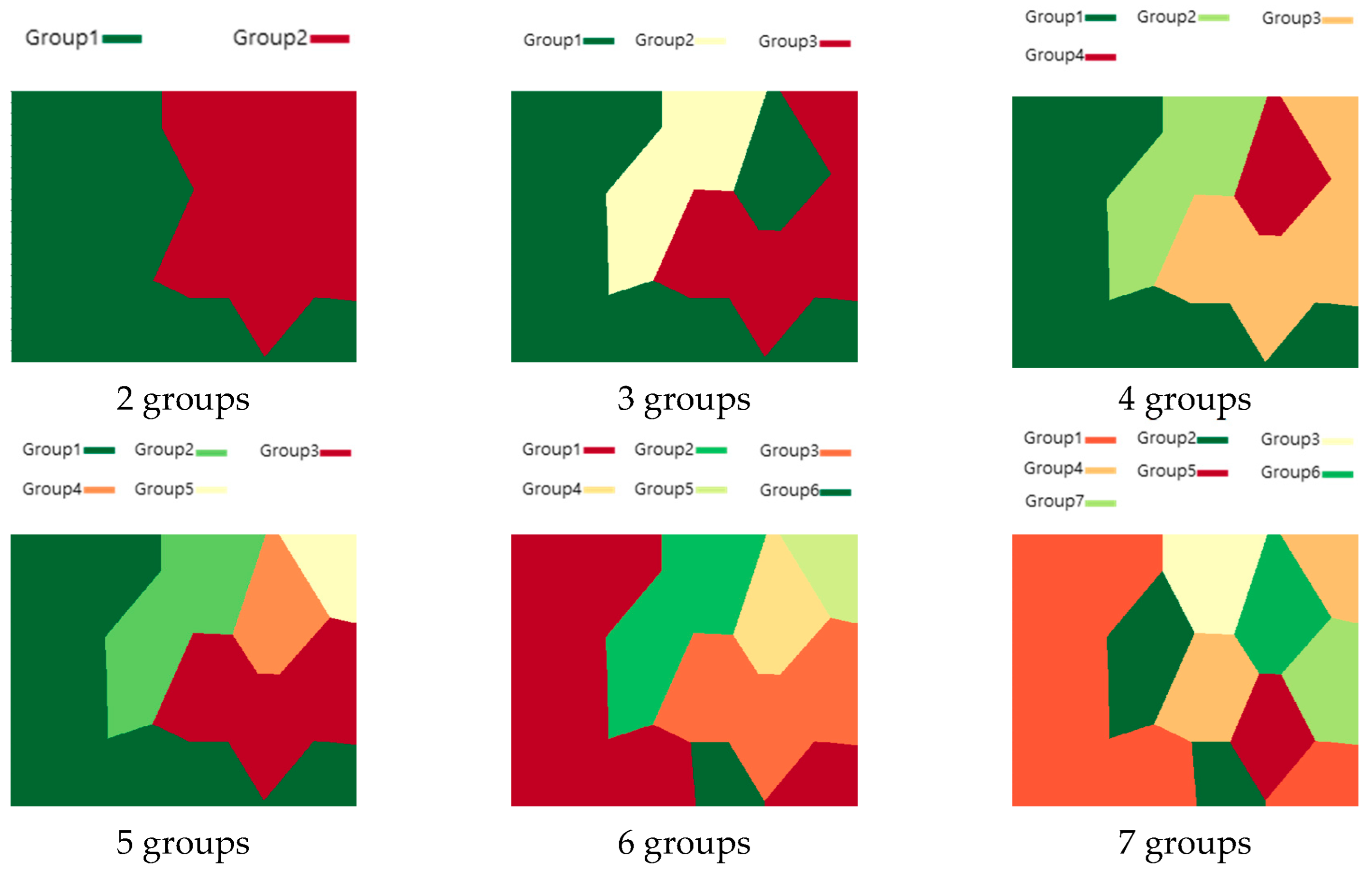
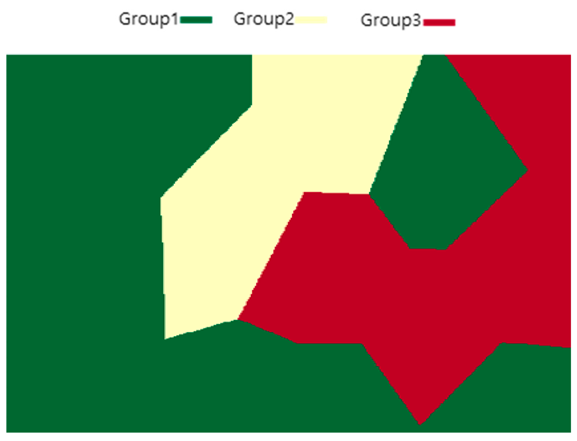
4.1. Group Clustering

Clustering is a popular technique used in unsupervised machine learning to group similar data points together. K-means is a widely used clustering algorithm that partitions a set of objects into k clusters such that the within-cluster sum of squared distances (also known as the within-group sum of squared errors, or WGSS) is minimized [46,47].
The K-mode clustering algorithm is a partitional clustering algorithm that aims to minimize the sum of the dissimilarity between data points and their assigned cluster modes [48]. The K-mode clustering algorithm is a variation of the K-means algorithm that is suitable for categorical data. The algorithm starts by randomly selecting K initial cluster modes, which are vectors that represent the mode of each categorical variable in the cluster. The distance between a data point and a cluster mode is measured using the Hamming distance, which is defined as the number of variables that differ between the two vectors. The K-means algorithm selects a centroid, which can be a virtual data point that may not correspond to any actual data point in the dataset. In contrast to K-means, the K-mode algorithm selects one of the data points in the cluster as the centroid. This is achieved by finding the mode, which is the most common value, of each of the categorical variables in the cluster.
Group clustering is defined as the process of partitioning all the data points within an indoor space into multiple clusters with the objective of ensuring that each cluster comprises points that exhibit similar spatial characteristics. The objective of group clustering is to create homogeneous groups in which the points within each group have characteristics that are more similar to each other than to the points in other groups. In this paper, the K-mode clustering algorithm is used to cluster data points. This is because the K-means algorithm may select a centroid that does not correspond to an actual data point in the dataset, whereas the K-mode algorithm always selects one of the actual data points in the cluster as the centroid. Assuming that data values collected from data points with similar spatial characteristics have similar values, this paper uses the mean squared difference (MSD) as a dissimilarity measure for the K-mode clustering algorithm. Assuming that n data points p1, , pn are given and that each data point pi has m data values, yi1, … yim for i = 1, , n. The MSD for two data points pi and pj is defined as follows in Equation (3).
M S D p i ,     p j = 1 m k = 1 m y i k y j k 2 .

4.2. Group Assignment

Group assignment refers to the process of assigning each unmeasured point in an indoor space to one of the groups created during the group clustering process. For every unmeasured point, the process involves identifying the nearest data point and assigning the same group as that of the found data point to the unmeasured point. By carrying out the group assignment process, each data point in the indoor space is assigned to a specific group. Algorithm 1 outlines the algorithm for the group assignment process.
Algorithm 1. Assign a group to an unmeasured point
procedure Group Assignment (q: unmeasured point)
 Let p1, , pn be all the data points in an indoor space
   p = argmin p i d ( p i ,   q ) ,           i = 1 , , n
G(q) = G(p)
end procedure

4.3. Group-Preferred K-Nearest Neighbor (GPKNN)

Let q be a query point and n be the number of all the data points in the same group as q. The proposed group-preferred K-nearest neighbor algorithm prioritizes data points belonging to the same group as q in contrast to the K-nearest neighbor (KNN) algorithm for q, which simply finds the K nearest data points. This group-preferred algorithm identifies K data points with a smaller virtual distance from q. Replacing the Euclidean distance function in the K-nearest neighbor algorithm with the virtual distance function proposed in this paper yields results equivalent to those of the group’s preferred K-nearest neighbor algorithm. Algorithm 2 presents the group-preferred K-nearest neighbor algorithm.
Algorithm 2. Find group-preferred K nearest neighbors
procedure GPKNN (q: query point, K: integer)
 Let DPSet = {p1, , pn} be a set of all the data points in an indoor space
TSet = DPSet
KSet = {}
while size(KSet) != K and TSet != {}
p = argmin p i V D ( p i ,   q ) ,         p i T S e t K S e t = K S e t   { p } T S e t = T S e t { p }
end while
return KSet
end procedure

4.4. Spatial Interpolation

We propose two types of indoor spatial interpolation methods modified from the existing IDW and kriging algorithms.

4.4.1. Spatial Structure IDW (SSI) Method

The SSI method modifies IDW to consider the spatial constraints of the indoor environments. IDW is one of the most widely used deterministic interpolation techniques. This method assumes that values measured at closer distances have a greater weight than values measured at greater distances. Since the influence of a known value is inversely proportional to its distance from an unknown data point, this method gives greater weight to the values closest to the predicted location, with the weight decreasing with distance [10]. Let q be a given query point in an indoor space. IDW estimates the data value of the given query point as a weighted sum of the data values measured at the surrounding data points as in Equation (4) [17].
y ^ q = i = 1 K w i y p i ,
where K is the number of data points used for the estimation, pi is the data point that is the i-th nearest data point to q, y(pi) is the measured value at pi, ωi is the weight value assigned to y(pi), and ŷ(q) is the estimated value at q. This method selects neighboring data points close to the query point and gives greater weight to the measured values of the points closer to the query point. Let λ(p, q) be the inverse of d(p, q) as in Equation (5) [17].
λ p , q = 1 d p , q ,
The weights of the IDW method are computed using Equation (6) [17].
w i = λ q , p i j = 1 K λ q , p j ,     i = 1 ,   ,   K ,
The SSI method uses Equation (7) to compute the weights of the selected K points.
w i = μ q , p i j = 1 K μ q , p j ,     i = 1 ,   ,   K ,
where μ(p, q) is defined as the inverse of the virtual distance between p and q as shown in Equation (8).
μ p ,   q = 1 V D ( p ,   q ) ,
The IDW method utilizes a weighted average of the measurements of closer data points to estimate the value at a query point. The weights are determined by the reciprocal of the distance between the query point and the data points. Data points that are closer to the query point have higher weights. The SSI method calculates weights using a virtual distance. The closer the virtual distance between the data point and the query point, the higher the weight assigned to that data point is. Algorithm 3 presents the algorithm for the SSI method.
Algorithm 3. Spatial Structure IDW (SSI) Method
procedure SSI(q: query point, K: integer)
 Let DPSet = {p1, , pn} be a set of all the data points in an indoor space
 Let y(pi) be the data value of pi for i = 1, , n.
{q1, , qK} = GPKNN(q, K) where q i   D P S e t ,   i = 1 ,   ,   K
    μ q i ,   q = 1 V D ( q i ,   q )
    w i = μ q , q i j = 1 K μ q , q j ,     i = 1 ,   ,   K ,
    y ^ q = i = 1 K w i y q i ,
return ŷ(q)
end procedure

4.4.2. Spatial Structure Kriging (SSK) Method

The SSK method modifies the kriging method to reflect the spatial constraints of the indoor environments. Kriging is also a weighted combination of monitor values; however, this approach uses spatial autocorrelation among data to determine the weights rather than assuming a function of the inverse distance. The first step in kriging analysis is to fit a function to the empirical variogram, which is the degree of dissimilarity between two observations separated by a given distance. In general, semivariance increases as the distance between points increases, indicating that points closer together tend to have more similar values than those farther apart [10]. The kriging method is the best linear unbiased estimator (BLUE) that specifies not only the estimated values but also the error in the estimation of each point [27]. The basic form of the method is shown in Equation (9) [27].
y ^ p 0 = m p 0 + i = 1 K w i [ y ( p i ) m ( p i ) ] ,
where m(pi) is the expected value of y(pi) and where ωi is the kriging weight that is determined in a way that minimizes the variance of the error, ŷ(p0) − ŷ(p0). y(p) is a random field over a point p consisting of a trend m(p) and residual R(p), with the residual as a random field with a zero mean. The covariance of the residuals that is used to determine the weights of the method is assumed to be isotropic, which means that the covariance between two points depends only on their distance as in Equation (10) [27].
c o v R p ,   R p + h = E R p   R p + h = C R ( h ) ,
where h is the distance between p and p + h, cov(R(p), R(p + h)) is the covariance of the random variables R(p) and R(p + h), E[R(p)R(p + h)] is the expectation of R(p)R(p + h), and CR(h) is the isotropic covariance that depends only on h. Various models, such as the spherical model, exponential model, and wave model, can be used for calculating the isotropic covariance CR(h). There are three main kriging variants, (i) simple, (ii) ordinary, and (iii) kriging with a trend, which depend on the treatment of the trend component m(p).
The SSK method calculates the covariance of the residuals as in Equation (11).
c o v R p ,   R q = C R ( V D ( p ,   q ) ) ,
In the SSK method, the virtual distance is used instead of the actual distance between two points, so that the interpolation takes into account the spatial similarity between the two points. In the kriging method, the weights are determined by the spatial autocorrelation structure of the data, which describes how values at different locations are related to each other. The SSK method utilizes the virtual distance to consider the group information between a query point and a data point when determining spatial autocorrelation. Algorithm 4 presents the algorithm for the SSK method.
Algorithm 4. Spatial Structure Kriging (SSK) Method
procedure SSK (q: query point, K: integer)
 Let DPSet = {p1, , pn} be a set of all the data points in an indoor space
 Let y(pi) be the data value of pi for i = 1, , n.
{q1, , qK} = GPKNN(q, K) where q i   D P S e t ,   i = 1 ,   ,   K
y ^ q = k r i g i n g q ,   q 1 ,   ,   q K   w i t h   c o v R p ,   R q = C R ( V D ( p ,   q ) )
return ŷ(q)
end procedure

5. Experimental Results and Discussion

We now evaluate our methods using two datasets, an office dataset and the Intel Lab dataset. The performance of the six methods, including our proposed methods (IDW, ordinary kriging, natural neighbor interpolation, RBF, SSI, and SSK), was assessed by comparing their root mean square error (RMSE), mean absolute error (MAE), mean absolute percentage error (MAPE), and R2 as shown in Equation (12), Equation (13), Equation (14), and Equation (15), respectively [49].
R M S E = 1 n i = 1 n ( y i y i ^ ) 2 ,
M A E = 1 n i = 1 n | y i y i ^ | ,
M A P E = 1 n i = 1 n | y i y i ^ y i | ,
R 2 = 1 i = 1 n ( y i y i ^ ) 2 i = 1 n ( y i y i ¯ ) 2 ,
where n is the total number of points, yi is the actual value of the i-th point, y i ¯ is the mean of the true values, and ŷi is the estimated value of the i-th point. A spherical covariance model is used in the kriging and SSK methods. In this paper, to evaluate the performance of the dataset, each data point in the dataset is considered to be an unmeasured point. The estimation of the unmeasured point is calculated using other data points within the dataset, and the error value of the unmeasured point is computed as the difference between the estimated value and the actual value. By utilizing the obtained error values, the final RMSE (root mean square error) is calculated.
In the following experiments, N denotes the number of groups, and K denotes the number of neighbors. The IDW, kriging, natural neighbor, and RBF methods are independent of N and depend only on K, whereas the SSI and SSK methods proposed in this paper depend on both N and K. For each method, we used a subset of the given dataset to explore the combination of N and K that yields the minimum RMSE. The values of N and K obtained through this exploration were utilized for performance validation on the remaining data. For our experiments, we utilized the following software libraries: numpy 1.23.5, pandas 1.5.3, matplotlib 3.7.1, scikit-learn 1.2.2, PyKrige 1.7.0, and MetPy 1.4.1.

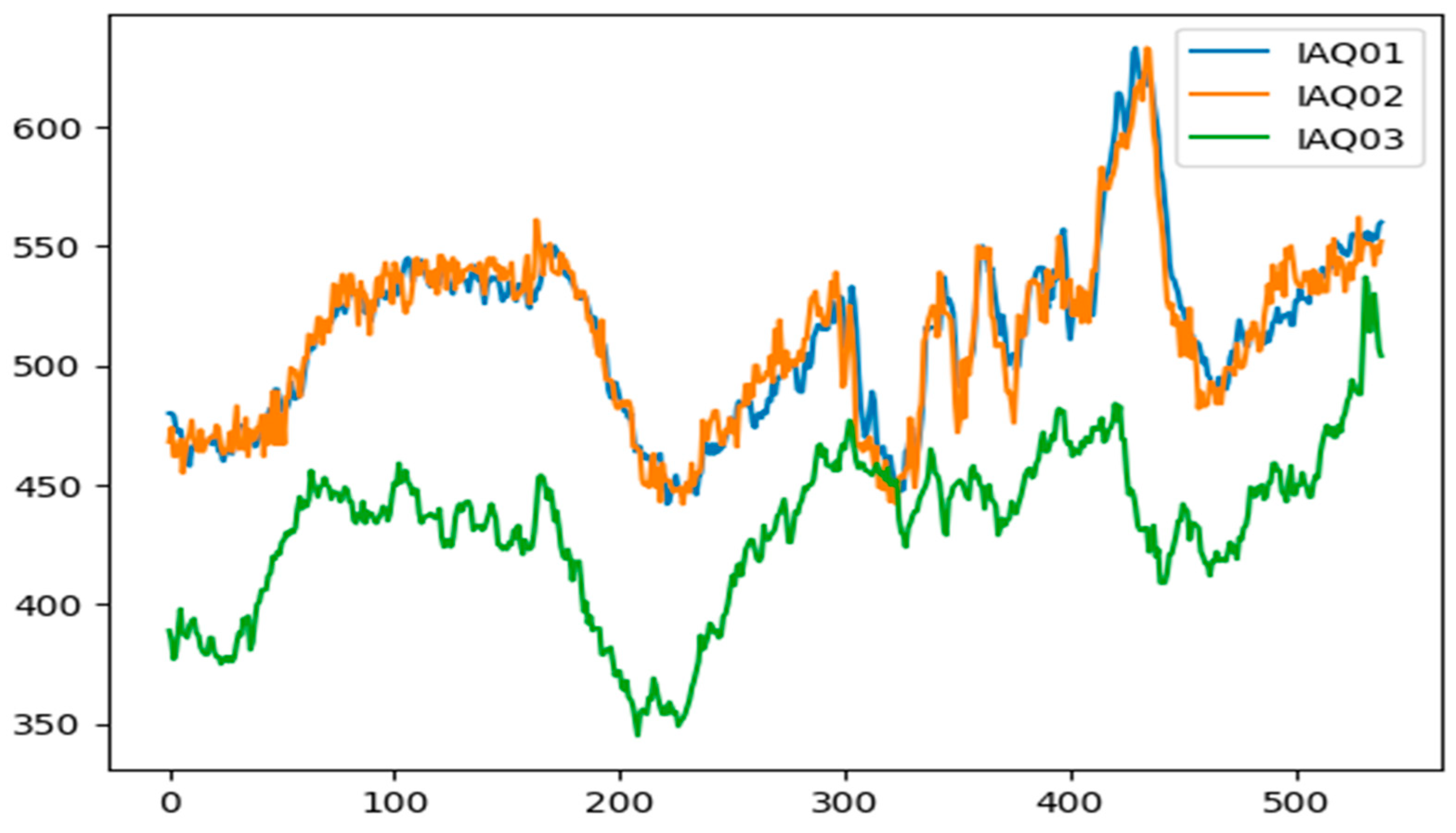
5.1. Experimental Results on an Office Dataset

For the evaluation, we set up 14 IAQ data points in an office space labeled from IAQ01 to IAQ14 as shown in Figure 2.
There is an IAQ sensor installed at each data point. In the figure, the lines represent the walls that segregate the rooms, the bottom left is defined as the origin, and the horizontal and the vertical arrows are the x- and the y-axes, respectively. Table 1 shows the specification of the CO2 and temperature sensors used in the office space.
Table 2 represents the coordinate values of the x-axis and y-axis of the 14 data points.
We developed a data collection system to collect the air quality data from the IAQ sensors. Figure 3 shows the architecture of the system.
Each sensor sends a packet, including the air quality data, every minute to the packet processing module of the system through the Transmission Control Protocol (TCP). The packet processing module parses the received packets and validates them. When the packets are valid, the data storing module stores them in the data repository. The stored data can be searched using the data searching module and displayed on the web in chart or table form.
In this experiment, we collected the CO2 concentration and temperature data every minute over a 5-day period from 29 June 2020 to 3 July 2020. For each of the 14 data points, we collected an average of 530 data points per day, totaling 37,086 data points for the CO2 concentration and temperature data, respectively. Using the June 29 data, we varied N from 2 to 7 and K between 3, 6, 9, 12, and 14 to find the N and K values with the minimum RMSE. Using the found N and K values, we performed interpolation experiments on the data from 30 June to 3 July to verify the performance.

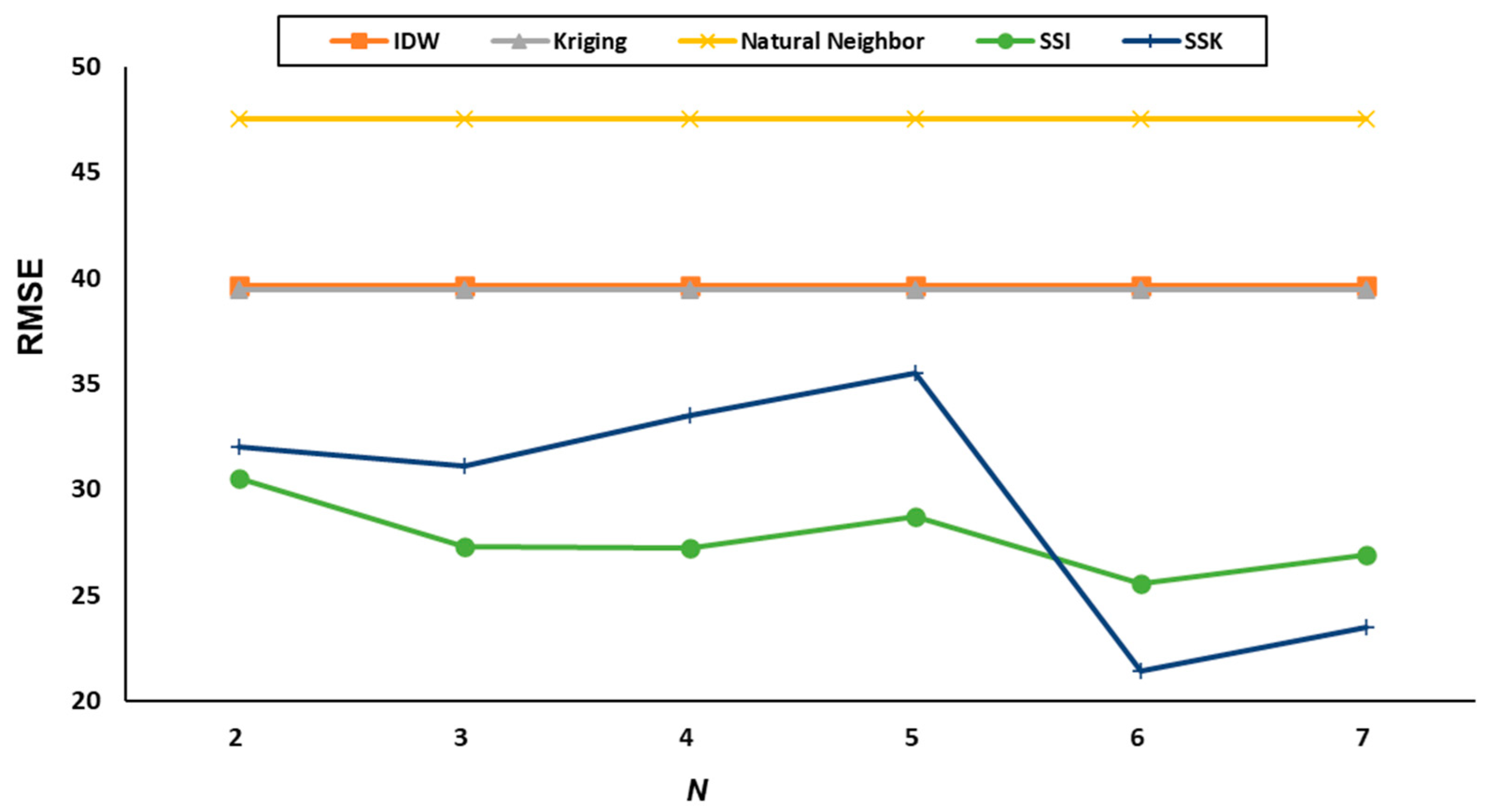
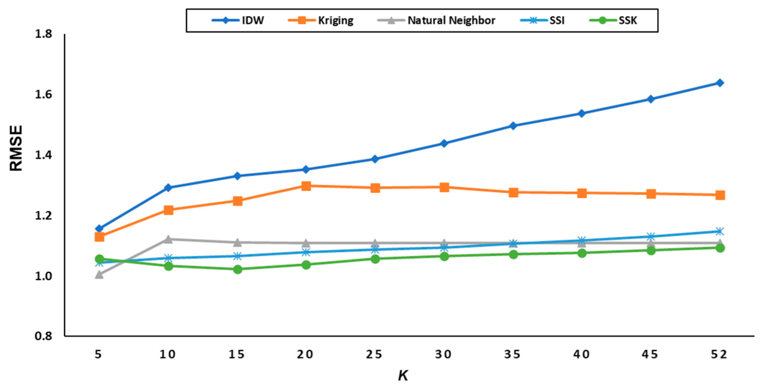
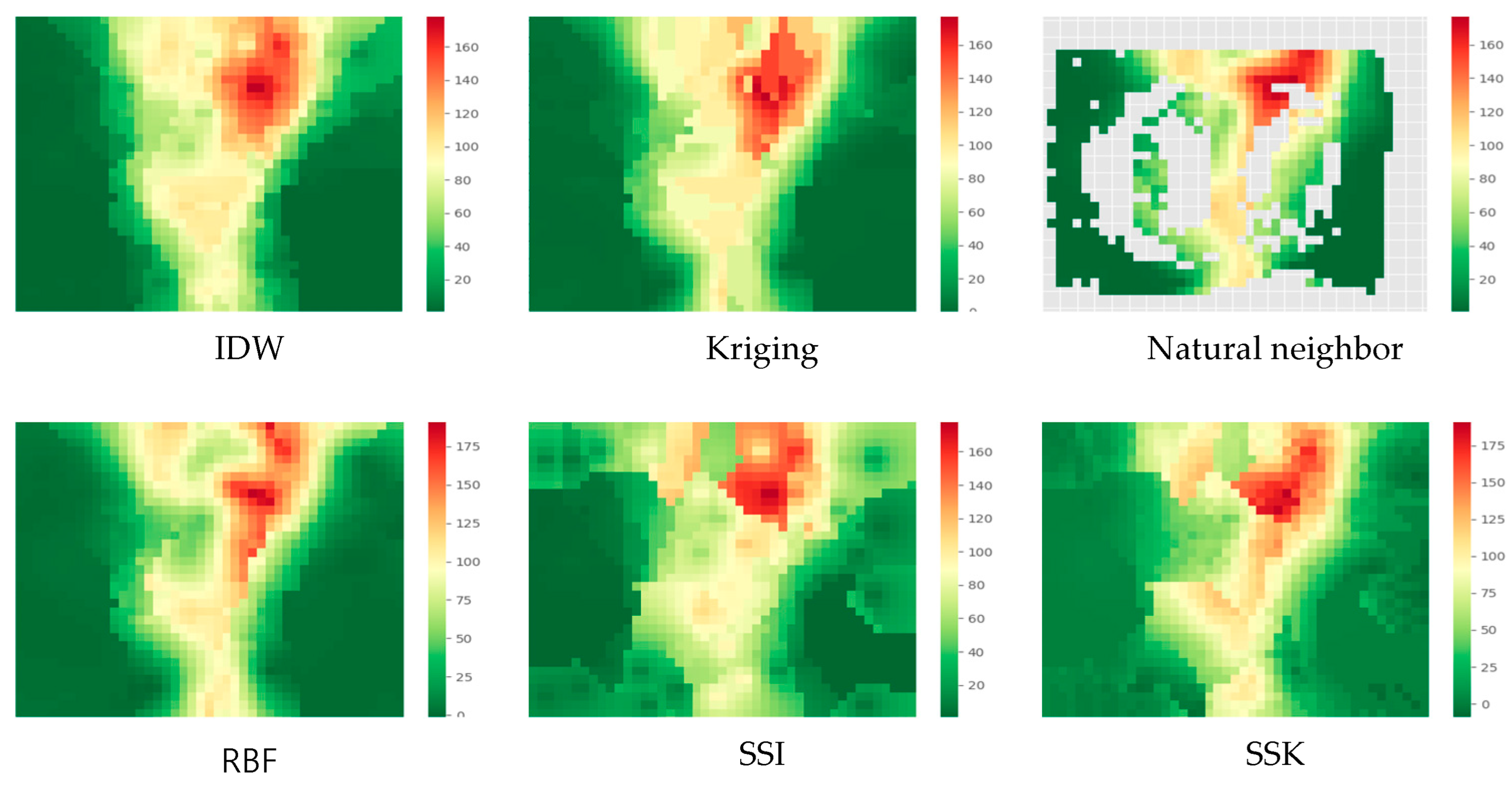
5.1.1. Experimental Results for CO2 Data

The color-coded representation of the groups assigned to each point in the office space through the group allocation and group assignment processes is shown in Figure 4. The number of groups varies from two to seven.
Table 3 presents the calculated RMSE values for each method as the number of groups N and the number of neighbors K for each N vary.
Figure 5 shows the RMSE values for each method when the number of groups in the CO2 data varies from two to seven. The RBF method is excluded from Figure 5 and the subsequent figures due to its large RMSE value compared to the other methods.
Figure 6 shows the RMSE values for each method when the number of neighbors varies from 3 to 14.
The IDW method had its minimum RMSE value when K = 14, the kriging method had its minimum RMSE value when K = 12, the natural neighbor method had its minimum RMSE value when K = 6, and the RBF method had its minimum RMSE value when K = 14. The SSI method had its minimum RMSE value when N = 6 and K = 3, and the SSK method had its minimum RMSE value when N = 6 and K = 6. Table 4 shows the results of a performance experiment using the optimal values of N and K for each method based on four days of data from 30 June to 3 July. As shown in Table 4, the proposed SSI and SSK methods show better performance metrics compared to the other methods.
Figure 7 shows the heatmaps for each method, displaying the estimated values for all the points when N = 5 and K = 6. In the case of the natural neighbor method, the areas outside the sensor range were not interpolated, so they are not displayed in the figure.

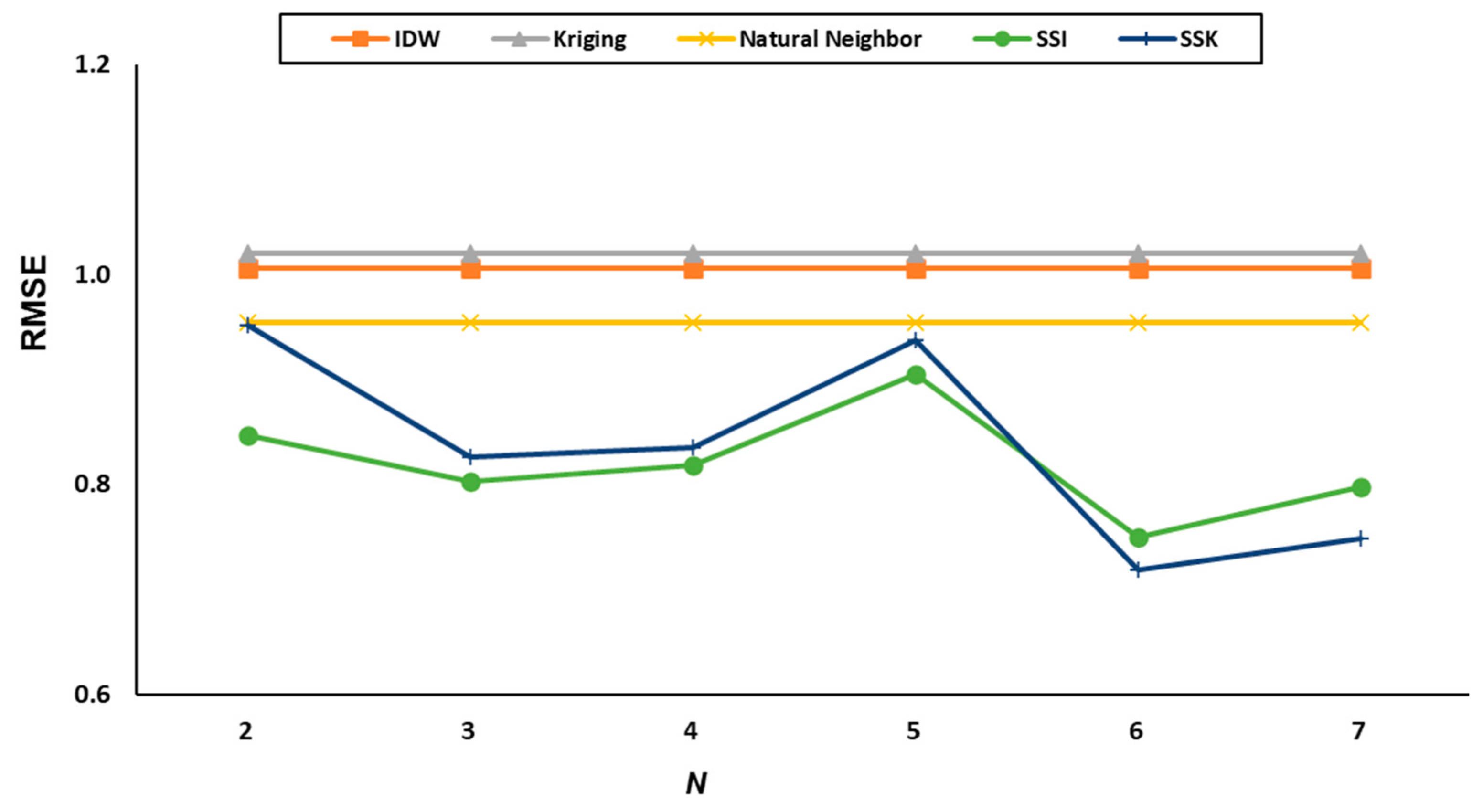
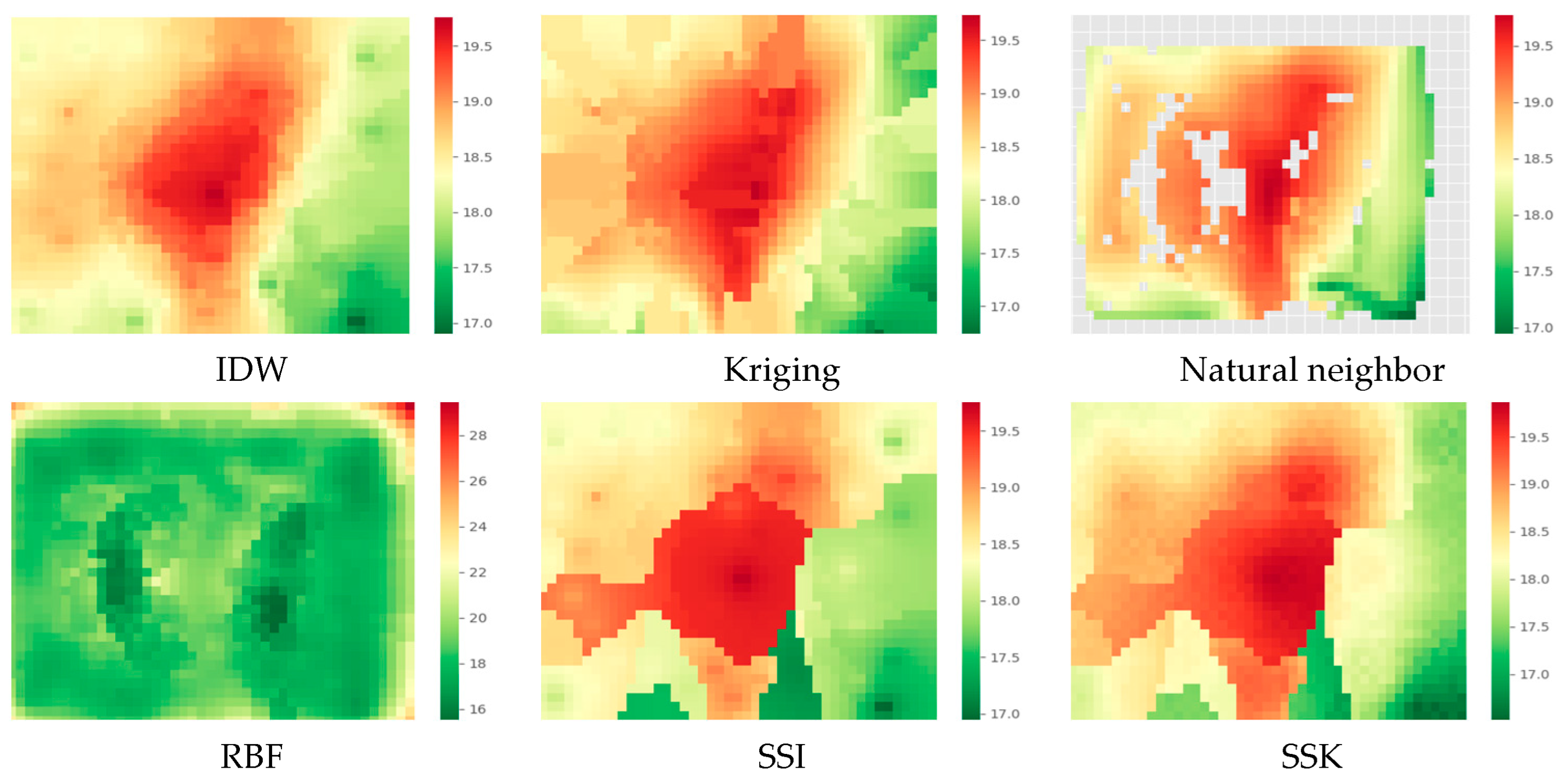
5.1.2. Experimental Results for Temperature Data

The color-coded representation of the groups assigned to each point in the office space through the group allocation and group assignment processes is shown in Figure 8. The number of groups varies from two to seven.
Table 5 presents the calculated RMSE values for each method as the number of groups N and the number of neighbors K for each N vary.
Figure 9 shows the RMSE values for each method as the number of groups in the temperature data varies from two to seven.
Figure 10 shows the RMSE values for each method when the number of neighbors in the temperature data varies from 3 to 14.
The IDW method had its minimum RMSE value when K = 3, the kriging method had its minimum RMSE value when K = 3, the natural neighbor method had its minimum RMSE value when K = 14, and the RBF method had its minimum RMSE value when K = 12. The SSI method had its minimum RMSE value when N = 6 and K = 6, and the SSK method had its minimum RMSE value when N = 6 and K = 12. Table 6 shows the results of a performance experiment using the optimal values of N and K for each method based on four days of data from 30 June to 3 July. As shown in Table 6, the proposed SSI and SSK methods show slightly better performance metrics compared to the other methods.
Figure 11 shows the heatmaps of the predicted values for each point when N = 5 and K = 6. For the natural neighbor method, the areas outside the sensor range were not interpolated and are not shown in the figure.
Figure 12 shows the CO2 values for IAQ01, IAQ02, and IAQ03 measured on 29 June.
From Figure 12, we can observe that the distance between IAQ02 and IAQ01 is greater than the distance between IAQ02 and IAQ03, but the data from IAQ02 and IAQ01 are much more similar than the data from IAQ02 and IAQ03. It is known that CO2 is highly correlated within an independent room separated by walls. Figure 13 shows the result of dividing the sensors into three groups based on the CO2 data using the group allocation and group assignment algorithms proposed in this paper. As shown in Figure 11, IAQ02 belongs to Group 1, the same group as IAQ01, while IAQ03 belongs to Group 3, a different group from IAQ01 and IAQ02.
Figure 14 shows the temperature values of IAQ03, IAQ10, and IAQ11 measured on 29 June.
From Figure 14, we can observe that the distance between IAQ11 and IAQ03 is greater than the distance between IAQ11 and IAQ10, but the data from IAQ11 and IAQ03 are much more similar than the data from IAQ11 and IAQ10. We think that this is likely due to the influence of various conditions, such as air conditioning and structure, in the office. Figure 15 shows the result of dividing the sensors into three groups based on the temperature data using the group allocation and group assignment algorithms proposed in this paper. As shown in Figure 11, IAQ11 belongs to Group 1, the same group as IAQ03, while IAQ10 belongs to Group3, a different group from IAQ11 and IAQ03.
Various IAQ parameters, including CO2, temperature, relative humidity, and light intensity, have distinct physics, and IAQ parameters are influenced not only by the layout of indoor spaces but also by these underlying physical properties. We assume that even if the physics of the IAQ parameters are different, the physics also would be reflected in the collected data. Therefore, we believe that the sensor grouping algorithm proposed in this paper partially reflects the spatial constraints on IAQ parameters.

5.2. Experimental Results Based on the Intel Lab Dataset

We evaluated our methods using the sensing data collected and made publicly available from Intel labs in 2004 [50,51]. This dataset provides the x and y coordinates of 54 sensors deployed in the Intel Berkeley Research lab between February 28th and April 5th, 2004. In the dataset, the temperature, humidity, light, and voltage data were collected at intervals of 31 s. The sensors were arranged in the lab according to Figure 16 [51].
For this experiment, we used five days of data from 28 February 2004 to 3 March 2004 averaged in minutes. Missing data were imputed using a linear method. Sensors 5 and 28 were excluded from the experiment due to a significant amount of missing data, resulting in a total of 52 sensors being used. We utilized the 28 February data for validation, meaning that we changed N to 3, 6, 9, 12, 15, 18, and 21 and K to 1, 10, 15, 20, 25, 30, 35, 40, 45, and 52 while utilizing the February 28 data to find the N and K values with the minimum RMSE. Using the found N and K values, we performed an interpolation experiment on the data from February 29 to March 3 to validate the performance.

5.2.1. Experimental Results for Temperature Data

Figure 17 shows the RMSE values for the experiment with the number of groups set to 3, 6, 9, 12, 15, 18, and 21 for the temperature data. The RBF method is excluded from the figure and the subsequent figures due to its large RMSE value compared to the other methods.
Figure 18 shows the RMSE values for the experiment with the number of neighbors set to 5, 10, 15, 20, 25, 30, 35, 40, 45, and 52 for the temperature data.
The IDW method had its minimum RMSE value when K = 5, the kriging method had its minimum RMSE value when K = 5, the natural neighbor method had its minimum RMSE value when K = 5, and the RBF method had its minimum RMSE value when K = 25. The SSI method had its minimum RMSE value when N = 6 and K = 5, and the SSK method had its minimum RMSE value when N = 6 and K = 30. Table 7 shows the results of performance experiments based on 4 days of data from February 29 to March 3 using the optimal values of N and K for each method. As shown in Table 7, the proposed SSI method provides slightly better performance metrics compared to the other methods, while the SSK method performs slightly worse in this case.
Figure 19 shows the heatmap of the predicted values for temperature.

5.2.2. Experimental Results for Humidity Data

Figure 20 shows the RMSE values for the experiment with the number of groups set to 3, 6, 9, 12, 15, 18, and 21 for the humidity data.
Figure 21 shows the RMSE values for the experiment with the number of neighbors set to 5, 10, 15, 20, 25, 30, 35, 40, 45, and 52 for the humidity data.
The IDW method had its minimum RMSE value when K = 5, the kriging method had its minimum RMSE value when K = 5, the natural neighbor method had its minimum RMSE value when K = 5, and the RBF method had its minimum RMSE value when K = 25. The SSI method had its minimum RMSE value when N = 6 and K = 5, and the SSK method had its minimum RMSE value when N = 9 and K = 15. Table 8 shows the results of performance experiments based on 4 days of data from 29 February to 3 March using the optimal values of N and K for each method. As shown in Table 8, the proposed SSI and SSK methods show slightly better performance metrics compared to the other methods.
Figure 22 shows the heatmap of the predicted values for humidity.

5.2.3. Experimental Results for Light Data

Figure 23 shows the RMSE values for the experiment with the number of groups set to 3, 6, 9, 12, 15, 18, and 21 for the light data.
Figure 24 shows the RMSE values for the experiment with the number of neighbors set to 5, 10, 15, 20, 25, 30, 35, 40, 45, and 52 for the light data.
The IDW method had its minimum RMSE value when K = 5, the kriging method had its minimum RMSE value when K = 5, the natural neighbor method had its minimum RMSE value when K = 5, and the RBF method had its minimum RMSE value when K = 25. The SSI method had its minimum RMSE value when N = 6 and K = 5, and the SSK method had its minimum RMSE value when N = 9 and K = 15. Table 9 shows the results of performance experiments based on 4 days of data from 29 February to 3 March using the optimal values of N and K for each method. As shown in Table 9, the proposed SSI and SSK methods show better performance metrics compared to the other methods.
Figure 25 shows the heatmap of the predicted values for light.

6. Conclusions

In this paper, we proposed an interpolation scheme for IAQ data that considers the spatial constraints of indoor environments. The proposed scheme was compared with commonly used methods, such as IDW, kriging, natural neighbor interpolation, and RBF, and was found to be more accurate in terms of the RMSE. The results of the experiment demonstrate that our proposed scheme could improve the accuracy of air quality estimation in indoor environments.
Our findings have important implications for IAQ management in various settings, including smart buildings, smart factories, schools, offices, and other similar environments. The accurate measurement and estimation of air quality parameters are crucial for maintaining occupant health and comfort and optimizing energy use in indoor spaces. Our proposed interpolation scheme can provide more accurate estimates of air quality parameters, which can inform the optimization of ventilation and air conditioning systems and ultimately lead to a healthier indoor environment for occupants. The integration of IAQ estimation with energy management and occupant behavior modeling can lead to more comprehensive and effective IAQ management strategies. In this paper, a DCP-based k-mode clustering method is used to group sensors with similar characteristics. However, the performance of the proposed spatial interpolation method may be affected when the internal structure of the indoor space is changed. To address this, further research is needed on how to regroup sensors when the performance is degraded or the indoor space is changed. Additionally, this study does not include an analysis of important factors related to indoor air quality, such as particulate matter (PM) and volatile organic compounds (VOCs), which presents an area for future research.

Author Contributions

Conceptualization, Seungwoog Jung; investigation, Seungwoog Jung and Seungwan Han; methodology, Seungwoog Jung and Hoon Choi; software and validation, Seungwoog Jung and Seungwan Han, writing—original draft, Seungwoog Jung; writing—review and editing, Seungwan Han and Hoon Choi. All authors have read and agreed to the published version of the manuscript.

Funding

This research was supported by research fund of Chungnam National University (2021-0862-01).

Data Availability Statement

The Intel Lab data are available at http://db.csail.mit.edu/labdata/labdata.html (accessed on 10 May 2023). The office data presented in this study are available from the authors based on a reasonable request.

Acknowledgments

The authors thank the managing editor and anonymous reviewers for their constructive comments.

Conflicts of Interest

The authors declare no conflict of interest.

References

  1. Kim, H.; Hong, T.; Kim, J.; Yeom, S. A psychophysiological effect of indoor thermal condition on college students’ learning performance through EEG measurement. Build. Environ. 2020, 184, 107223. [Google Scholar] [CrossRef]
  2. Andargie, M.S.; Azar, E. An applied framework to evaluate the impact of indoor office environmental factors on occupants’ comfort and working conditions. Sustain. Cities Soc. 2019, 46, 101447. [Google Scholar] [CrossRef]
  3. Frontczak, M.; Wargocki, P. Literature survey on how different factors influence human comfort in indoor environments. Build. Environ. 2011, 46, 922–937. [Google Scholar] [CrossRef]
  4. Calvo, I.; Espin, A.; Gil-García, J.M.; Fernández Bustamante, P.; Barambones, O.; Apiñaniz, E. Scalable IoT Architecture for Monitoring IEQ Conditions in Public and Private Buildings. Energies 2022, 15, 2270. [Google Scholar] [CrossRef]
  5. Dong, B.; Prakash, V.; Feng, F.; O’Neill, Z. A review of smart building sensing system for better indoor environment control. Energy Build. 2019, 199, 29–46. [Google Scholar] [CrossRef]
  6. Afonso, J.A.; Monteiro, V.; Afonso, J.L. Internet of things systems and applications for smart buildings. Energies 2023, 16, 2757. [Google Scholar] [CrossRef]
  7. Ma, C.; Guerra-Santin, O.; Grave, A.; Mohammadi, M. Supporting dementia care by monitoring indoor environmental quality in a nursing home. Indoor Built Environ. 2023. [Google Scholar] [CrossRef]
  8. Albu, A.V.; Caciora, T.; Berdenov, Z.; Ilies, D.C.; Sturzu, B.; Sopota, D.; Herman, G.V.; Ilies, A.; Kecse, G.; Ghergheles, C.G. Digitalization of garment in the context of circular economy. Ind. Text. 2021, 72, 102–107. [Google Scholar] [CrossRef]
  9. Bourdeau, M.; Waeytens, J.; Aouani, N.; Basset, P.; Nefzaoui, E. A Wireless Sensor Network for Residential Building Energy and Indoor Environmental Quality Monitoring: Design, Instrumentation, Data Analysis and Feedback. Sensors 2023, 23, 5580. [Google Scholar] [CrossRef]
  10. Boumpoulis, V.; Michalopoulou, M.; Depountis, N. Comparison between different spatial interpolation methods for the development of sediment distribution maps in coastal areas. Earth Sci. Inform. 2023, 1–19. [Google Scholar] [CrossRef]
  11. Zhu, D.; Cheng, X.; Zhang, F.; Yao, X.; Gao, Y.; Liu, Y. Spatial interpolation using conditional generative adversarial neural networks. Int. J. Geogr. Inf. Sci. 2020, 34, 735–758. [Google Scholar] [CrossRef]
  12. Comber, A.; Zeng, W. Spatial interpolation using areal features: A review of methods and opportunities using new forms of data with coded illustrations. Geogr. Compass 2019, 13, e12465. [Google Scholar] [CrossRef]
  13. Martínez-Comesaña, M.; Ogando-Martínez, A.; Troncoso-Pastoriza, F.; López-Gómez, J.; Febrero-Garrido, L.; Granada-Álvarez, E. Use of optimised MLP neural networks for spatiotemporal estimation of indoor environmental conditions of existing buildings. Build. Environ. 2021, 205, 108243. [Google Scholar] [CrossRef]
  14. Choi, H.; Kim, H.; Yeom, S.; Hong, T.; Jeong, K.; Lee, J. An indoor environmental quality distribution map based on spatial interpolation methods. Build. Environ. 2022, 213, 108880. [Google Scholar] [CrossRef]
  15. Jin, M.; Liu, S.; Schiavon, S.; Spanos, C. Automated mobile sensing: Towards high-granularity agile indoor environmental quality monitoring. Build. Environ. 2018, 127, 268–276. [Google Scholar] [CrossRef]
  16. Cheng, J.C.; Kwok, H.H.; Li, A.T.; Tong, J.C.; Lau, A.K. BIM-supported sensor placement optimization based on genetic algorithm for multi-zone thermal comfort and IAQ monitoring. Build. Environ. 2022, 216, 108997. [Google Scholar] [CrossRef]
  17. Choi, K.; Chong, K. Modified inverse distance weighting interpolation for particulate matter estimation and mapping. Atmosphere 2022, 13, 846. [Google Scholar] [CrossRef]
  18. Kaligambe, A.; Fujita, G.; Keisuke, T. Estimation of Unmeasured Room Temperature, Relative Humidity, and CO2 Concentrations for a Smart Building Using Machine Learning and Exploratory Data Analysis. Energies 2022, 15, 4213. [Google Scholar] [CrossRef]
  19. Zhou, X.; Guo, Q.; Han, J.; Wang, J.; Lu, Y.; Shi, J.; Kou, M. Real-time prediction of indoor humidity with limited sensors using cross-sample learning. Build. Environ. 2022, 215, 108964. [Google Scholar] [CrossRef]
  20. Ma, J.; Ding, Y.; Cheng, J.C.; Jiang, F.; Wan, Z. A temporal-spatial interpolation and extrapolation method based on geographic Long Short-Term Memory neural network for PM2. 5. J. Clean. Prod. 2019, 237, 117729. [Google Scholar] [CrossRef]
  21. Huang, Y.; Shen, X.; Li, J.; Li, B.; Duan, R.; Lin, C.H.; Chen, Q. A method to optimize sampling locations for measuring indoor air distributions. Atmos. Environ. 2015, 102, 355–365. [Google Scholar] [CrossRef]
  22. Collins, F.C. A Comparison of Spatial Interpolation Techniques in Temperature Estimation. Ph.D. Thesis, Virginia Tech, Blacksburg, VA, USA, November 1995. [Google Scholar]
  23. Dhamodaran, S.; Lakshmi, M. Comparative analysis of spatial interpolation with climatic changes using inverse distance method. J. Ambient. Intell. Humaniz. Comput. 2021, 12, 6725–6734. [Google Scholar] [CrossRef]
  24. Wang, D.W.; Li, L.N.; Hu, C.; Li, Q.; Chen, X.; Huang, P.W. A modified inverse distance weighting method for interpolation in open public places based on Wi-Fi probe data. J. Adv. Transp. 2019. [Google Scholar] [CrossRef]
  25. Yudison, A.P. Development of Indoor Air Pollution Concentration Prediction by Geospatial Analysis. J. Eng. Technol. Sci. 2015, 47, 306–319. [Google Scholar]
  26. Li, Z.; Wang, K.; Ma, H.; Wu, Y. An adjusted inverse distance weighted spatial interpolation method. In Proceedings of the 2018 3rd International Conference on Communications, Information Management and Network Security (CIMNS 2018), Wuhan, China, 27 September 2018; Advances in Computer Science Research; Atlantis Press: Amsterdam, The Netherlands, 2018. [Google Scholar]
  27. Smith, T.E. Spatial Interpolation Models. In Notebook on Spatial Data Analysis; University of Pennsylvania: Philadelphia, PA, USA, 2014; Available online: https://www.seas.upenn.edu/~tesmith/NOTEBOOK/index.html (accessed on 15 March 2021).
  28. Di Salvo, F.; Ruggieri, M.; Plaia, A. Extending Functional kriging to a multivariate context. Int. J. Stat. Anal. 2020, 18, 1–20. [Google Scholar]
  29. Ignaccolo, R.; Mateu, J.; Giraldo, R. Kriging with external drift for functional data for air quality monitoring. Stoch. Environ. Res. Risk Assess. 2014, 28, 1171–1186. [Google Scholar] [CrossRef]
  30. Adhikary, S.K.; Muttil, N.; Yilmaz, A.G. Genetic programming-based ordinary kriging for spatial interpolation of rainfall. J. Hydrol. Eng. 2016, 21, 04015062. [Google Scholar] [CrossRef]
  31. Zhang, J.; Li, X.; Yang, R.; Liu, Q.; Zhao, L.; Dou, B. An extended kriging method to interpolate near-surface soil moisture data measured by wireless sensor networks. Sensors 2017, 17, 1390. [Google Scholar] [CrossRef]
  32. Jha, D.K.; Sabesan, M.; Das, A.; Vinithkumar, N.V.; Kirubagaran, R. Evaluation of Interpolation Technique for Air Quality Parameters in Port Blair, India. Univers. J. Environ. Res. Technol. 2011, 1, 301–310. [Google Scholar]
  33. Oktavia, E.; Mustika, I.W. Inverse distance weighting and kriging spatial interpolation for data center thermal monitoring. In Proceedings of the 2016 1st International Conference on Information Technology, Information Systems and Electrical Engineering (ICITISEE), Yogyakarta, Indonesia, 23–24 August 2016; pp. 69–74. [Google Scholar]
  34. Sibson, R. A brief description of natural neighbour interpolation. In Interpreting Multivariate Data; Barnett, V., Ed.; John Wiley & Sons: New York, NY, USA, 1981; pp. 21–36. [Google Scholar]
  35. Bobach, T.A. Natural Neighbor Interpolation-Critical Assessment and New Contributions. Ph.D. Thesis, Technische Universität Kaiserslautern, Kaiserslautern, Germany, April 2008. [Google Scholar]
  36. Musashi, J.P.; Pramoedyo, H.; Fitriani, R. Comparison of inverse distance weighted and natural neighbor interpolation method at air temperature data in Malang region. CAUCHY J. Mat. Murni Dan Apl. 2018, 5, 48–54. [Google Scholar] [CrossRef]
  37. Schulte, N.; Li, X.; Ghosh, J.K.; Fine, P.M.; Epstein, S.A. Responsive high-resolution air quality index mapping using model, regulatory monitor, and sensor data in real-time. Environ. Res. Lett. 2020, 15, 1040a7. [Google Scholar] [CrossRef]
  38. Etherington, T.R. Discrete natural neighbour interpolation with uncertainty using cross-validation error-distance fields. PeerJ Comput. Sci. 2020, 6, e282. [Google Scholar] [CrossRef] [PubMed]
  39. Bobach, T.; Umlauf, G. Natural Neighbor Interpolation and Order of Continuity. In Proceedings of the First Workshop of the DFG’s International Research Training Group “Visualization of Large and Unstructured Data Sets—Applications in Geospatial Planning, Modeling, and Engineering”, Dagstuhl, Germany, 14–16 June 2006; Hagen, H., Kerren, A., Dannenmann, P., Eds.; Gesellschaft für Informatik (GI): Bonn, Germany, 2006. [Google Scholar]
  40. Beutel, A.; Mølhave, T.; Agarwal, P.K. Natural neighbor interpolation based grid DEM construction using a GPU. In Proceedings of the 18th SIGSPATIAL International Conference on Advances in Geographic Information Systems, San Jose, CA, USA, 2–5 November 2010; Association for Computing Machinery: New York, NY, USA, 2010; pp. 172–181. [Google Scholar]
  41. Zou, B.; Wang, M.; Wan, N.; Wilson, J.G.; Fang, X.; Tang, Y. Spatial modeling of PM 2.5 concentrations with a multifactoral radial basis function neural network. Environ. Sci. Pollut. Res. 2015, 22, 10395–10404. [Google Scholar] [CrossRef] [PubMed]
  42. Losser, T.; Li, L.; Piltner, R. A spatiotemporal interpolation method using radial basis functions for geospatiotemporal big data. In Proceedings of the 2014 Fifth International Conference on Computing for Geospatial Research and Application, Washington, DC, USA, 4–6 August 2014. [Google Scholar]
  43. Sajjadi, S.A.; Zolfaghari, G.; Adab, H.; Allahabadi, A.; Delsouz, M. Measurement and modeling of particulate matter concentrations: Applying spatial analysis and regression techniques to assess air quality. MethodsX 2017, 4, 372–390. [Google Scholar] [CrossRef] [PubMed]
  44. Ha, Q.P.; Wahid, H.; Duc, H.; Azzi, M. Enhanced radial basis function neural networks for ozone level estimation. Neurocomputing 2015, 155, 62–70. [Google Scholar] [CrossRef]
  45. Chen, C.S.; Noorizadegan, A.; Young, D.L.; Chen, C.S. On the selection of a better radial basis function and its shape parameter in interpolation problems. Appl. Math. Comput. 2023, 442, 127713. [Google Scholar] [CrossRef]
  46. Huang, Z. Extensions to the k-means algorithm for clustering large data sets with categorical values. Data Min. Knowl. Discov. 1998, 2, 283–304. [Google Scholar] [CrossRef]
  47. Selim, S.Z.; Ismail, M.A. K-means-type algorithms: A generalized convergence theorem and characterization of local optimality. IEEE Trans. Pattern Anal. Mach. Intell. 1984, 6, 81–87. [Google Scholar] [CrossRef]
  48. San, O.M.; Huynh, V.N.; Nakamori, Y. An alternative extension of the k-means algorithm for clustering categorical data. Int. J. Appl. Math. Comput. Sci. 2004, 14, 241–247. [Google Scholar]
  49. Chicco, D.; Warrens, M.J.; Jurman, G. The coefficient of determination R-squared is more informative than SMAPE, MAE, MAPE, MSE and RMSE in regression analysis evaluation. PeerJ Comput. Sci. 2021, 7, e623. [Google Scholar] [CrossRef]
  50. Heo, T.; Kim, H.; Ko, J.; Doh, Y.; Park, J.; Jun, J.; Choi, H. Adaptive dual prediction scheme based on sensing context similarity for wireless sensor networks. Electron. Lett. 2014, 50, 467–469. [Google Scholar] [CrossRef]
  51. Intel Lab Data. Available online: http://db.csail.mit.edu/labdata/labdata.html (accessed on 3 July 2021).
Figure 1. Flowchart of the proposed spatial interpolation scheme.
Ijgi 12 00347 g001
Figure 2. Experimental testbed composed of 14 air quality data points labeled from IAQ01 to IAQ14.
Ijgi 12 00347 g002
Figure 3. Data collection system used to collect air quality data from IAQ sensors.
Ijgi 12 00347 g003
Figure 4. Color-coded representation of groups for CO2, with the number of groups being 2 to 7.
Ijgi 12 00347 g004
Figure 5. RMSE plot by number of groups for CO2 data.
Ijgi 12 00347 g005
Figure 6. RMSE plot by the number of neighbors for CO2 data.
Ijgi 12 00347 g006
Figure 7. Heatmap plots for CO2 data when N = 5 and K = 6.
Ijgi 12 00347 g007
Figure 8. Color-coded representation of groups for temperature, with the number of groups being 2 to 7.
Ijgi 12 00347 g008
Figure 9. RMSE plot by number of groups for temperature data.
Ijgi 12 00347 g009
Figure 10. RMSE plot by number of neighbors for temperature data.
Ijgi 12 00347 g010
Figure 11. Heatmap plots for temperature data when N = 5 and K = 6.
Ijgi 12 00347 g011
Figure 12. Graph comparing CO2 data for IAQ01, IAQ02, and IAQ03.
Ijgi 12 00347 g012
Figure 13. Color-coded representation of groups for CO2 with a group number of 3. Group 1 includes IAQ01, IAQ02, IAQ06, IAQ07, and IAQ09; Group 2 includes IAQ04, IAQ05, IAQ11, IAQ13, and IAQ14; and Group 3 includes IAQ03, IAQ10, IAQ08, and IAQ12.
Ijgi 12 00347 g013
Figure 14. Graph comparing temperature data for IAQ03, IAQ10, and IAQ11.
Ijgi 12 00347 g014
Figure 15. Color-coded representation of groups for temperature with a group number of 3. Group 1 includes IAQ01, IAQ02, IAQ03, IAQ04, IAQ11, IAQ12, IAQ13, and IAQ14; Group 2 includes IAQ05 and IAQ06; and Group 3 includes IAQ07, IAQ08, IAQ09, and IAQ10.
Ijgi 12 00347 g015
Figure 16. Arrangement of sensors in Intel Lab. The numbers 1 through 54 indicate where each sensor is installed.
Ijgi 12 00347 g016
Figure 17. RMSE plot for Intel Lab temperature data by number of groups.
Ijgi 12 00347 g017
Figure 18. RMSE plot for Intel Lab temperature data by number of neighbors.
Ijgi 12 00347 g018
Figure 19. Heatmap plots for temperature data when N = 5 and K = 7.
Ijgi 12 00347 g019
Figure 20. RMSE plot for Intel Lab humidity data by number of groups.
Ijgi 12 00347 g020
Figure 21. RMSE plot for Intel Lab humidity data by number of neighbors.
Ijgi 12 00347 g021
Figure 22. Heatmap plots for humidity data when N = 5 and K = 7.
Ijgi 12 00347 g022
Figure 23. RMSE plot for Intel Lab light data by number of groups.
Ijgi 12 00347 g023
Figure 24. RMSE plot for Intel Lab temperature data by number of neighbors.
Ijgi 12 00347 g024
Figure 25. Heatmap plots for light data when N = 5 and K = 7.
Ijgi 12 00347 g025
Table 1. Specification of CO2 and temperature sensors used in the office space.
SensorCO2Temperature
ModelE + ESensirion
Range0~2000 ppm−4~125 °C
Accuracy<±50 ppm + 2%±0.3 °C ± 2%
InterfaceI2CI2C
Country of manufactureAustriaSwitzerland
Table 2. Coordinate values of each data point.
Data PointX Location (cm)Y Location (cm)
IAQ01100243
IAQ02126354
IAQ03187335
IAQ04265249
IAQ05392335
IAQ06511283
IAQ07637384
IAQ08387178
IAQ09507111
IAQ10603176
IAQ113258
IAQ1238615
IAQ1359119
IAQ1462354
Table 3. RMSE values by the number of groups and number of neighbors for CO2 data.
NKIDWKrigingNatural NeighborRBFSSISSK
23 43.2641.4259.62241.9431.0429.96
6 39.8038.5041.66177.3829.7130.47
9 38.9339.9141.86159.0830.0732.06
12 38.1138.3647.18156.9430.6932.83
14 38.0039.1047.18155.2031.0534.74
33 43.2641.4259.62241.9425.7926.54
6 39.8038.5041.66177.3826.3727.22
9 38.9339.9141.86159.0826.9729.65
12 38.1138.3647.18156.9428.5633.79
14 38.0039.1047.18155.2028.8738.17
43 43.2641.4259.62241.9426.0324.00
6 39.8038.5041.66177.3826.5426.12
9 38.9339.9141.86159.0826.8033.52
12 38.1138.3647.18156.9428.3040.42
14 38.0039.1047.18155.2028.6043.37
53 43.2641.4259.62241.9426.5924.36
6 39.8038.5041.66177.3828.3228.94
9 38.9339.9141.86159.0829.1234.86
12 38.1138.3647.18156.9429.5642.54
14 38.0039.1047.18155.2029.9346.72
63 43.2641.4259.62241.9422.8222.51
6 39.8038.5041.66177.3823.9720.90
9 38.9339.9141.86159.0825.8521.13
12 38.1138.3647.18156.9427.0921.11
14 38.0039.1047.18155.2027.9121.43
73 43.2641.4259.62241.9425.7925.54
6 39.8038.5041.66177.3825.4423.41
9 38.9339.9141.86159.0826.8622.86
12 38.1138.3647.18156.9427.7122.52
14 38.0039.1047.18155.2028.5522.96
Table 4. Performance metrics for each method implemented with optimal N and K for CO2 data collected from 30 June to 3 July.
MethodIDWKrigingNatural NeighborRBFSSISSK
RMSE45.4446.0443.98175.4228.8426.66
MAE38.8437.9638.78166.4323.3521.71
MAPE10.219.9410.9739.1210.138.00
R20.400.420.340.070.510.57
Table 5. RMSE values by the number of groups and the number of neighbors for temperature data.
NKIDWKrigingNatural NeighborRBFSSISSK
23 0.980.990.9612.860.880.94
6 0.991.020.9510.210.830.88
9 0.991.030.968.150.830.99
12 1.021.030.957.900.850.95
14 1.051.020.958.090.851.00
33 0.980.990.9612.860.780.86
6 0.991.020.9510.210.750.81
9 0.991.030.968.150.770.83
12 1.021.030.957.900.840.81
14 1.051.020.958.090.870.83
43 0.980.990.9612.860.810.88
6 0.991.020.9510.210.770.81
9 0.991.030.968.150.780.84
12 1.021.030.957.900.850.82
14 1.051.020.958.090.890.83
53 0.980.990.9612.860.910.99
6 0.991.020.9510.210.830.90
9 0.991.030.968.150.850.97
12 1.021.030.957.900.940.90
14 1.051.020.958.090.980.92
63 0.980.990.9612.860.690.73
6 0.991.020.9510.210.660.72
9 0.991.030.968.150.720.72
12 1.021.030.957.900.810.71
14 1.051.020.958.090.860.72
73 0.980.990.9612.860.710.74
6 0.991.020.9510.210.710.71
9 0.991.030.968.150.760.76
12 1.021.030.957.900.880.76
14 1.051.020.958.090.940.78
Table 6. Performance metrics for each method implemented with optimal N and K for temperature data collected from 30 June to 3 July.
MethodIDWKrigingNatural NeighborRBFSSISSK
RMSE1.071.091.067.640.810.88
MAE0.910.900.937.250.660.72
MAPE4.664.784.1335.254.024.37
R20.360.350.360.020.430.41
Table 7. Performance metrics values for each method implemented with optimal N and K for Intel Lab temperature data collected from 29 February to 3 March.
MethodIDWKrigingNatural NeighborRBFSSISSK
RMSE2.382.452.445.901.862.90
MAE1.922.132.114.661.782.43
MAPE10.1912.2010.7735.099.0114.93
R20.720.670.740.190.770.73
Table 8. Performance metrics for each method implemented with optimal N and K for Intel Lab humidity data collected from 29 February to 3 March.
MethodIDWKrigingNatural NeighborRBFSSISSK
RMSE1.851.851.777.571.551.60
MAE1.521.391.435.571.231.26
MAPE6.216.134.7212.834.194.25
R20.860.880.890.320.930.93
Table 9. Performance metrics for each method implemented with optimal N and K for Intel Lab light data collected from 29 February to 3 March.
MethodIDWKrigingNatural NeighborRBFSSISSK
RMSE170.22161.47139.71175.8884.4690.47
MAE137.10122.95112.15132.3264.7268.41
MAPE17.0815.7514.6518.248.649.35
R20.490.500.690.440.750.72
Disclaimer/Publisher’s Note: The statements, opinions and data contained in all publications are solely those of the individual author(s) and contributor(s) and not of MDPI and/or the editor(s). MDPI and/or the editor(s) disclaim responsibility for any injury to people or property resulting from any ideas, methods, instructions or products referred to in the content.

