Urban Resident Travel Survey Method Based on Cellular Signaling Data

Abstract

A low-cost, timely, and durable long-term approach to resident travel surveys is crucial for authorities to understand the city’s transportation systems and formulate transportation planning and management policies. This paper summarizes commonly used wireless positioning technologies and uses the STDBSCAN method to identify travel endpoints based on the characteristics of trajectory location information. It uses Shenzhen cellular signaling data to visually analyze the spatial and temporal distribution of urban traffic demand, traffic correlation, and asymmetry of traffic flow between different traffic zones. The results confirm that mobile internet information represented by cellular signaling information can effectively reflect the traffic status of urban areas, which, compared to traditional travel survey methods, has the advantages of lower cost, more timely feedback, and can be durably carried out in the long term.

1. Introduction

The transportation system is an indispensable component of the regular operation of cities, significantly impacting the construction of urban industry and the daily lives of urban residents. A good transportation system can improve travel efficiency, promote urban economic development, and improve residents’ quality of life [1,2].

Transportation planning guides the construction of the whole urban traffic system. Good transportation planning can ensure that the number of traffic facilities in the entire city is appropriate and that the layout is reasonable and promote coordination between different traffic departments. It includes road planning, public transportation planning, parking lot planning, non-motorized transportation planning, etc. It involves all aspects of the transportation system, plays a vital role in the construction of the transportation system, and is the construction program of the entire urban transportation system [3,4].

Transportation planning needs to comprehensively consider the city’s economic, social, environmental, and other factors. The resident travel survey is an essential reference for transportation planning. The resident travel survey mainly uses household interview surveys, and to master the comprehensive travel characteristics of urban residents, the interview will involve multiple aspects such as family (income, address, number of family members, held-vehicle of house-hold), individual (occupation, age, gender), and single travel (origin, destination, purpose, duration time, distance, travel mode) characteristics. Through analysis of the resident travel survey, the traffic management department can formulate more scientific and reasonable transportation planning and management schemes according to the actual travel situation of urban residents and the needs of urban development [5,6]. For example, by comparing the capacity of present roads with the travel needs of residents, the resident travel survey can guide the construction of future roads and the improvement of existing roads. Based on the changing travel needs of residents over time, authorities can draw up targeted routine and peak-hour management plans [7]. Based on the survey results on the travel purposes and needs of residents, bus companies can draw up better vehicle scheduling plans and bus routes to better meet the travel needs of residents and increase load factors [8]. The resident travel survey has a guiding significance for urban transportation system planning, design, and management. The construction of various aspects, such as public transportation, non-motorized transportation, and static transportation, requires resident travel data as support.

The resident travel survey needs to analyze the entire travel process from start to end, which involves a comprehensive investigation of travel generation, mode of travel, purpose of travel, travel time, etc. In addition to surveying the travel itself, the resident travel survey also includes statistics on the attributes of the travelers carrying out the travel and the attributes of the traveler’s family. The resident travel survey is costly due to its multifarious survey items and the fact that most of resident travel surveys are in the form of home visits, which require the involvement of a large number of people in the survey process [9]. On the other hand, with the construction and development of cities, the travel rules of residents will ceaselessly change, leading to the timeliness of the results of the resident travel survey [10]. To grasp the latest travel rules in time, it is necessary to organize the resident travel survey continuously and regularly.

The earliest resident travel surveys were carried out to better plan road construction to meet traffic demand. On 20 December 1944, the United States Congress passed the Federal-Aid Highways Act of 1944. This act provided USD 1.5 billion in spending for 6400 km of the National System of Interstate Highways to connect major cities and industrial areas. Due to the lack of sufficient travel information on residents in road planning and construction, the Public Roads Administration (PRA) proposed the method of home-interview origin–destination surveys. The PRA compiled the survey procedure manual based on the needs of the survey, and it has been gradually applied in many countries and cities as a general mode of transportation survey.

Today, the National Household Travel Survey (NHTS), conducted by the Federal Highway, is a long-running and widespread survey [11]. The NHTS is the source of the nation’s information about travel by US residents in all 50 States and the District of Columbia. Federal and state agencies use the survey results to monitor the performance and adequacy of current facilities and infrastructure and to plan for future needs. State and regional agencies use the data to support travel demand modeling and long-range transportation planning. Data from the NHTS are included in broader, bi-annual reports to Congress on the performance of the surface transportation system. Survey data are also applied outside of transportation in the fields of public health, environmental analysis, energy consumption, and social welfare. In the NHTS Data User Guide, some common data usage scenarios are mentioned as examples, such as describing and analyzing current travel, developing trends of transportation systems over time, energy consumption, environmental concerns, and modeling and planning applications [12].

Britain’s first National Travel Survey (NTS) was carried out by the Ministry of Transport in 1965. In July 1988, the NTS became a continuous survey with an annual sample size of 5040 addresses. The annual sample increased to 5796 addresses by 2001 and 15,048 addresses by 2002. Since January 2002, the Department for Transport (DfT) has commissioned the National Centre for Social Research (NatCen), an independent social research institute, as the contractor for the NTS. NatCen is responsible for questionnaire development, sample selection, data collection and editing, data file production, and database building. The DfT is responsible for data analysis, publication, and archiving.

The NTS collects detailed information on the critical characteristics of each participating household and any vehicle to which they have access. In addition, everyone within the household is interviewed and asked to complete a seven-day travel diary [13]. Data from the NTS are used extensively by the DfT to monitor changes in travel patterns and to inform the development of policy [14,15,16]. The findings and data are also used by a variety of other organizations, including other government departments (such as HM Revenue and Customs, HM Treasury, the Department for Environment, Food and Rural Affairs), university academics and students, transport consultants, local authorities, and voluntary sector organizations [17,18,19].

Resident travel surveys are collected using various means, including home visits, telephone surveys, mail surveys, etc., with home visits being the most extensive. Home visit surveys require investigators to survey selected households following under-sampling rules. With the cooperation of the respondents, the trained investigators were able to obtain the most comprehensive data on the respondents, including multi-view data such as household characteristics, family members, and individual trips of the members. However, there are also many shortcomings in the home visit survey, such as the survey results will be different due to the subjective factors of investigators, the training cost of investigators being very high, unsuccessful home visits needing to be supplemented, and many external factors will cause the failure of a home visit (for example, due to the COVID-19 pandemic, the primary survey means of the NTS in 2021 was a telephone survey). With the development of communication technology, there are more and more means of administering resident travel surveys. Telephone, e-mail, and application programs on mobile phones make the survey process much more convenient. These survey means offer considerable advantages over traditional home visit surveys. The multiple means of carrying out resident surveys make the electronic table more widely available, which makes the surveying process more standardized and the data archiving easier and more environmentally friendly. Since there is no need for the home visit process, these survey means can use fewer staff and be carried out in a larger area, which increases the sample size. In addition, the respondents have a higher acceptance rate for non-home visit surveys.

Whether it is a home visit survey or whether the survey means is a telephone call, an email, a letter, etc., all of them fall under the active survey methods, which require the cooperation of the respondents to complete. There are detailed and complicated items in the resident travel surveys, including not only travel records but also household attributes (family income, family population, type and quantity of vehicles owned, etc.) and personal attributes (age, gender, occupation, etc.), which may involve the privacy of the respondents, resulting in their uncooperative or even deliberate concealment. Resident travel surveys require information on an entire day of travel; some surveys even require a whole week. Respondents may fill in the survey form at will due to a lack of explicit memory. To obtain the cooperation of the respondents, it is generally necessary to pay the respondents some bonus. (The incentive standard of the NHTS in 2017 was USD 5. From June 2004, the NTS respondents were offered a book of first-class stamps with advance letters as an unconditional incentive. In addition, respondents received a GBP 5 gift voucher if all household members complete each section of the survey.) Active surveys require different degrees of communication between investigators and respondents, which requires many labor costs.

With the development of localization technology and the widespread availability of mobile information services, trajectory information related to trips has been generated, which makes passive travel survey methods possible [20,21,22]. Passive survey methods require fewer staff, cost less, are less influenced by the respondents, are more convenient to conduct, and can be carried out continuously to capture changes in residents’ travel demands promptly.

With the development of the mobile internet, the number of mobile terminal devices, especially smartphones, is proliferating. Mobile applications such as mapping services, instant chat services, delivery services, and rented shared devices frequently use location information to form user or terminal trajectories [23,24]. These trajectories include residence states, travel states, abnormal data points due to communication handover and drift, etc. In this study, the STDBSCAN method is used to eliminate the influence of anomalous data and distinguish the residence states and travel states in the trajectories. The distribution of residents’ travel demand in time and space has been obtained through the statistical and visual analysis of travel, and the positive role and advantages of mobile Internet information in residents’ travel surveys have been demonstrated.

The specific structure of the paper is as follows: Section 1 introduces the significance of resident travel surveys in urban transportation planning, the particular methods of resident travel surveys, and their development. Section 2 summarizes the procedures for obtaining location information on the mobile Internet, including GPS, cellular network localization, and fused localization methods. Section 3 describes the design concept and specific process of the STDBSCAN method. In addition, the pseudo-code of the STDBSCAN method is in Appendix A. Section 4 uses a case to show the application of cellular signaling data in the analysis of residents’ travel. In this section, the STDBSCAN method is conducted on the cellular signaling data generated in the study region (longitude 114.034–114.069, latitude 22.513–22.695 in Shenzhen, China) from 17:30 to 23:30 on October 22, 2013, and the data of origin and destination points of the trip have been obtained. After that, we analyze the change in trip intensity distribution, trip direction, and trip demand over time in the study region. The results show that cellular signaling data can serve the purpose of understanding the travel needs of residents and can explain actual travel phenomena. The conclusion is presented in Section 5. The mobile internet information represented by cellular signaling information can effectively reflect the traffic status of urban areas, which, compared to traditional travel survey methods, has the advantages of lower cost, more timely feedback, and can be durably carried out in the long term.

2. Location Techniques

The rapid development of spatial positioning technology and communication technology has led the primary users of the Internet to gradually shift from fixed devices such as personal computers to mobile terminals such as smartphones and tablets. Mobile terminals can successfully support location-based server (LBS) applications, which involve all aspects of users’ lives and profoundly change people’s lifestyles. The widespread use of LBS applications has resulted in many location points arranged in chronological order to form a position sequence that records the spatial trajectory of users or mobile terminals. These spatial trajectories can be used to study certain social phenomena, such as the origin–destination data collection of the resident travel survey.

Positioning techniques are the foundation of LBS applications and a source of location information. These include various positioning methods, including GPS satellite positioning, base station positioning, GPS assisted by the cellular network (A-GPS, GPS one), Wi-Fi positioning, IP sector positioning, etc. Different positioning methods are used in different scenarios and network formats, yielding location information with different characteristics. In practice, a variety of positioning methods are generally used to improve the accuracy and stability of positioning. The following describes the basic approach to commonly used positioning techniques.

2.1. Global Navigation Satellite System

The Global Navigation Satellite System (GNSS) refers to all satellite navigation systems in general. Common systems include the GPS of the United States, Galileo of Europe, GLONASS of Russia, and Beidou of China. GPS satellites calculate the position of the receiver by calculating the position of the satellite and the propagation time of the satellite signal to the GPS receiver. When the GPS receiver can receive signals from four or more GPS satellites, the GPS receiver position can be calculated using Equation (1). Satellite positioning accuracy is elevated and can reach a range of several meters but is considerably affected by the terminal environment and atmospheric conditions.

$${(x_r-x_{{}_n})}^2+{(y_r-y_n)}^2+{(z_r-z_n)}^2={(t_r-t_n+\tau )}^2{C}^2$$

(1)

Here, $(x_r,y_r,z_r)$ represents the position of the GPS receiver, $(x_n,y_n,z_n)$ represents the position of the nth satellites, $t_r$ represents the arrival time of the satellite signal obtained by the GPS receiver, $t_n$ represents the launch time of the satellite signal, and $\tau$ represents the satellite clock bias between the receiver and the satellite. Equations can be set up through four or more satellites to calculate the receiver’s position and time.

2.2. Position Technology Based on Cellular Network

Although many mobile terminals have GPS modules, due to power consumption and cost reasons, the GPS modules of daily-use mobile terminal devices commonly do not use carrier phase measurement, do not eliminate multipath error, and have poor signal reception capability, resulting in the mobile terminals’ GPS positioning ability weaker than professional devices. With the development and application of communication technologies, a large number of communication base stations have been established around the world. Base-station-based localization techniques improve localization accuracy, reduce localization costs, and enhance the reliability and practicality of the location information of mobile terminals.

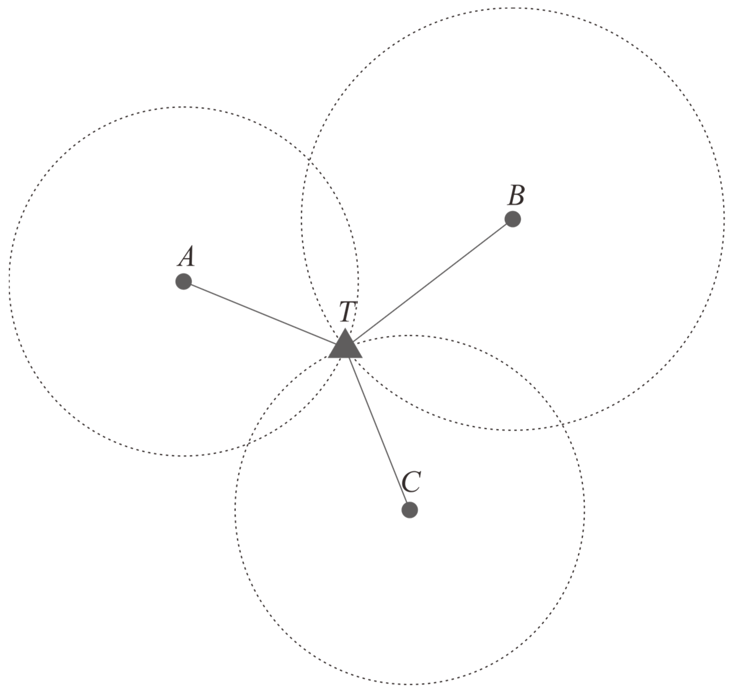
2.2.1. Base Station Location Technology Calculated by Distance

Distance-based localization techniques use geometrical relations to calculate the position of a measured object. The schematic diagram of the geometric triangle relationship is shown in Figure 1.

Equation (2) can be established using the position coordinates of the points A, B, and C at known locations and the distance between them and the measured point T. The position coordinates of the target point T can be obtained by solving the following equations:

$${(x_n-x_T)}^2+{(y_n-y_T)}^2=d_n{}^2,n=A,B,C$$

(2)

The distance between the target point and the known point can be estimated by the received signal strength indicator (RSSI). According to the experience of RSSI and propagation distance, there is Equation (3):

$$RSSI=P-10\alpha {\log }_{10}d$$

(3)

where $P$ represents the signal strength when the transmitting segment and the receiving end are separated by 1 m, and $\alpha$ represents the environmental attenuation factor. The value of $\alpha$ ranges from 2 to 3.5, with a smaller value in an open environment and a larger value in a closed environment with obstacles [25,26].

The distance calculation for the signal strength is affected by various factors such as the multipath signal, the inclination of the transmitted signal, and the signal propagation environment, so the results’ accuracy is not great. The distance can also be measured by time, which requires accurate time synchronization between the mobile terminal and the base station and is not suitable for network systems without clock synchronization, such as the Global System for Mobile Communications (GSM) and Universal Mobile Telecommunications System-Time Division Duplexing (UMTS-TDD). The round-trip delay can also measure the distance between the receiver and the base station. It does not require time synchronization, but it requires more network resources.

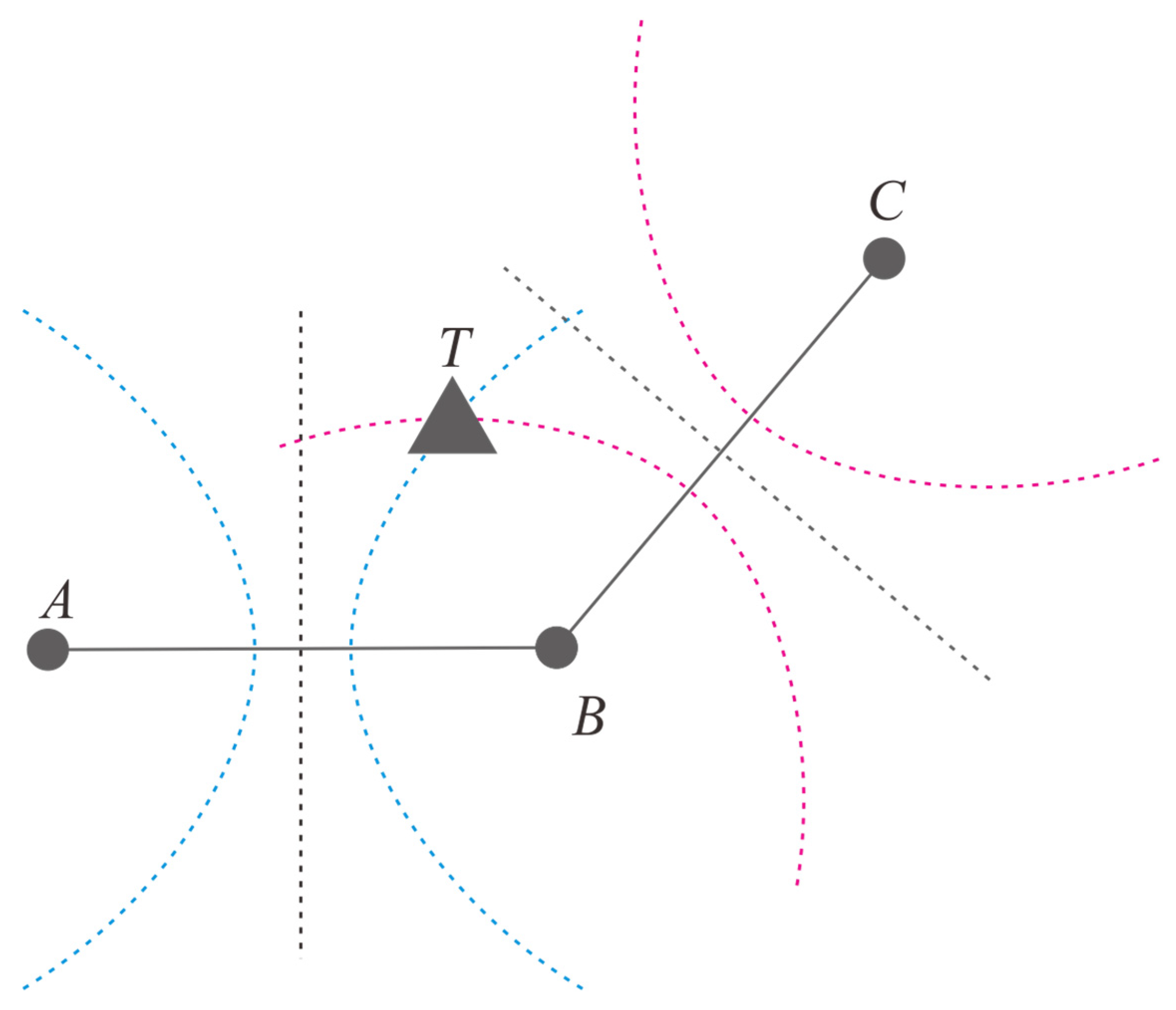
2.2.2. Base Station Location Technology Calculated by Time Delay

Base station location technology could also be calculated by the time delay of signal arrival. In this method, a hyperbola can be determined by using two base stations with known positions as the focal point and the difference in distance between the target point and the two base stations as the real axis length. When the target point can receive signals from three base stations, the two pairs of distance differences can be used to establish two hyperbolic equations, where the intersection of the two curves is the location of the target point. The geometric schematic of the method based on arrival time delay is shown in Figure 2.

The solution method based on time delay does not need the time synchronization of mobile terminals but only requires the time synchronization between base stations, which is more accurate and can be used in more network formats [27].

2.2.3. Based on the Origin Cellular Network Base Station Location

Origin cellular network localization is a proximity-based localization method. It determines the mobile terminal’s location based on the identification number, or Cell ID, of the station where the mobile terminal is located. It is the most widely used means of mobile terminal positioning, has no special requirements for mobile terminal devices, and can be applied to all network formats. Databases of mobile cellular network communication systems, such as the Home Location Register (HLR) or the Visiting Location Register (VLR), store the information of the Mobile Switching Center (MSC), where each mobile terminal is located. The location platform can obtain the location of the mobile terminal through the signaling exchange between the mobile terminal and the MSC. The localization method implemented by Cell ID has a short response delay. It produces stable and reliable results, but its localization accuracy depends on the density of base stations and is suitable for central urban areas [28].

2.3. GPS Location Assisted by Cellular Network

Satellite positioning has a long response time, requires quite good hardware devices to receive equipment, and the positioning results are affected by the environment. However, positioning methods based on base stations have poor positioning accuracy. The GPS positioning technology assisted by cellular networks complements both approaches to each other, resulting in more stable and accurate positioning results.

2.3.1. A-GPS

The A-GPS uses a rigid positioning GPS receiver to continuously track GPS satellites and transmit necessary satellite auxiliary information to mobile terminals. A-GPS uses the cellular network to assist the transmission of GPS signals, which makes GPS signals more stable and greatly reduces the time to first fix (TTFF) of the receiver [29].

2.3.2. GPS One

The GPS one method combines A-GPS, Advanced Forward Link Trilateration (AFLT) based on Code-Division Multiple Access (CDMA) networks, and the Cell ID position method. If the mobile terminal is in an open area and the number of satellites it can receive is greater than 4, GPS can be used for positioning. If the number of satellites that can be received is small, then the AFLT method based on the CMDA network or Cell ID method is used to locate the position according to the number of base station signals that can be received. Positioning methods based on combined satellite and base station data are also used in some cases. The GPS one method has a wide range of applications, providing more accurate location results and enhancing the availability of location services [30,31].

3. Travel Endpoint Identification Method: STDBSCAN

Mobile terminal devices generate a large amount of location information in the use of LBS services. These location points are arranged chronologically to form a sequence that can reflect the trajectories of the terminal device and the user. This sequence records the terminal equipment’s entire positional changes and contains the travel information. The relevant travel information can be estimated by analyzing the sequence, such as the orientation, destination, route, vehicle, motive, etc. The origin and destination of travel are the most critical data in the resident travel survey. This paper uses the spatial-temporal density-based spatial clustering of application with noise (STDBSCAN) method to extract the travel endpoints in the trajectory.

The density-based spatial clustering of application with noise (DBSCAN) method is a classical algorithm of the density-based clustering method [32,33]. It was presented at the 1996 Knowledge Discovery and Data Mining Conference. The DBSCAN is a density-based unsupervised spatial clustering algorithm. If the data points in an ellipsoidal space exceed a specific density, they are considered to form a particular class and search for their similar points. The method has two main parameters, $\mathrm{\epsilon }$ to control the size of the ellipsoid and minPts to bound the minimum number of data points in the ellipsoid space.

The trajectory data of the mobile terminal contain not only the spatial distance but also the time delay, which should be considered a different variable from the spatial distance. The STDBSCAN algorithm is an improvement on the DBSCAN. It adds a parameter $\Delta$ to control the time gap of points in the cluster so that the search range is changed from an ellipsoid to a cylindroid space [34].

In the travel identification of trajectory data, the parameters of the STDBSCAN model directly affect the clustering quality. Figure 3 shows a travel record of a trajectory identified by the STDBSCAN. $\mathrm{\epsilon }$ is related to the range of travel endpoints, which means the radius of the elliptic cylinder. $\Delta$ is related to the maximum residence time in a single trip, which means the height of the elliptic. minPt is related to parameters $\mathrm{\epsilon }$, $\Delta$, and the frequency of signaling exchange between the mobile terminal and MSC.

The whole STDBSCAN algorithm can be divided into two stages: cluster formation stage and cluster expansion stage:

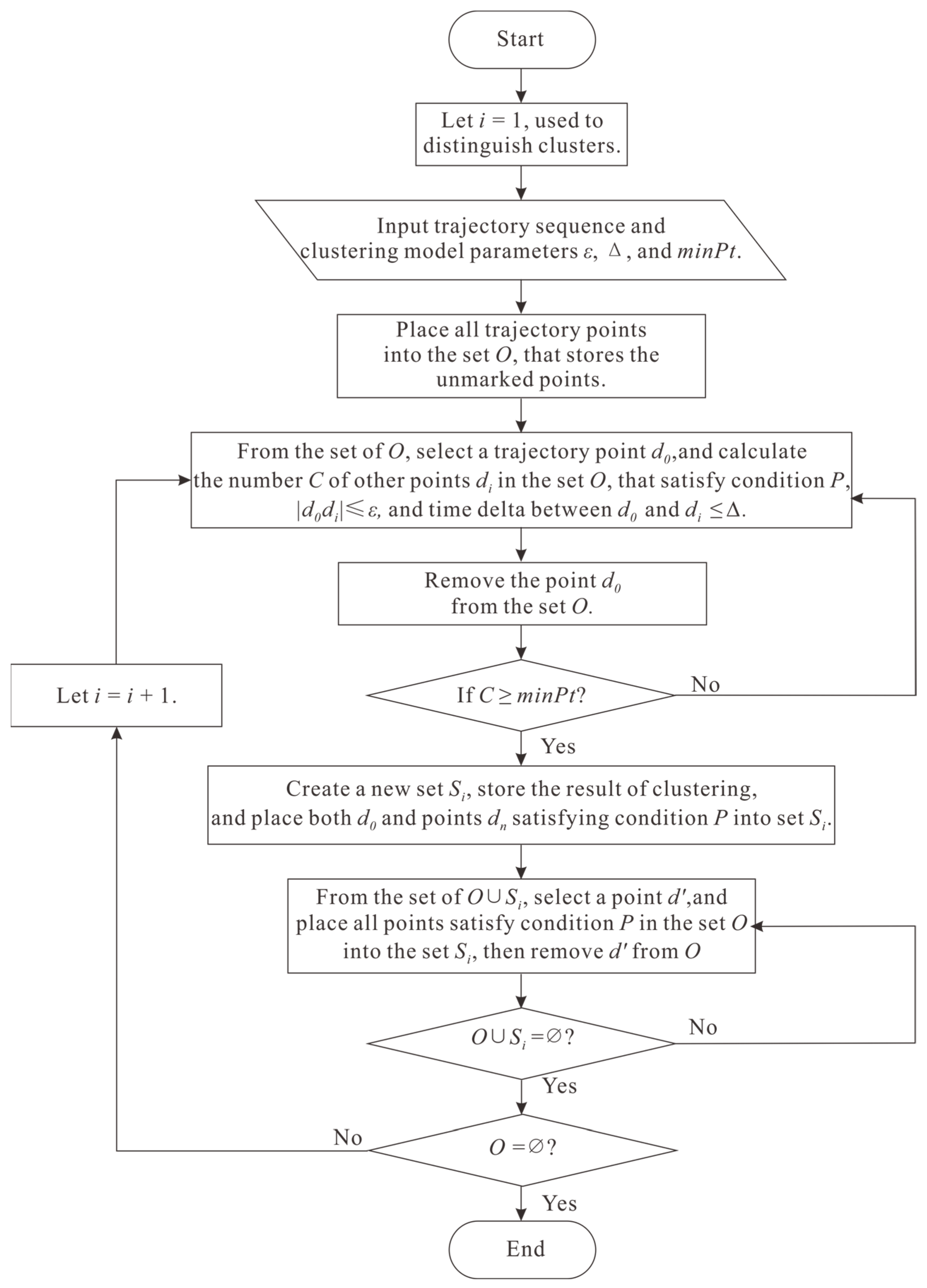
• At the beginning of the algorithm, all the location points are placed in the set $O$ representing unlabeled points, and then the cluster formation stage is entered.
• Cluster formation stage: randomly take a location point $d_0$ from the set $O$, and test whether it satisfies the condition $P$ for cluster formation. Regardless of whether the condition is satisfied, $d_0$ needs to be removed from the set $O$. If the condition $P$ is satisfied, the cluster expansion stage is entered; otherwise, the cluster formation stage is repeated.
• Cluster expansion stage: place all location points satisfying the condition $P$ into a cluster $S_i$, randomly find an unlabeled location point $d^{\prime }$ from $S_i$, and remove $d^{\prime }$ from the set $O$ at once. Then, all the points satisfying the condition $P$ for $d^{\prime }$ are added to $S_i$. This stage is repeated until there are no unlabeled points in $S_i$, and then the cluster formation stage is continued.
• When there are no location points in the set $O$, the whole algorithm ends.

The process of the STDBSCAN algorithm is shown in Figure 4, and the corresponding pseudocode is shown in Appendix A.

4. Experiment

This paper uses the STDBSCAN method to extract the travel endpoints from the travel trajectory data formed by cellular signaling data. The model parameters used in the experiment: minPts = 6, $\mathrm{\epsilon }$ = 0.075 km, and $\Delta$ = 300 s. The extracted results are applied to the study of travel origin–destination in transportation surveys, including the analysis of the spatial and temporal distribution of travel demand and travel volume and the study of the asymmetry of travel volume in different directions.

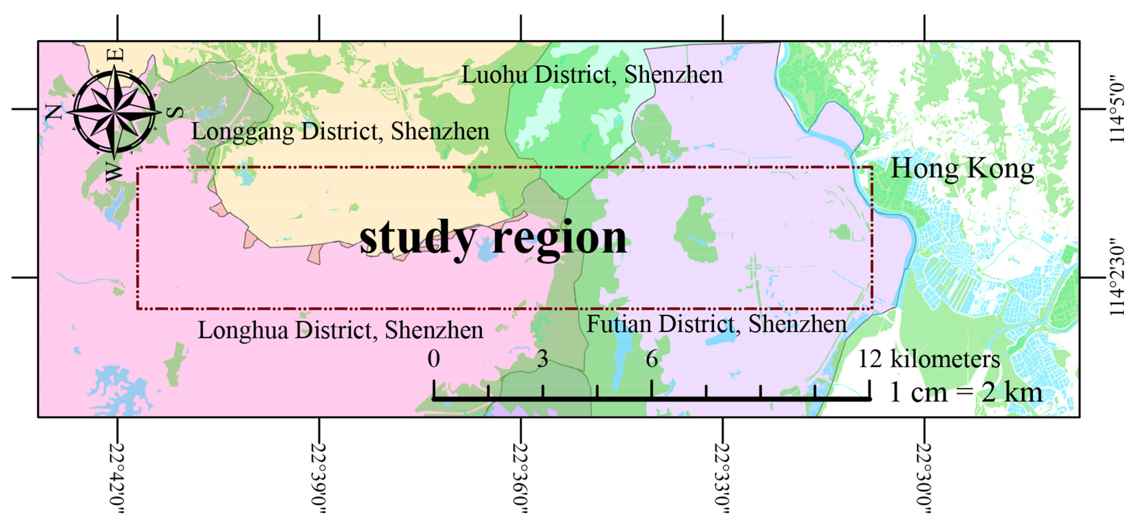
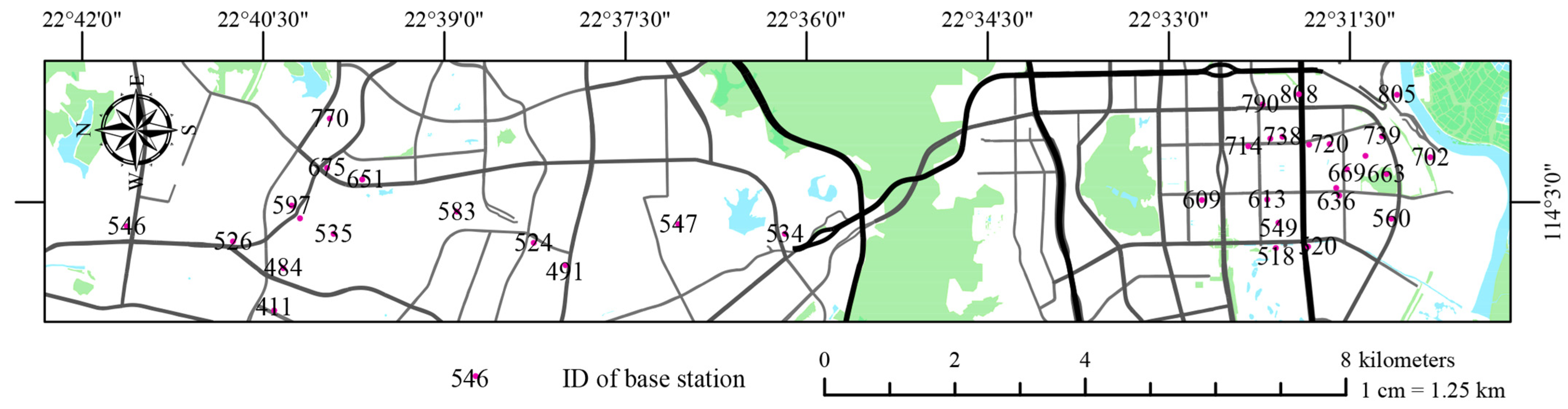
4.1. Study Region

The object of the study is cellular signaling data from 17:30 to 23:30 on 22 October 2013 in some areas of Shenzhen. The study area ranges from 114.034 to 114.069 in longitude and 22.513 to 22.695 in latitude and mainly involves Shenzhen’s Longgang District, Longhua District, and Futian District. The study region includes the natural environments of Tanglang Mountain Park and Silver Lake Mountain Park, which allows the study region to be divided into two traffic zones, and the trips within the study area can be roughly divided into three categories, including the travel within each traffic zone and the travel between the two zones. The geographical information of the study region, such as administrative divisions, road distribution, and natural environment, is derived from the data published by OpenStreetMap. The geographic information of the study region is shown in the following Figure 5.

4.2. Data Description and Preprocessing

This study uses cellular signaling data to identify urban travel origin and destination. Some examples of data are given below in

Table 1. Examples of cellular signaling data.

ID of SIM Card	Time	Longitude	Latitude
55555556	13:10:09	114.0397917	22.5740278
55555556	16:08:30	113.8056944	22.7613889
55555556	17:39:08	113.8090278	22.7561806
55555556	20:50:17	113.8465972	22.7725
55555556	23:53:07	114.0263889	22.6260417

. Within the study area, the dataset recorded a total of 5,599,176 records for 52,832 users or devices.

The first column indicates the ID of the SIM card. Due to the need for information security, it has no practical meaning and is only used to distinguish between different users. The second column is the time of the record, and the third and fourth columns indicate the location of the base station that was communicating with the user at the time. Some measures are used before the cluster analysis to improve the quality of the data. Conflicting data will be removed if multiple records exist for the same user simultaneously. If the number of records for a user is too low or the duration of the records is too short, all data for that user are removed. If there is data drift in the data arranged by time, this means the user’s mobile device switches communication with different base stations far away in a short period [35]. In that case, all data of that user will be removed.

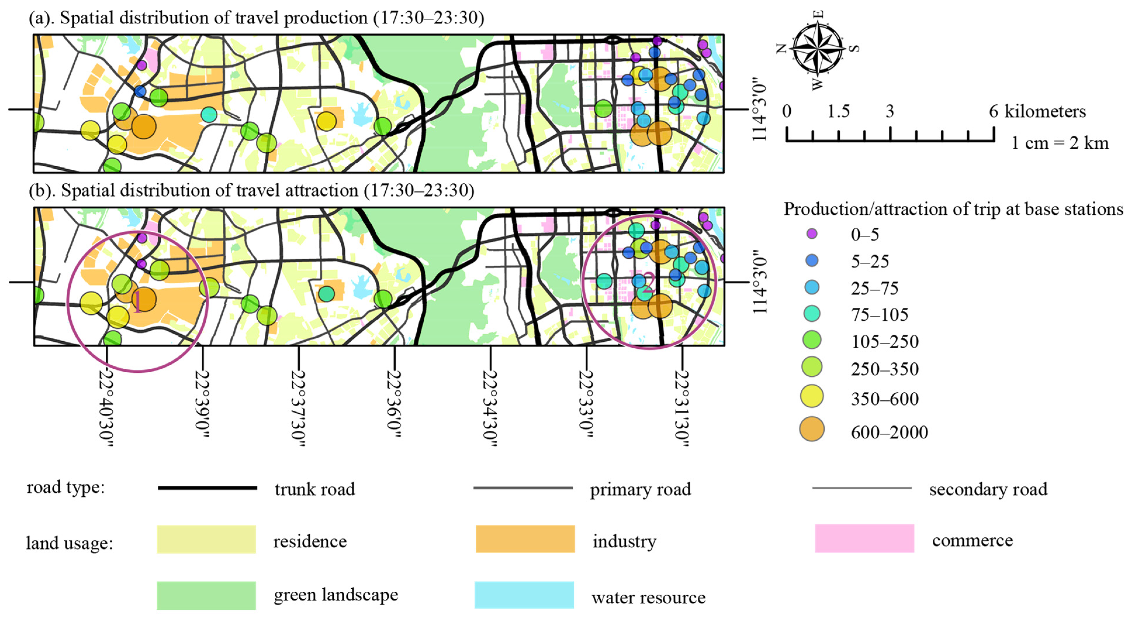
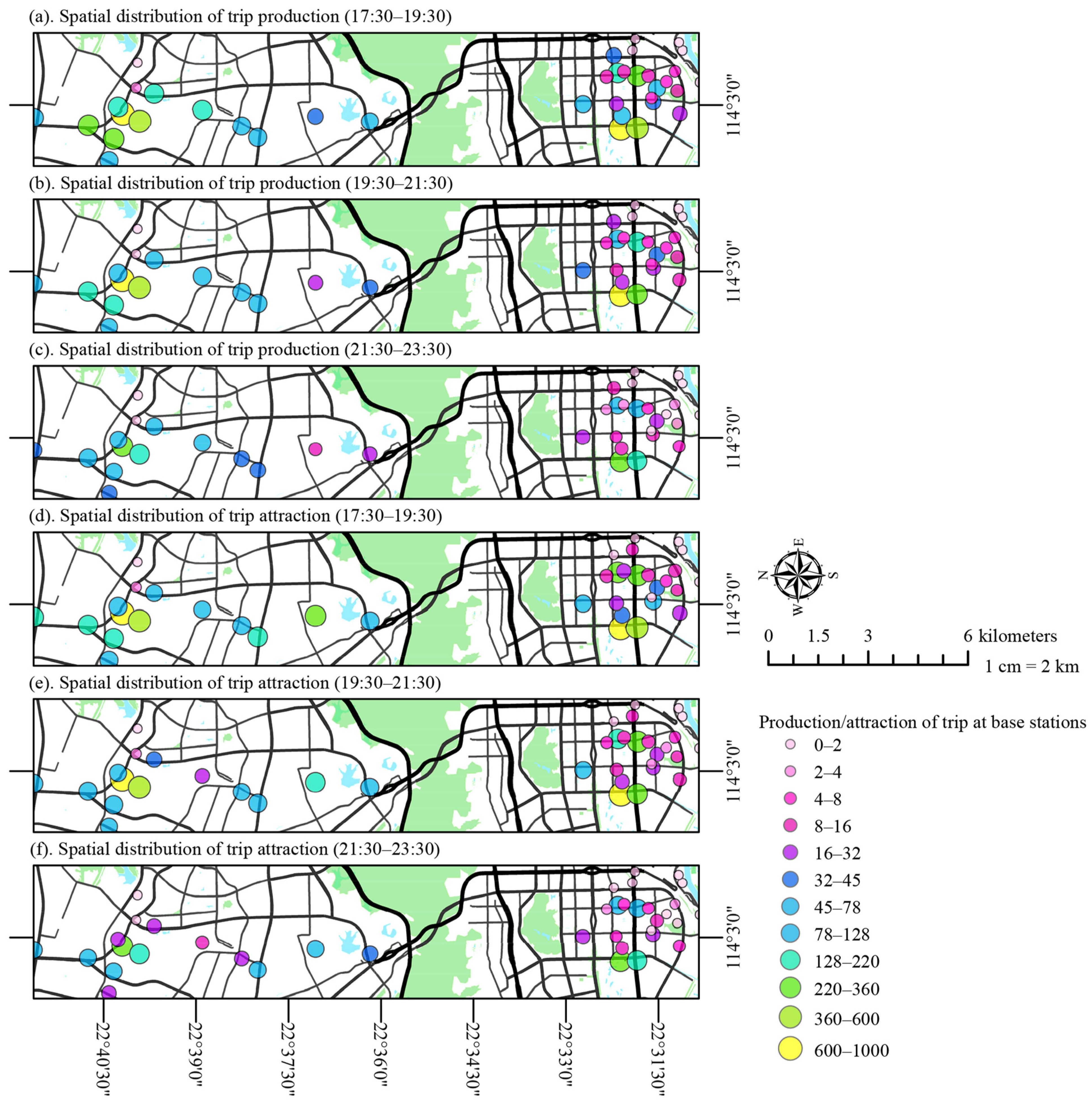
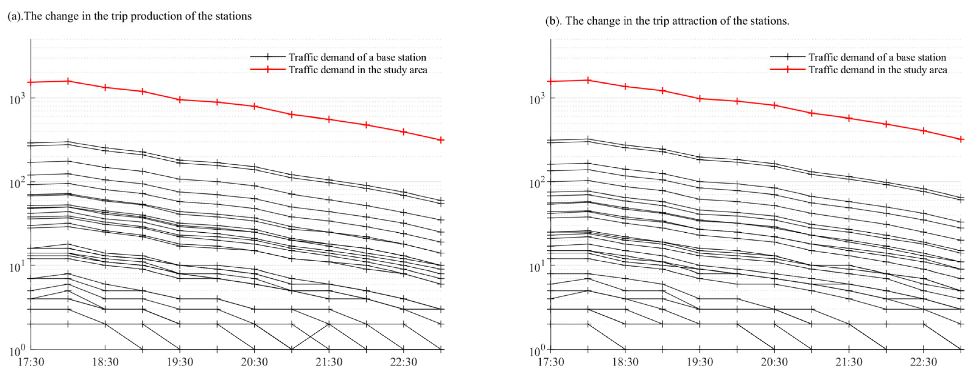
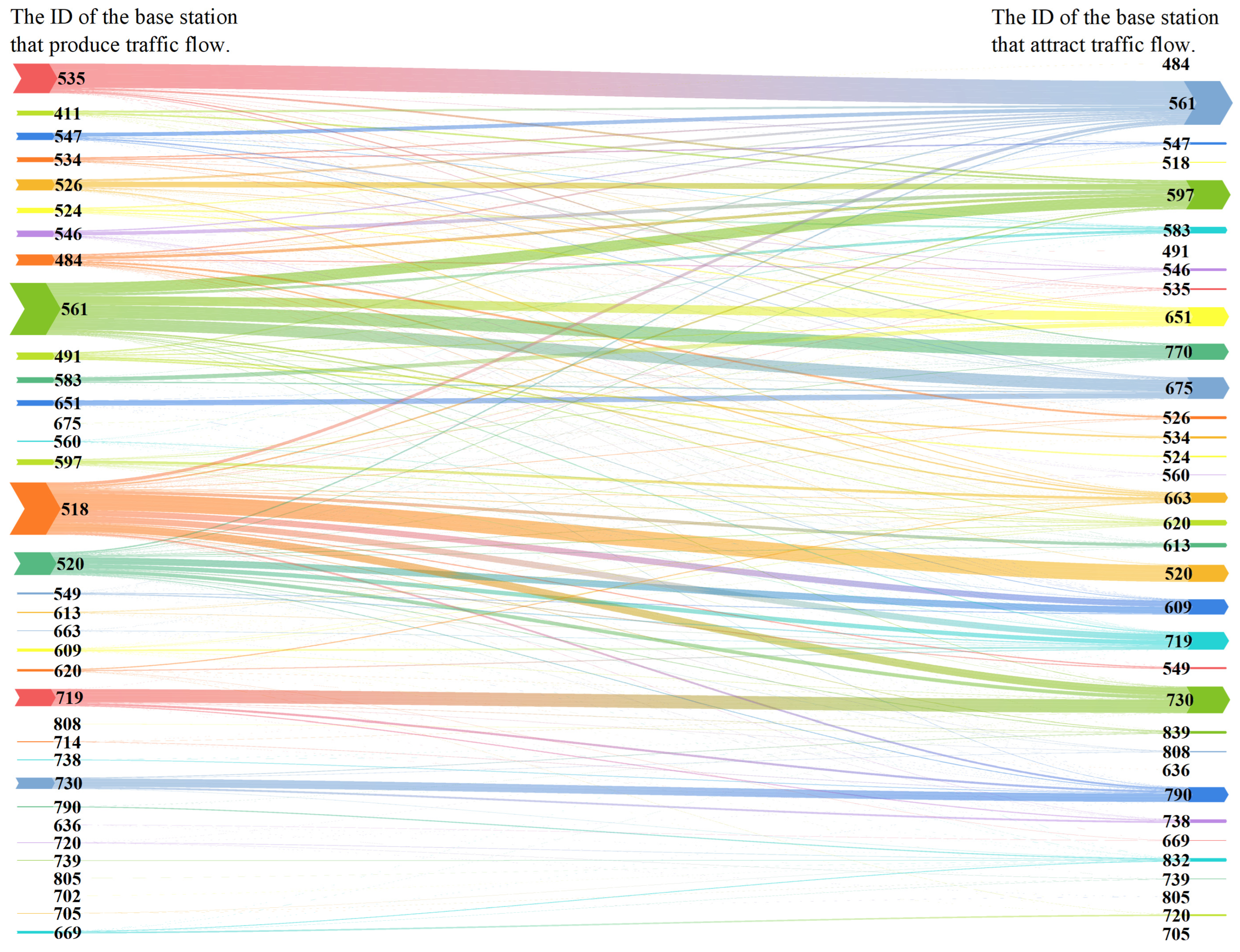
4.3. Distribution of Travel Demand

The STDBCAN method clusters cellular signaling trajectory data to obtain trip endpoints divided into origin and destination points. After that, the number of trip origin and destination points generated by each base station is counted as the amount of travel production and travel attraction, and the distribution of transportation demand graph is plotted in Figure 6.

The transportation demand of the study region fits the distribution of residential, industrial, and commercial areas and major roads in the city. Two main transportation demands are identified in Figure 6b. Region 1 is located in the industrial cluster of Longhua District, with many factories, such as Foxconn Technology Park. These factories attracted many workers, promoting the development of life service trades and creating many transportation demands. Region 2 is located in the Futian District, with commercial and cultural centers such as the Shenzhen Convention and Exhibition Center attracting many residents to travel.

The travel production and attraction at each station are calculated over half an hour to study the variation trend of travel demand over time, as shown in Figure 7.

According to Figure 7, after the evening traffic peak is over, the transportation demand at each station decreases to different levels, and the traffic production and attraction gradually decrease over time. To accurately reflect the changes in the number of traffic demands at each station, a logarithmic plot of the change in the travel production and attraction at each station over time is drawn in Figure 8. In Figure 8, each black line represents the change in the traffic volume of a base station, and the red line represents the change in the total traffic volume within the study area.

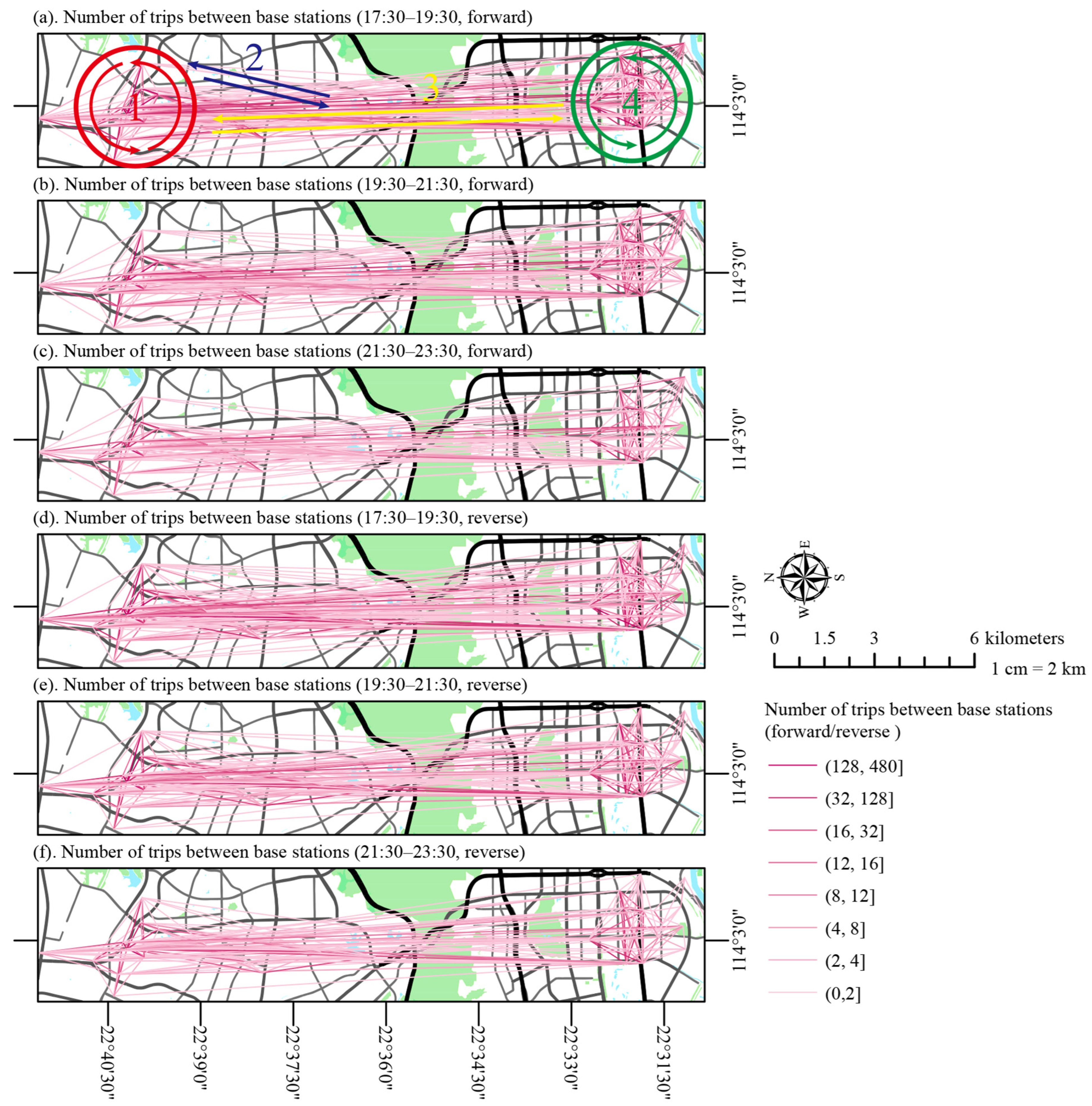
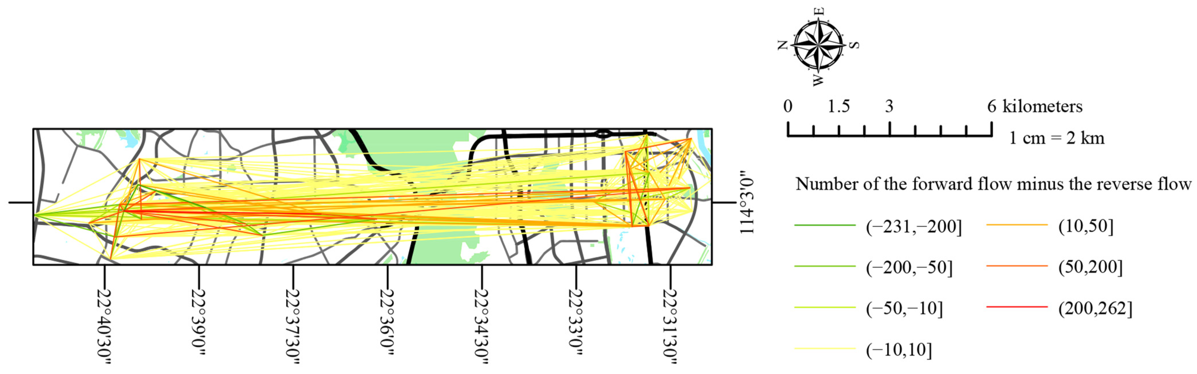
4.4. Traffic Flow Distribution and Travel Direction Asymmetry

Travel production and attraction statistics at different base stations can analyze the distribution of travel demand in time and space. Cellular signaling data can also be used to analyze the traffic intensity between two base stations. Figure 9 shows the traffic intensity between different base stations in the study area. In Figure 9, each line connecting the two base stations, named the desire line, represents the traffic intensity between the two base stations. The traffic flow between the two base stations has directivity, and this direction is affected by the structure of the urban road network, which is predominantly north–south. Thus, the trip from the northern base station to the southern base station is defined as a forward direction. Otherwise, it is defined as a reverse direction.

The travel intensity between different base stations can reflect the distribution of travel demand in time and space. Similar to the analysis result of traffic production and attraction, the traffic demand in the study area is mainly generated by the corporate park in Longgang District and the commercial and cultural center in Futian District, and the travel demand decreases gradually with the fall of night. Four major traffic flows are marked in Figure 9a. Mark 1 represents the travel within the industrial area, Mark 2 represents the travel between the industrial area and the nearby residential area, Mark 3 represents the travel between the industrial area and the commercial and cultural center, and Mark 4 represents the travel within the commercial center.

In the research and practice of transportation planning, the desire line is a common means to show the traffic intensity. However, when many transportation zones are involved in the study area, the overlap and coverage of expected lines can cause reading difficulties. Figure 9 does not focus on showing the specific value of a particular expected line, but rather on the distribution of the overall traffic intensity in the city. To better show the numerical differences in traffic intensity between stations, Figure 10 and Figure 11 are drawn. In Figure 10, the ID of the base station in the research area is marked, and in Figure 11, the Sankey diagram of the traffic intensity between base stations in the period from 17:30 to 23:30 is shown.

In order to understand the traffic asymmetry between different stations, the difference between forward flow and reverse flow is calculated, and Figure 12 is drawn.

According to Figure 12, the traffic asymmetry in the study region is mainly generated by the traffic flow leaving the corporate park. Some traffic management policies can be implemented to alleviate this traffic asymmetry, such as taxi dispatch and assigning shared bikes.

4.5. Results

The travel origin and destination points obtained from the cellular signaling data processed by the STDBSCAN can explain the distribution of urban traffic demand, the correlation degree between different traffic zones, and the asymmetry of traffic flows well. Different from the traditional travel data obtained via household interviews, cellular signaling data are passively acquired. This analysis method does not require long-term survey preparation or a large staff and can be carried out over a long period with a low cost to achieve timely feedback on urban traffic demand.

5. Conclusions

A low-cost, timely, and durable long-term approach to resident travel surveys is crucial for urban transportation planning and traffic management. This paper uses the STDBSCAN method to identify travel endpoints of cellular signaling trajectory data and analyze travel demand and travel characteristics in the studied region. The results show that the location information generated by mobile internet terminals can be applied to the study of urban traffic with the advantages of low survey costs, timely feedback, and long-term fulfillment.

This study considers that the location information generated by mobile internet terminals plays an essential role in urban transportation research and can supplement conventional resident travel surveys. But there is still a lot to look at in the use of location information.

• In this paper, the signaling data collected by the Cell ID method are used in the experiment. Although the Cell ID method is widely used in practical applications, its localization results are not spatially continuous. This means that the clustering results will be affected by the base station density, and if the number of base stations is too small, the STDBSCAN method may not work properly. More types of positioning data, which use more diverse positioning techniques, may achieve better results. All trajectory data belong to the spatial coordinate permutation formed by time order, which is consistent in the data format, so the STDBSAN method can work well with these data types. These data have different characteristics due to their different localization techniques. More research is needed on exploiting data characteristics and achieving better results in the application domains when using location information from different positioning technologies.
• The STDBSCAN method uses two parameters, $\mathrm{\epsilon }$ and $\Delta$, that control the spatial and temporal variables, respectively, which makes it very interpretable when dealing with spatial problems in time series. In the experiment of this study, the travel origin and destination points obtained from the cellular signaling data processed by the STDBSCAN can explain the distribution of urban traffic demand, the correlation degree between different traffic zones, and the asymmetry of traffic flows well. However, there is not only one way to identify travel behavior from trajectory sequences. More clustering methods, judgment rules, or more advanced methods may perform better when dealing with location information sequences.
• This paper has identified travel endpoints from cellular signaling data. It analyzed the distribution of urban travel demand in time and space, the traffic correlation between different traffic areas, and the asymmetry of traffic flow in different travel directions. More travel characteristics may be obtained via further analysis of cellular signaling data. For example, the travel path can be estimated through trajectory points during the travel process, and the travel speed can be calculated by calculating the data of each trajectory point during the travel process to estimate the travel mode. In addition to the traffic field, the location information generated by mobile networks represented by cellular signaling data could be applied to more diverse research fields.

References

- Li, J.Z.; Li, W.Y.; Lian, G. Optimal Aggregate Size of Traffic Sequence Data Based on Fuzzy Entropy and Mutual Information. Sustainability 2022, 14, 14767. [Google Scholar] [CrossRef]
- Li, J.Z.; Li, W.Y.; Lian, G. A Nonlinear Autoregressive Model with Exogenous Variables for Traffic Flow Forecasting in Smaller Urban Regions. Promet-Zagreb 2022, 34, 943–957. [Google Scholar] [CrossRef]
- Giles-Corti, B.; Vernez-Moudon, A.; Reis, R.; Turrell, G.; Dannenberg, A.L.; Badland, H.; Foster, S.; Lowe, M.; Sallis, J.F.; Stevenson, M.; et al. City planning and population health: A global challenge. Lancet 2016, 388, 2912–2924. [Google Scholar] [CrossRef] [PubMed]
- Nieuwenhuijsen, M.J. Urban and transport planning pathways to carbon neutral, liveable and healthy cities; A review of the current evidence. Environ. Int. 2020, 140, 105661. [Google Scholar] [CrossRef]
- Young, M.; Farber, S. The who, why, and when of Uber and other ride-hailing trips: An examination of a large sample household travel survey. Transp. Res. Part A Policy Pract. 2019, 119, 383–392. [Google Scholar] [CrossRef] [Green Version]
- An, S.; Yang, H.; Wang, J. Revealing Recurrent Urban Congestion Evolution Patterns with Taxi Trajectories. ISPRS Int. J. Geo-Inf. 2018, 7, 128. [Google Scholar] [CrossRef] [Green Version]
- Pineda-Jaramillo, J.; Arbelaez-Arenas, O. Assessing the Performance of Gradient-Boosting Models for Predicting the Travel Mode Choice Using Household Survey Data. J. Urban Plan. Dev. 2022, 148, 04022007. [Google Scholar] [CrossRef]
- Ji, Y.J.; Cao, Y.; Liu, Y.; Guo, W.H.; Gao, L.P. Research on classification and influencing factors of metro commuting patterns by combining smart card data and household travel survey data. Iet Intell. Transp. Syst. 2019, 13, 1525–1532. [Google Scholar] [CrossRef]
- Stopher, P.R.; Kockelman, K.; Greaves, S.P.; Clifford, E. Reducing Burden and Sample Sizes in Multiday Household Travel Surveys. Transp. Res. Rec. 2008, 2064, 12–18. [Google Scholar] [CrossRef] [Green Version]
- Choi, J.; Lee, W.D.; Park, W.H.; Kim, C.; Choi, K.; Joh, C.H. Analyzing changes in travel behavior in time and space using household travel surveys in Seoul Metropolitan Area over eight years. Travel. Behav. Soc. 2014, 1, 3–14. [Google Scholar] [CrossRef]
- Liu, Y.W.; Cirillo, C. Small area estimation of vehicle ownership and use. Transp. Res. Part D Transp. Environ. 2016, 47, 136–148. [Google Scholar] [CrossRef] [Green Version]
- Federal Highway Adminnistration Office of Policy Information. 2017 NHTS Data User Guide. Available online: https://nhts.ornl.gov/assets/NHTS2017_UsersGuide_04232019_1.pdf (accessed on 1 April 2023).
- Christie, S.; Keyes, A.; Swannell, B.; Templeton, I.; Mann, J. National Travel Survey 2021 Technical Report. Available online: https://assets.publishing.service.gov.uk/government/uploads/system/uploads/attachment_data/file/1103925/nts-technical-report-2021.pdf (accessed on 1 April 2023).
- Department for Transport. Road Use Statis Great Britain. 2016. Available online: https://assets.publishing.service.gov.uk/government/uploads/system/uploads/attachment_data/file/514912/road-use-statistics.pdf (accessed on 1 April 2023).
- Department for Transport. Cycling and Walking Investment Strategy. 2017. Available online: https://assets.publishing.service.gov.uk/government/uploads/system/uploads/attachment_data/file/918442/cycling-walking-investment-strategy.pdf (accessed on 1 April 2023).
- Department for Transport. Rail Demand Forecasting Estimation. Available online: https://assets.publishing.service.gov.uk/government/uploads/system/uploads/attachment_data/file/610059/phase2-rail-demand-forecasting-estimation-study.pdf (accessed on 1 April 2023).
- Department for Transport. National Travel Survay—Why people travel: Shopping. 2015. Available online: https://assets.publishing.service.gov.uk/government/uploads/system/uploads/attachment_data/file/604103/why-people-travel-shopping-2015.pdf (accessed on 1 April 2023).
- Department for Transport. National Travel Survey 2014: Travel to School. 2014. Available online: https://assets.publishing.service.gov.uk/government/uploads/system/uploads/attachment_data/file/476635/travel-to-school.pdf (accessed on 1 April 2023).
- Department for Transport. National Travel Survey: Motorcycle Use in England. 2016. Available online: https://assets.publishing.service.gov.uk/government/uploads/system/uploads/attachment_data/file/694965/motorcycle-use-in-england.pdf (accessed on 1 April 2023).
- Barbosa, H.; Barthelemy, M.; Ghoshal, G.; James, C.R.; Lenormand, M.; Louail, T.; Menezes, R.; Ramasco, J.J.; Simini, F.; Tomasini, M. Human mobility: Models and applications. Phys. Rep.-Rev. Sec. Phys. Lett. 2018, 734, 1–74. [Google Scholar] [CrossRef]
- Yang, Y.; Xie, X.; Fang, Z.; Zhang, F.; Wang, Y.; Zhang, D. VeMo: Enabling Transparent Vehicular Mobility Modeling at Individual Levels with Full Penetration. IEEE Trans. Mob. Comput. 2022, 21, 2637–2651. [Google Scholar] [CrossRef]
- Hussain, S.A.; Hassan, M.U.; Nasar, W.; Ghorashi, S.; Jamjoom, M.M.; Abdel-Aty, A.H.; Parveen, A.; Hameed, I.A. Efficient Trajectory Clustering with Road Network Constraints Based on Spatiotemporal Buffering. Isprs Int. J. Geo-Inf. 2023, 12, 117. [Google Scholar] [CrossRef]
- Boeing, G.; Higgs, C.; Liu, S.; Giles-Corti, B.; Sallis, J.F.; Cerin, E.; Lowe, M.; Adlakha, D.; Hinckson, E.; Moudon, A.V.; et al. Using open data and open-source software to develop spatial indicators of urban design and transport features for achieving healthy and sustainable cities. Lancet Glob. Health 2022, 10, e907–e918. [Google Scholar] [CrossRef] [PubMed]
- Long, Y.; Thill, J.C. Combining smart card data and household travel survey to analyze jobs-housing relationships in Beijing. Comput. Environ. Urban 2015, 53, 19–35. [Google Scholar] [CrossRef] [Green Version]
- Shi, Y.; Shi, W.; Liu, X.; Xiao, X. An RSSI Classification and Tracing Algorithm to Improve Trilateration-Based Positioning. Sensors 2020, 20, 4244. [Google Scholar] [CrossRef]
- Qu, Z.J.; Liu, C.; Zeng, H.; Gao, T.Z.; Xu, J.; Liu, H.X. A Method for Locating Tools in the Railway Moving Area Optimized Based on Received Signal Strength Indicator and a Fuzzy Neural Network. IEEE Sens. J. 2021, 21, 23185–23197. [Google Scholar] [CrossRef]
- Li, W.C.; Zhang, T.; Li, F.; Wang, Z.L.; Ni, T.; Fan, X.J.; Shi, Y. Location Performance Test and Evaluation for Tri-Station Time Difference of Arrival System. J. Commun. Technol. Electron. 2021, 66, S175–S184. [Google Scholar] [CrossRef]
- Lv, M.Q.; Zeng, D.J.; Chen, L.; Chen, T.M.; Zhu, T.T.; Ji, S.L. Private Cell-ID Trajectory Prediction Using Multi-Graph Embedding and Encoder-Decoder Network. IEEE Trans. Mob. Comput. 2022, 21, 2967–2977. [Google Scholar] [CrossRef]
- Kong, S.H. High Sensitivity and Fast Acquisition Signal Processing Techniques for GNSS Receivers. IEEE Signal Proc. Mag. 2017, 34, 59–71. [Google Scholar] [CrossRef]
- Kong, S.H. Fast Multi-Satellite ML Acquisition for A-GPS. IEEE Trans. Wirel. Commun. 2014, 13, 4935–4946. [Google Scholar] [CrossRef]
- del Peral-Rosado, J.A.; Raulefs, R.; Lopez-Salcedo, J.A.; Seco-Granados, G. Survey of Cellular Mobile Radio Localization Methods: From 1G to 5G. IEEE Commun. Surv. Tutor. 2018, 20, 1124–1148. [Google Scholar] [CrossRef]
- Sarteshnizi, I.T.; Sarvi, M.; Bagloee, S.A.; Nassir, N. Temporal pattern mining of urban traffic volume data: A pairwise hybrid clustering method. Transp. B Transp. Dyn. 2023, 11, 2185496. [Google Scholar] [CrossRef]
- Kremers, B.J.J.; Citrin, J.; Ho, A.R.; van der Plassche, K. Two-step clustering for data reduction combining DBSCAN and k-means clustering. Contrib. Plasma Phys. 2023, 63, e202200177. [Google Scholar] [CrossRef]
- Wang, P.X.; Wu, S.; Zhang, H.C.; Lu, F. Indoor Location Prediction Method for Shopping Malls Based on Location Sequence Similarity. Isprs Int. J. Geo-Inf. 2019, 8, 517. [Google Scholar] [CrossRef] [Green Version]
- Quang, B.V.; Prasad, R.V.; Niemegeers, I. A Survey on Handoffs—Lessons for 60 GHz Based Wireless Systems. IEEE Commun. Surv. Tutor. 2012, 14, 64–86. [Google Scholar] [CrossRef]