Article

Exploring the Correlation between Streetscape and Economic Vitality Using Machine Learning: A Case Study in the Old Urban District of Xuzhou, China

School of Architecture and Design, China University of Mining and Technology, Xuzhou 221116, China
*
Author to whom correspondence should be addressed.
ISPRS Int. J. Geo-Inf. 2023, 12(7), 267; https://doi.org/10.3390/ijgi12070267
Submission received: 1 June 2023 / Revised: 19 June 2023 / Accepted: 29 June 2023 / Published: 4 July 2023

Abstract

:
The streetscapes of old urban districts record the changes in urban space and the vitality of socio-economic entities like storefronts. However, prior studies of urban vitality have preferred the demand end of crowd agglomeration to the supply end of commercial businesses, while the refined application of street-view images (SVIs) and the spatial heterogeneity resulting from sectional differences among elements deserve further research. Under this context, this paper took both the alive and the closed storefronts as the objects and developed an analytical framework based on machine learning and SVIs to analyze the characteristics of the streetscape and the economic vitality, followed by a regression analysis between them with a multiscale geographically weighted regression (MGWR) model. Our findings comprise three aspects: (1) despite the sum of the storefronts being more often used, combining the alive and the closed businesses is beneficial to reflect the real economic vitality; (2) as a reflection of the spatial heterogeneity and sectional differences of elements, the asymmetric streetscape has a significant influence on the economic vitality; and (3) although different factors from the streetscape can influence economic vitality differently, based on varied proxies of the vitality, three factors, namely, higher difference value of the signboards, higher sum of glass interfaces, and lower difference value of the glass interfaces, can benefit the economic vitality. This research can support urban physical examination and the regeneration of old urban districts for urban planners, designers, and decision-makers, and provide new perspectives and proxies as well as a more fine-grained analysis among the traditional studies on economic vitality.

1. Introduction

As the witnesses of urban civilization, the streetscapes of old urban districts record the changes of urban streets and storefronts, which provide places for the interaction of economic, social, political, and cultural activities [1]. They also represent the urban character and collective memory of the local residents [2,3]. With most of the old streets located in the cores of the cities, however, long-term, high-intensity consumption of materials and limited incremental land resources, combined with urban expansion and suburbanization, have made many of them the pain points of the cities. Actually, it is not just a problem of the linear streets, but the whole urban area. Decreased population, vacant buildings, deteriorated living standards, precarious infrastructure, and fragile economic environments, as well as lack of vitality, are all representative of many old urban districts around the world [4,5,6,7,8]. Considering both the value of and the challenge facing old urban districts, how to efficiently and accurately target the issue and then help solve it deserves in-depth research.
Under the framework of the Sustainable Development Goals (SDGs) released by the United Nations [9], many efforts have been taken during the regeneration of old urban districts. On the one hand, many scholars focus on the topics like urban politics, governance policy, institutional roles, community initiatives, and retail economy to promote complicated social and economic interactions [10,11,12,13]. Particularly, retail, as an approach to urban regeneration, has raised much attention in recent years [1,14,15,16]. With the transformation of the role of old urban districts from production to consumption [14], cultivating a vibrant retail sector in such areas can not only create jobs, increase taxation, and meet the everyday needs of the locals, but also beautify the urban image and attract tourists. Under the context of fine governance and the awareness of the “human-centered” concept, numerous small and medium-sized retail stores related to people’s livelihood act as a lively reflection of social reality and economic vitality. On the other hand, the question of how to attach different urban visions to the physical urban space has been explored from the perspectives of morphology, urban vitality, and so on [3,5,17,18,19].
In the research field of urban vitality, there are fixed names of pioneers that are often cited, such as Jacobs (1961), Gehl (1971), Lynch (1981), Whyte (1980), Maas (1984), Montgomery (1998), Katz et al. (1994), etc. [20,21,22,23,24,25,26]. Because of the overlapping with the name list of famous urban morphologists, it is not surprising that many studies are conducted in order to analyze the relationship between indexes of the built environment and urban vitality, with the spatial scale ranging from a land grid of 1 km by 1 km to an alley [27,28,29,30,31,32,33,34,35,36,37,38]. In fact, how to interpret “vitality” has had significant influence on later research. As many scholars have mentioned, the concept of “vitality” seems relatively easy to observe but difficult to define. Until now, it has been reflected by smart card data, night-time light data, social media check-in data, Baidu heat map data, video data, location-based services (LBS) data, point-of-interest (POI) data, small catering data, etc.
Although the approaches are diverse, there are still some aspects to be improved. First, despite different comprehension and tools, most of the traditional studies focus on the demand end rather than the supply end to represent urban vitality. In other words, the studies pay more attention to describing and measuring the agglomeration of people, but few studies attempt to understand the role of the service providers, especially the ordinary socio-economic entities along the road, in providing and maintaining urban vitality. After all, it is the storefronts that create a relatively stable economic environment and streetscape in urban areas. Second, traditional measurement of sky, greenery, roads, and building facades is still mainstream in the application of SVIs, especially in vitality-related research. Meanwhile, there is a trend of advanced exploration of the data in a creative and refined way, including classifying the details of interfaces and commercial brands of the storefronts. Third, although the analytical scale varies, the street segment is widely accepted as the unit of urban governance and spatial intervention. However, the spatial heterogeneity resulting from the sectional differences in the values of the indexes and its influence on the vitality have rarely been studied. Actually, in order to reach such precision, a smaller scale than that of the street segment is required.
To the best of our knowledge, there have been few studies focusing on common storefronts that depict the features of their interface elements and reveal the economic vitality directly based on the machine learning technique and SVIs. Among the related literature, we have noticed that some scholars have conducted partially similar studies. For instance, Tsai et al. (2014) proposed a dataset of “on-premise signs” and developed a framework to recognize commercial signs using SVIs [39]. Ye et al. (2019) combined SVIs and deep learning to analyze the urban commerce distribution [40]. Zamir et al. (2011) attempted to identify commercial entities using a text detection algorithm [41]. Despite their inspiration for our research, commercial signage or signs are what they mainly focus on, with other elements of the streetscape such as doors and windows, the condition of businesses, and the relationship between physical features and economic vitality behind the SVIs not mentioned. In view of the existing literature, our research takes a step further mainly in three aspects: (1) the objects to represent economic vitality are enriched from two perspectives of both the alive and the closed businesses; (2) a set of proxies is developed totally from SVIs to measure the characteristics of the streetscape and the effects on economic vitality from the scales of street segment and point, respectively; and (3) the spatial heterogeneity reflected by the sectional differences of the elements is analyzed in a fine-grained way. For these purposes, using machine learning and SVIs, we take the ordinary storefronts as the objects and set up a series of proxies to measure the economic vitality from two perspectives of both the alive and the closed businesses, as well as the related characteristics of the streetscape, followed by a regression analysis between economic vitality and the characteristics of the streetscape with an MGWR model.

2. Literature Review

2.1. Economic Vitality and Its Measurement

Due to the aforementioned ambiguous definition of “vitality”, the concept has been talked about in many different contexts. Some scholars attempt to evaluate it in a comprehensive way, including social, economic, and cultural interpretations [28,42], while in some research, the pedestrian activity or flow volume, which can be classified into the social dimension in Maas’ words [24], is regarded as representative [19,29,43,44]. In addition, certain spatial indexes of the urban environment are also added to represent vitality in other studies. Based on the diversified connotations, in our study, the ordinary small- and medium-sized storefronts were deemed as reflective of economic vitality.
Economic vitality is actually an inherent part of urban vitality, especially from the significant but seemingly inconspicuous storefronts. As is known to us all, Jacobs (1961) is thought to be the first master to have paid attention to diversity and vitality. In her discourse about Wall Street in Manhattan, for instance, the retail sector and catering businesses that were under decay were related closely to the depression of street life [20]. Furthermore, in Maas’ doctoral thesis, a variety of individual-owned shops that provide kinds of goods and services for the city are of great significance as the economic components of urban vitality [24]. From these works, along with other traditional research works, we can conclude that ordinary storefronts should be regarded as components in a vibrant street and city life, apart from the gathering of pedestrian and their diversified activities.
With the progress of technologies and tools, recent studies have been conducted using quantitative measurements. Among the literature, Long and Huang (2017) is an example of explicitly focusing on economic vitality, and they use data covering hundreds of cities and analyze them in geographical units of 1 km by 1 km [34]. Actually, based on obscure and generalized definitions of urban vitality, more studies apply small catering business and restaurant data as a proxy for measuring the economic vitality from a third-party platform like Dianping (https://www.dianping.com/, access on 19 June 2023). Therefore, we focused on the content about economic vitality and collected some of them in Table 1 [5,27,32,33,34,42,45,46]. In addition, there are extensive studies that pay attention to retail stores and restaurants under the context of economic geography. Some representatives are also listed in Table 1 [47,48,49]. Despite their different study area and spatial scale, however, there are two problems to be improved. First, considering that the records of different shops like POIs from big data platforms are usually renewed slowly, the real state of them is questionable due to the changing of businesses and other reasons [40]. Second, proxies like small catering businesses and restaurants cannot cover all the small and medium-sized shops along urban roads. Particularly, in dense urban areas like old urban districts, some shops are mixed with the homes of the local residents in the communities, which are not seen from the public urban streets. With the development of SVI and related technologies, these problems can be further explored.

2.2. Streetscape and Machine Learning

Using images or videos to investigate urban space and record spatial change has a long history. Compared to abstract models and statistical results, it is more intuitive and enables abundant on-site experience. While traditional field surveying is widely utilized [50], more and more of the latest studies have relied on SVIs from Google Street View, Baidu Street View, Tencent Street View, etc., as a complement to satellite-based images [51] to reduce their labor and time costs. Moreover, wearable devices and sensors can also be used to capture images of certain spaces [37,43].
The widespread use of SVIs closely connects to the application of machine learning algorithms, such as DeepLab [35,38], ResNet [31], FCN [36], SegNet [43], and YOLO [52]. In some studies, several kinds of models are used together [29]. Among the existing literature, however, the green view index, sky view index, pavement index, as well as building frontage index are still the main concerns, based on the relatively mature pre-trained models. At the same time, apart from traditional calculation of the elements of the built environment, some scholars have attempted to reveal deeper connotations and correlations behind the SVIs. For example, Tsai et al. (2014) identified on-premise signs as a potential method to recognize different shops [39]. Ye et al. (2019) analyzed the distribution of urban commerce through taking storefronts’ signage as a kind of commercial facility [40]. Furthermore, in two scientific reports, Palmer et al. (2021) identified and classified unhealthy outdoor advertisements to explore their influence on social inequalities [53], while Suel et al. (2019) attempted to measure inequalities of income, education, crime, living environment, and some other social indexes directly through SVIs without intermediate processes [54]. Following this trend, we aim to extend the scope of the application of SVIs and reveal more information about the storefronts behind the images.

3. Materials and Methods

To verify our idea, an empirical study was conducted in the old urban district in Xuzhou, China. After an overview about the study area, several steps of data acquisition and processing were introduced, with ordinary storefronts as the objects. An analytical framework was developed based on machine learning and SVIs to analyze the characteristics of the streetscape and the economic vitality behind the images, followed by a correlation analysis between them with an MGWR model. Finally, a series of dependent and independent variables and their descriptions were defined in the last sub-section, as well as the calculation methods.

3.1. Study Area

This study focuses on the old urban district of Xuzhou (see Figure 1), an eastern Chinese city in Jiangsu Province. For approximately 2600 years of city construction, the old urban district in Xuzhou has maintained its core for a long time (see Figure 2) and gradually expanded outward in a circular manner [55]. Although the establishment and development of the new urban district located to the east has attracted much attention and financial support, the old urban district has its own advantages, with many residents still living in it. According to the latest Territorial and Spatial Master Plan of Xuzhou (2021–2035), the old urban district should take the role of the center within the central area [56]. Under the framework of acts of urban regeneration, it can grasp the opportunity to improve urban quality and vitality. At the same time, however, the district confronts complex challenges including a decayed environment of neighborhoods, chaotic street order, and obscure urban character. Therefore, an accurate detection of the streetscape in the area would be beneficial to guiding later spatial and social interventions.

3.2. Data Acquisition and Processing

For the analysis, we have developed a framework comprising of three sections (see Figure 3). In the first section, we obtained road data based on OpenStreetMap (OSM) and made some corrections compared to the latest satellite image of the area. Beginning with the obtained 49 street segments, we browsed them roughly and found some of them either lack storefronts or nearly as the residential roads, with narrow road sections. Therefor, 11 segments were deleted, and finally, there were 38 segments for further analysis.
Referring to similar studies [29,40], 20 m was chosen as the interval in the research, to generate sampling points in ArcGIS (10.6, Esri) based on the road map. After setting the parameters, images perpendicular to the road were obtained from Baidu Map (https://lbsyun.baidu.com, access on 19 June 2023) using a Python tool. In total, 2504 images from 1252 points were collected, with the size being 960 × 600 pixels. Notably, the images were tagged as “L” or “R” in the end to represent their different directions. Then, we conducted a second rough browse, deleting 514 images which were located at intersections of roads or obstructed largely by buses. Thus, we had 1990 images at last.
In the next step, we first set up a standard of classification including five kinds of elements (see Table 2) which were deemed as the key components of the streetscape in the dataset. Using the Labelme software, we marked four key points of the quadrilateral elements. In total, the marked dataset includes 1021 images as the training set and 262 images as the validation set. Then, we trained our model based on YOLOv5, which is a representative one-stage detector for object detection. Unlike other two-stage counterparts like R-CNN, the model regards the task of detection as a regression problem and sees the images globally during training and testing, with a small sacrifice of accuracy but an obvious improvement of speed [52]. Since its release, a series of versions have been developed to improve the performance, including the latest YOLOv5-seg models released in November 2022, which combine the workflows of segmentation and detection to promote the accuracy of prediction. Specifically, the YOLOv5l-seg model was chosen, with comprehensive consideration about speed, accuracy, and hardware. The training environment and settings of the some hyperparameters are shown in Table 3. The values of the hyperparameters keep the defaults optimized in the COCO dataset, which is one of the most well-known datasets and includes some of the components defined in Table 2. As is illustrated in Figure 4, the comprehensive performance is good, with the mAP (mean average precision) of the 5 types reaching 0.741 under an IoU (intersection over union) of 0.5. From the diagonal of the confusion matrix, we can see that all the values of the 5 kinds of elements are over 0.5. Especially, the signboard and closedstore elements have the best performance, with their values being close to 0.9, while the values of glassinterface, framedoor, and openentry decrease from 0.72 to 0.51 in a descending order. If we seek the factors that disturb the true predictions further, we can find that the glassinterface and background elements have been the main reasons for the identification of all the interfaces, especially for the true openentry. In general, the higher values of the signboards and closedstores elements may come from the relatively evident and shallow features, compared to the deeper recognition and classification of the interfaces for the computer. How to reflect the complex and flexible operation of the storefronts with higher accuracy and feed that information into the computer deserves more exploration.
Finally, in order to analyze the relationship between the economic vitality of the storefronts and the characteristics of the streetscape, we adopted an MGWR model for the regression analysis. It can overcome the weakness of traditional linear regression for the hypothesis of spatial homogeneity. At the same time, compared to GWR (geographically weighted regression), the main advantage of MGWR is that it calculates different independent variables with different bandwidths, which makes the results more realistic and robust and deepens the understanding of spatial heterogeneity [57]. Fortunately, the software can be downloaded for free from the website of the School of Geographical Sciences and Urban Planning of ASU (Arizona State University) (https://sgsup.asu.edu/form/windows-sparc-mgwr (accessed on 15 May 2023)). In this paper, the Bisquare spatial kernel function and the model based on a Gaussian function were chosen, and the convergence threshold of the model was set to 1 × 10⁻⁵. In addition, because the basic inputs come from the results identified by the model of machine learning, a number of zero for certain kinds of elements is inevitable, which can lead to interrupted calculation. In order to make the process complete with no obvious effects on the relationship between the variables, we replaced 0 with 1 × 10⁻⁶, a very small value without significant influence on the result as well [5].

3.3. Dependent and Independent Variables

All the related variables and their descriptions are collected in Table 4. In terms of the dependent variables, two proxies, namely, storefront density and closedstore rate, were chosen to stand for the economic vitality in positive and negative ways, respectively. A higher storefront density and a lower closedstore rate help breed a vital economy and urban life.
As for the independent variables, nine indexes from three types, namely, the interface preference, diversity index, and elemental heterogeneity, were adopted. The first three variables, namely FD, GI, and OE, stand for the number of the same type of element defined in Table 2 from a street segment and can be reflected by the spatial distribution of the elements. In the case of a statistical error brought about by the similar calculation method of the signboards and closedstores in a street segment, the two kinds were excluded from regression analysis as independent variables, while the spatial distribution of them can still be illustrated. As for the diversity index, it was calculated according to Shannon entropy [58]. Although it is usually adopted to measure the functional mixture, here in this paper, it was used to measure the interface mixture. Notably, the remaining five independent variables, namely, SH, FH, GH, OH, and CH, were scarcely used in other studies, to the best of our knowledge. The difference may be generated from the divergent classification of the L- and R-ended SVIs from one sampling point, just like the method of Ye et al. (2019) for obtaining the data of SVIs [40]. However, the influence of the approach was hardly seen in their later analysis. Based on this method, actually, more elaborate information was obtained for analyzing economic vitality and urban streetscapes in this paper.
All these variables can be calculated not only at the scale of a street segment, but also at the scale of a sampling point, with flexible spatial units provided in Table 4. In this way, both the macroscopic distribution and the microscopic correlation can be presented. As a common spatial scale, the street segment is widely utilized and accepted as an area for spatial analysis and urban governance. With the machine learning technique and SVIs from the sampling points set as a fixed interval, the traditional gap between regional analysis and local concentration has been bridged. In this paper, the economic vitality and the characteristics of the streetscape of the area were analyzed at the scale of a street segment, while the regression analysis was conducted at the scale of a sampling point. For the visualization of the results, the function of Jenks natural breaks provided by ArcGIS was adopted.

4. Results

4.1. Scale of Street Segment: Economic Vitality and Characteristics of the Streetscape

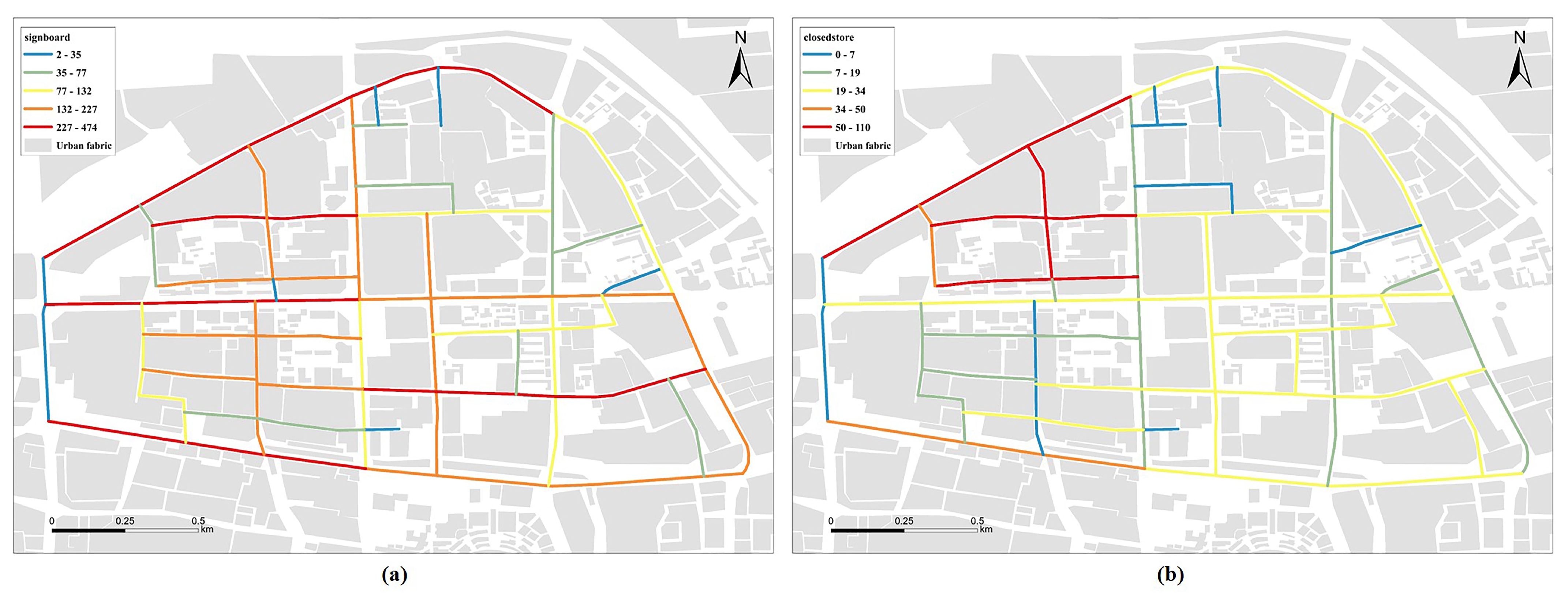
4.1.1. Economic Vitality of the Storefronts

As is illustrated in Figure 5, the distribution of economic vitality of the storefronts is presented from two perspectives. In terms of SD, which represents the overall performance of economic vitality, the highest value appears on five street segments: Jiahe Street, Fuguo Street, Huaihai West Road, Qingnian Road, and Jianguo West Road, from north to south. Interestingly, they are all basically east–west oriented, with the ranks ranging from primary to tertiary. At the same time, the other street segments with different performances of economic vitality are dispersed around the area. Both the location and the grade of the roads indicate that there is a relatively balanced distribution of economic vitality of storefronts in the old urban district, with relatively higher vitality in the western part.
From the perspective of CR, however, things seem to have changed. Higher values are denser in the western part compared to the eastern part, but differently from the connotation of the SD, they stand for higher probability of slow business, which can lead to the transfer or closure of shops. Meanwhile, there is a relatively general performance of the proxy in the eastern part. So, when we put the two kinds of performance of economic vitality together, it seems that there is an averaging mechanism in the whole area, with a phenomenon of higher CR accompanying higher SD. From this point of view, there is a lack of obvious advantageous agglomeration of storefronts.

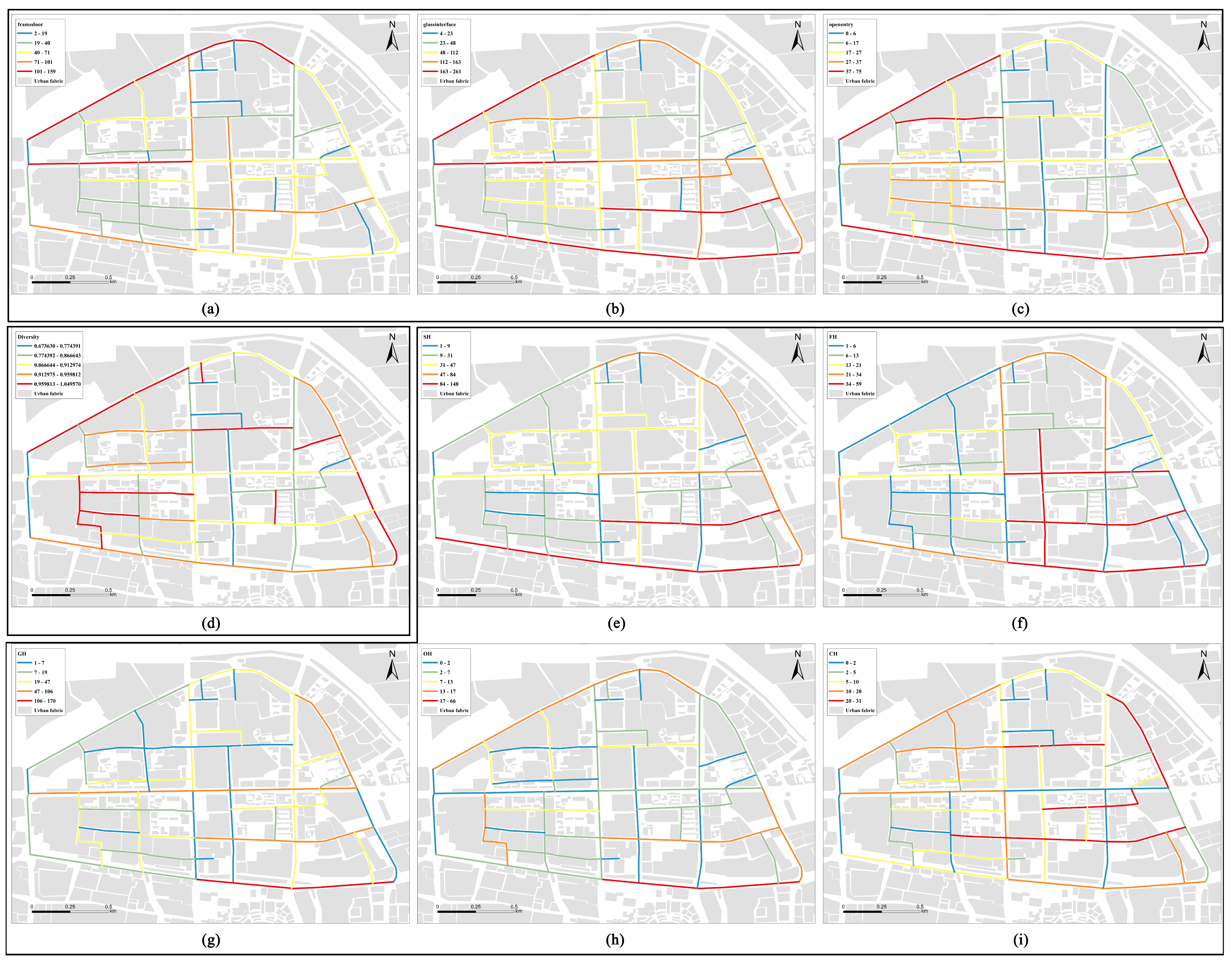
4.1.2. Characteristics of the Streetscape

According to the classification of the dependent variables, three aspects of the characteristics of the streetscape are presented in Figure 6: the elemental distribution of the interfaces, the diversity of the interfaces, and the spatial heterogeneity of the sections. The graphs corresponding to them are divided into three groups. The first one contains (a), (b), and (c); the second one has only (d); the last one includes (e) to (i).
First, as for the overall distribution of interfaces, the street segments with the highest values of FD are mainly concentrated in the northwestern part of the area, compared to the more balanced distribution of GI and OE, while the total number of OE is much less than that of FD and GI. Specifically, taking the intersection of the north–south-oriented Zhongshan Road and the west–east-oriented Huaihai Road as the original point of the four quadrants, there are lower values of FD and GI in the first and the third quadrants, while the first quadrant is at a low ebb for OE. This suggests that different types of interfaces seem to be influenced by different development strategies and react differently, with more intensified and diversified development located in the first quadrant and more traditional and small-scale roads in the third quadrant. At the same time, the five street segments with the highest values of SD have basically continued to perform well, exceeding the average level.
As for the diversity of the interfaces, differently from the above distribution, the area in the third quadrant has the most diversified performance; it may benefit from the more humanized spatial scale and easy atmosphere. The eastern part, as a comparison, has more fluctuation of the index, with more diversified interfaces around, which implies that most of the inner urban space looks monotonous. The phenomenon may be the expression of a kind of specialized business, but this is not the case. Actually, both intensified development of shopping centers and renovation projects of the historical area have emerged in the eastern part in recent years. Under this background, the risk of commercial homogenization is worthy of attention. Furthermore, we also noticed that the cross-shaped main roads as the axes have a relatively lower level of diversity. Considering the significant influence on the image of the area, the question of how to activate them deserves further research.
Spatial heterogeneity is revealed through the third group of illustrations in Figure 6. As a reflection of the sectional differences among the street segments, the heterogeneity is closely related to the asymmetric streetscape, which is far away from the traditional idea that a street is designed, managed, and developed as a symmetric spatial element. From the perspective of the distribution, among the graphs, the fourth quadrant has the highest level of heterogeneity, which indicates that there is an imbalanced commercial image and cityscape. In fact, the phenomenon is likely to result from dense green belts, undulation and adaptation of natural elements, large public institutions, and gated communities. To be specific, there is the lowest number of the maximum difference values for glassinterfaces and openentries, with limited high values scattered sporadically, as the graphs of GH and OH show. In terms of the performance regarding SH and FH, the highest values have accumulated gradually, from the southern Jianguo Road, spreading to the northern first quadrant. As for CH, higher values nearly appear in each quadrant, around the center of the old urban district. These results suggest that there is less difference in the street section for the glassinterfaces and the openentries, while the degree of heterogeneity increases from the signboards and the framedoors to the closedstores. From the perspective of numerical level, the peak intervals of the glassinterfaces and the signboards reach the highest values, compared to the other three types. This is consistent with the distribution of the signboards and the glassinterfaces, as shown in Figure 5a and Figure 6b.

4.2. Scale of Sampling Point: Correlation between Economic Vitality and the Streetscape

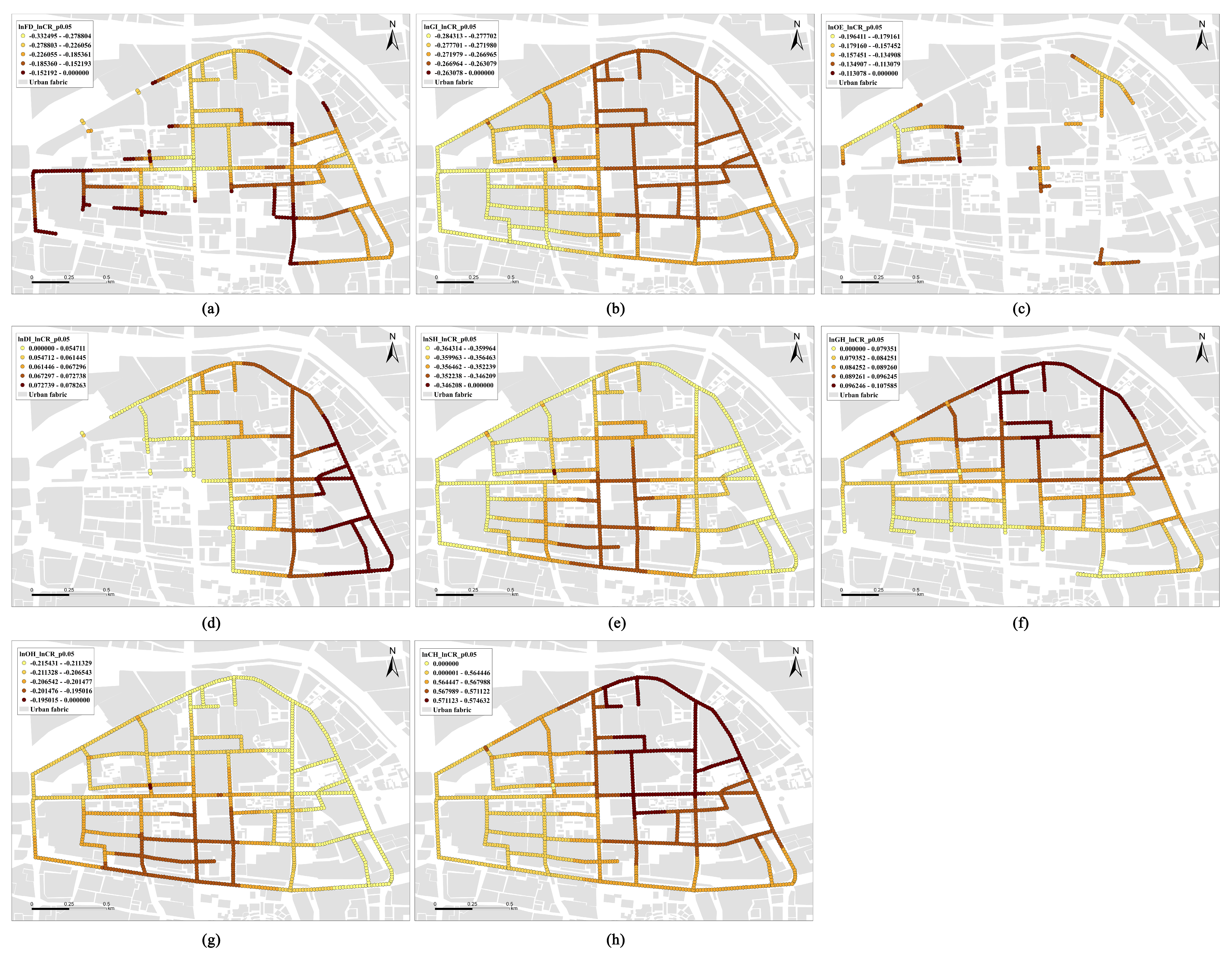
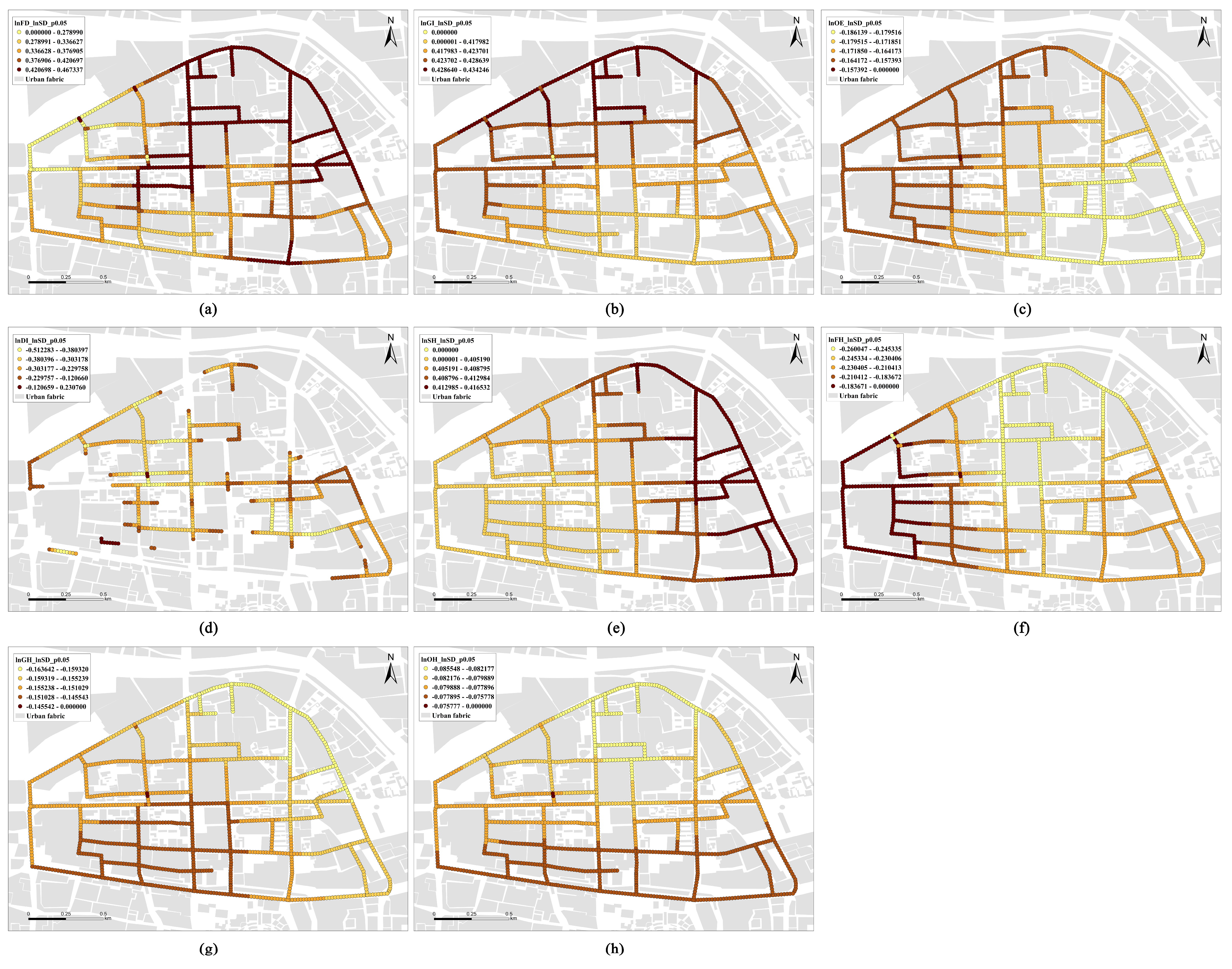
4.2.1. Results of the MGWR Model

Before the regression analysis, both the variance inflation factors (VIFs) of the variables and the spatial autocorrelation of the economic vitality need testing. First, the VIFs were calculated through the SPSS software to test the multicollinearity. As is shown in Table 5, all the VIF values of the independent variables are obviously less than 10 [44] or 7 [34], which means that there is no problem with the multicollinearity. Then, Moran’s I was used in the ArcGIS software to test the spatial autocorrelation of the dependent variables [44]. The results in Table 5 show that there are positive spatial autocorrelations for the indexes of economic vitality, with a p value of less than 0.01. Particularly, the degree of ln_SD is much stronger than that of ln_CR, indicating that different proxies for the same target are likely to display different degrees of spatial autocorrelation.
Taking ln_CR and ln_SD as the dependent variables, the performance of the MGWR model is different (see Table 6). For the corrected Akaike information criterion (AICc), the value of ln_SD is much lower than that of ln_CR; for the adjusted R-squared value, there is a higher performance of ln_SD as well. Therefore, the explanatory power of the model with ln_SD is better than that with ln_CR.

4.2.2. Correlation between Characteristics of the Streetscape and the Closedstore Rate

As the local parameter estimates in Table 6 show, there are three and three variables with totally positive and negative influences on ln_CR, respectively. The former groups consist of ln_CH, ln_GH, and ln_DI, while the latter contains ln_SH, ln_GI, and ln_OH, both in descending order of the absolute value. This suggests that lower difference values of the closedstores, glassinterfaces, and diversity index of interfaces, combined with higher difference value of signboards, sum of glassinterfaces, and difference value of openentries, can help reduce the rate of closure of storefronts. Meanwhile, the other variables of ln_FD, ln_OE, and ln_FH fluctuate between positive and negative values, indicating a varied influence on the dependent variable.
The parameters generated by MGWR are illustrated in full in Figure 7. Due to filtering the variables with a value of significance less than 0.05 (p < 0.05), the graph of FH was deleted because the number of sampling points that met the condition of the significance threshold was too small to express spatial meanings. The remaining eight graphs can be divided into three groups, according to the positive or negative effects on the rate of closedstores. The first group contains (d), (f), and (h), which all present positive correlation with ln_CR. Among them, the highest spatial heterogeneity brought by the glassinterfaces and the closedstores is found in the first quadrant, while the southeastern points form a heat core that is affected most by the diversity index of interfaces. Furthermore, all three graphs have a diffusion structure from a monocentric heat core to other areas.
The graphs (b), (e), and (g) show a global and significantly negative effect from every point and every street segment. The latter two have a similar structure, with the only heat core located in the south area, permeating into the surrounding roads and lanes, which implies reversely that the area has a relatively low rate of cloesedstores. At the same time, high values of the sum of glassinterfaces have occupied most of the eastern area, with a rather balanced but strong effect on the storefronts, Actually, the influences of the three factors are also quite steady, with their standard deviations ranging from 0.004 to 0.006.
As for the uncertain group containing (a) and (c) in Figure 6, the unstable distribution of the signboards and the openentries is clear, with scattered segments around the old urban district, especially for the latter. In addition, there are more heat points of the two variables, rather than a continuous heat area.

4.2.3. Correlation between Characteristics of the Streetscape and the Signboard Density

Table 6 lists three and four variables with totally positive and negative influences on ln_SD, respectively. The former refers to ln_FD, ln_GI, and ln_SH, with all local parameter estimates being over 0.2, while the latter consists of ln_FH, ln_OE, ln_GH, and ln_OH, in descending order of the absolute value of the mean. The results indicate that higher sums of framedoors and glassinterfaces, and difference value of the L- and R-sided signboards, together with lower difference values of framedoors, glassinterfaces, and openentries and the sum of openentries are beneficial to denser signboards of the storefronts, which represent a vital economy. The other two indexes, namely, ln_CH and ln_DI, have both positive and negative effects on the dependent variable. Particularly, the standard deviation of ln_DI reaches 0.143, which is the highest of the column.
As in the last session, the spatial distribution of the parameter estimates which were generated by MGWR and met the threshold requirement (p < 0.05) is illustrated in Figure 8. Similarly, the graph of CH was deleted, and we can interpret the remaining parameters in terms of three groups. The first one has significantly positive correlation with the density of the storefronts, containing (a), (b), and (e). Their positive influence is global in the district. Specifically, the latter two have similar diffusion structures, despite their heat areas being located in the north and east, respectively. The sum of the framedoors (ln_FD), however, permeates into other quadrants from the densest first quadrant, which has activated more of the inner area. In this way, the maximum of it exceeds the other two, reflecting a different but effective influence on the density of the signboards.
The four graphs labeled (c), (f), (g), and (h) in Figure 8 constitute the second group, which show significantly and globally negative effects on the dependent variable. They all have the spatial distribution of a monocentric heat area, offset to the west and south. Notably, however, the so-called heat area indicates low ebbs of the density of the signboards because of the negative influence. In other words, the yellow points, mainly located in the southeast, north, and northeast, stand for a better performance in terms of economic vitality.
As one component of the third group, the varied values and scattered distribution can be seen in the graph labeled (d). Although most of the points have negative values, a positive value can emerge at times, with a number as high as 0.231.

5. Discussion and Conclusions

Urban vitality has attracted much attention around the world, especially in areas with low vitality such as old urban districts. However, on the one hand, the proxies to reflect urban vitality mainly focus on the demand end, such as crowd agglomeration and people’s activities, while the supply end including other ordinary economic entities is relatively neglected. On the other hand, the utilization of SVIs deserves further exploration beyond traditional measurements based on the models and application scenarios adapted from autonomous driving such as sky, greenery, and so on. In addition, spatial heterogeneity, resulting from the sectional differences of the distribution of elements, has rarely received concern. All these issues have dominated research vision regarding urban vitality and restricted the potential spatial response from urban planners and designers. Therefore, based on machine learning technique and SVIs, we took the ordinary storefronts in the old urban district in Xuzhou, China, as the objects and developed an analytical framework from the scales of a street segment and a sampling point to depict the characteristics of the streetscape and economic vitality, respectively, and then reveal their correlation. Notably, the vitality was presented from two perspectives as well, including both the alive and the closed stores. Our findings comprise three aspects: (1) although the sum of the storefronts is more often used, combining the alive and the closed businesses is beneficial to reflecting the economic vitality in an eclectic and real way; (2) as a reflection of the spatial heterogeneity and sectional differences of elements, the asymmetric streetscape has a significant influence on the economic vitality; and (3) although different factors from the streetscape can influence economic vitality differently, based on varied proxies of the vitality, three factors, namely, higher SH, higher GI, and lower GH, can benefit the economic vitality.
The development of tools is closely related to their application. Although SVIs and machine learning algorithms have been used in more and more studies recently, most of them limit the application scenarios only to calculate indexes such as the proportion of greenery, sky, pavement, building façade, traffic, etc. [35,36,59,60]. In this paper, we identified more customized spatial information and excavated the socio-economic features behind the images. On the one hand, more commercial elements of the streetscape were chosen and analyzed in this paper, in contrast to the prior explorations that paid more attention to the identification and classification of different signage, logos, and trademarks of businesses [39,40]. In terms of the common types of labels, three possible explanations for the higher AP value of the signboards with fewer photos for training in our model are more attention to the general features rather than the specific brands, more accurate boundaries with polygon annotations, and the iteration of newer version of the algorithm. On the other hand, compared to other vitality-related studies, our approaches explore a multiscale application, not just the scales of a street segment and a sampling point used in this paper. In fact, it can be integrated into a macro-scale analysis in a land grid created by the fishnet tool in ArcGIS, and smooth transition between the different scales can be achieved with different spatial intervals between the points of the minimum scale.
As one of the most important premises, deciding what kinds of proxies to use to represent economic vitality has a significant influence on the later analysis. In the literature review, we have found that many researchers adopt POI data from Dianping, Gaode Map, Baidu Map, etc., and take the sum of the businesses or the density in an area as the index of economic vitality [5,27,32,33,42,45,46,47,48,49]. Consistent with this approach, we use the storefront density (SD) as a proxy. Given that the real status of the storefronts is changing due to commercial competition, however, the closedstore rate (CR) is taken as another proxy in this paper as a complement from the opposite perspective. Meanwhile, the better performance of the machine learning algorithm for the signboards and the closedstores is beneficial to depicting the indexes as well. Taking them together for analysis, we noticed that a higher CR value is accompanied by a higher SD value in the street segments of the whole area, showing an averaging mechanism of the economic vitality, which verifies our opinion that only using the sum of the shops such as with SD is insufficiently persuasive to represent economic vitality.
The idea of comparing the sectional differences of the indexes to reveal the spatial heterogeneity of the sampling points is one of the contributions of our paper. To the best of our knowledge, the approach has never been systematically put forward for fine-grained spatial analysis in prior studies, except when Ye et al. used the method only to acquire the SVIs [40]. This is partly because of the emphasis on the traffic function for the higher-level roads and the traditional hypothesis of the symmetric commercial streetscape for the lower-level roads. In addition, the method of development and transfer of the basic land units like parcels is likely to result in heterogeneity. Given that the asymmetric streetscape has certain effects on the continuity, density, and atmosphere of commercial businesses, and on consumers’ perception and movement, this phenomenon deserves further exploration, especially for those areas with more single-sided distributions of storefronts.
In terms of the results of the correlation analysis, taking higher positive values of the independent variables for ln_SD and lower negative values of them for ln_CR as the aim, we find that both higher ln_SH and higher ln_GI are beneficial to vibrant storefronts, while higher ln_GH is bad for the economic vitality. Some of the findings are in accord with traditional studies indicating that more glass interfaces have a positive effect on the perception of street space [61], which perhaps provides new insights into asymmetric commercial streetscapes and the operation of the storefronts.
For urban planners, designers and decision-makers, our research is likely to support their work in at least two aspects. First, it can help refined and efficient urban physical examination and targeted governance. In recent years, urban physical examination has been launched as a pilot project in more and more Chinese cities, with the interval in some cities being as short as one year, not to mention the higher frequency of smaller areas. With our approach in this paper, street segments and points with low economic vitality and the related characteristics of the streetscape can be seen in a sensible, efficient, and locatable way, which enables more accurate intervention by official powers. Second, as decay clues in old urban districts can be perceived more or less through SVIs, our study gives an instance of their detection in such areas. Particularly, it can display both the characteristics of the streetscape and the economic vitality behind the images, with better performance when combined with other statistics and big data.
Despite more perspectives, dual spatial scales, and extended exploration of sectional differences of elements, admittedly, there are some limitations to this study as well. First, although we attempt to focus on economic entities directly by using SVIs, other public institutions also appear in the images and are identified by our machine learning model, which can increase or decrease the density of the commercial elements. Second, the SVIs collected in our study are mainly from 2018, with some of them having been renewed in recent years. Actually, considering the cost and the potential profit, similar problems exist in other map platforms as well. However, because the outbreak of COVID-19 and the establishment of lockdown policies for a relatively long time in China have slowed down economic transactions and nearly all the other projects, the difference between the real situation and the SVIs is limited. Third, as we have pointed out in the aforementioned content, using the deep excavation of SVIs to focus on the supply end is the main target in the paper. However, the performances of the machine learning model on the five kinds of elements are not equal, with higher AP values on the relatively evident and shallow features of the images, which can affect the accurate description of all the variables.
In future studies about economic vitality of storefronts and related proxies, we recommend that different perspectives and entities of the vitality, as well as the phenomenon of asymmetry created by the processes of design, management, and adaptive reutilization, be given more attention. In addition, we also suggest that future research extend the scope in a diachronic analysis and focus on the daily change in interactions with consumers, combined with deeper exploration of the potential of image perception and identification.

Author Contributions

Conceptualization, Keran Li; methodology, Keran Li; software, Keran Li; validation, Keran Li; formal analysis, Keran Li; investigation, Keran Li; resources, Keran Li and Yan Lin; data curation, Keran Li; writing—original draft preparation, Keran Li; writing—review and editing, Keran Li and Yan Lin; visualization, Keran Li; supervision, Yan Lin; project administration, Keran Li and Yan Lin; funding acquisition, Yan Lin. All authors have read and agreed to the published version of the manuscript.

Funding

This research was funded by the “Project of Social Science Foundation of Jiangsu Province, 20YSC010”.

Data Availability Statement

The data presented in this study are unavailable due to privacy restrictions.

Conflicts of Interest

The authors declare no conflict of interest.

References

  1. Lashgari, Y.S.; Shahab, S. The Impact of the COVID-19 Pandemic on Retail in City Centres. Sustainability 2022, 14, 11463. [Google Scholar] [CrossRef]
  2. Valdenebro, J.-V.; Gimena, F.N. Urban utility tunnels as a long-term solution for the sustainable revitalization of historic centres: The case study of Pamplona-Spain. Tunn. Undergr. Space Technol. 2018, 81, 228–236. [Google Scholar] [CrossRef]
  3. Günaydın, A.S.; Altunkasa, M.F. Developing the socio-spatial integration of historical city centers with spatial strategies: The case of Gaziantep. Environ. Dev. Sustain. 2022, 24, 8092–8114. [Google Scholar] [CrossRef]
  4. Rogerson, R.J.; Giddings, B. The future of the city centre: Urbanisation, transformation and resilience—A tale of two Newcastle cities. Urban Stud. 2021, 58, 1967–1982. [Google Scholar] [CrossRef]
  5. Xia, C.; Zhang, A.; Yeh, A.G.O. The Varying Relationships between Multidimensional Urban Form and Urban Vitality in Chinese Megacities: Insights from a Comparative Analysis. Ann. Am. Assoc. Geogr. 2022, 112, 141–166. [Google Scholar] [CrossRef]
  6. Nadalin, V.; Igliori, D. Empty spaces in the crowd. Residential vacancy in São Paulo’s city centre. Urban Stud. 2017, 54, 3085–3100. [Google Scholar] [CrossRef]
  7. Larraz, B.; García-Gómez, E. Depopulation of Toledo’s historical centre in Spain? Challenge for local politics in world heritage cities. Cities 2020, 105, 102841. [Google Scholar] [CrossRef]
  8. Liu, Z.; Wang, S.; Wang, F. Isolated or integrated? Planning and management of urban renewal for historic areas in Old Beijing city, based on the association network system. Habitat Int. 2019, 93, 102049. [Google Scholar] [CrossRef]
  9. United Nations. Partnership for Sustainable Development Goals: A Legacy Review towards Realizing the 2030 Agenda. Available online: https://sustainabledevelopment.un.org/sdinaction/publication/partnerships-a-legacy-review (accessed on 8 May 2023).
  10. Zhang, H.; Cong, C.; Chakraborty, A. Exploring the institutional dilemma and governance transformation in China’s urban regeneration: Based on the case of Shanghai Old Town. Cities 2022, 131, 103915. [Google Scholar] [CrossRef]
  11. Ryberg, S.R. Historic Preservation’s Urban Renewal Roots: Preservation and Planning in Midcentury Philadelphia. J. Urban Hist. 2013, 39, 193–213. [Google Scholar] [CrossRef]
  12. Zhao, Y.; Ponzini, D.; Zhang, R. The policy networks of heritage-led development in Chinese historic cities: The case of Xi’an’s Big Wild Goose Pagoda area. Habitat Int. 2020, 96, 102106. [Google Scholar] [CrossRef]
  13. Alexander, A.; Teller, C.; Wood, S. Augmenting the urban place brand—On the relationship between markets and town and city centres. J. Bus. Res. 2020, 116, 642–654. [Google Scholar] [CrossRef]
  14. Slach, O.; Nováček, A.; Bosák, V.; Krtička, L. Mega-retail-led regeneration in the shrinking city: Panacea or placebo? Cities 2020, 104, 102799. [Google Scholar] [CrossRef]
  15. Hangebruch, N.; Othengrafen, F. Resilient Inner Cities: Conditions and Examples for the Transformation of Former Department Stores in Germany. Sustainability 2022, 14, 8303. [Google Scholar] [CrossRef]
  16. Guimarães, P.P.C. An evaluation of urban regeneration: The effectiveness of a retail-led project in Lisbon. Urban Res. Pract. 2017, 10, 350–366. [Google Scholar] [CrossRef]
  17. Xie, S.; Zhang, X.; Li, Y.; Skitmore, M. Echoes of Italian lessons on the typo-morphological approach: A planning proposal for Gulangyu Island, China. Habitat Int. 2017, 69, 1–17. [Google Scholar] [CrossRef] [Green Version]
  18. Zhu, H.; Liu, J.; Liu, H.; Wang, X.; Ma, Y. Recreational Business District boundary identifying and spatial structure influence in historic area development: A case study of Qianmen area, China. Habitat Int. 2017, 63, 11–20. [Google Scholar] [CrossRef]
  19. Zou, H.; Liu, R.; Cheng, W.; Lei, J.; Ge, J. The Association between Street Built Environment and Street Vitality Based on Quantitative Analysis in Historic Areas: A Case Study of Wuhan, China. Sustainability 2023, 15, 1732. [Google Scholar] [CrossRef]
  20. Jacobs, J. The Death and Life of Great American Cities; Vintage Book Company: New York, NY, USA, 1961. [Google Scholar]
  21. Gehl, J. Life between Buildings; Danish Architectural Press: Copenhagen, Denmark, 1971. [Google Scholar]
  22. Lynch, K. Good City Form; MIT Press: Cambridge, MA, USA, 1981. [Google Scholar]
  23. Whyte, W.H. The Social Life of Small Urban Spaces; The Conservation Foundation: Washington, DC, USA, 1980. [Google Scholar]
  24. Maas, P.R. Towards a Theory of Urban Vitality. Doctor’s Thesis, University of British Columbia, Vancouver, BC, Canada, 1984. [Google Scholar]
  25. Montgomery, J. Making a city: Urban vitality, vitality and urban design. J. Urban Des. 1998, 3, 93–116. [Google Scholar] [CrossRef]
  26. Katz, P.; Scully, V.J.; Bressi, T.W. The New Urbanism: Toward an Architecture of Community; McGraw-Hill: New York, NY, USA, 1994. [Google Scholar]
  27. Xia, C.; Yeh, A.G.O.; Zhang, A. Analyzing spatial relationships between urban land use intensity and urban vitality at street block level: A case study of five Chinese megacities. Landsc. Urban Plan. 2020, 193, 103669. [Google Scholar] [CrossRef]
  28. Li, M.; Pan, J. Assessment of Influence Mechanisms of Built Environment on Street Vitality Using Multisource Spatial Data: A Case Study in Qingdao, China. Sustainability 2023, 15, 1518. [Google Scholar] [CrossRef]
  29. Li, Y.; Yabuki, N.; Fukuda, T. Exploring the association between street built environment and street vitality using deep learning methods. Sust. Cities Soc. 2022, 79, 103656. [Google Scholar] [CrossRef]
  30. Wu, W.; Niu, X.; Li, M. Influence of Built Environment on Street Vitality: A Case Study of West Nanjing Road in Shanghai Based on Mobile Location Data. Sustainability 2021, 13, 1840. [Google Scholar] [CrossRef]
  31. Chen, W.; Wu, A.N.; Biljecki, F. Classification of urban morphology with deep learning: Application on urban vitality. Comput. Environ. Urban Syst. 2021, 90, 101706. [Google Scholar] [CrossRef]
  32. Wu, J.; Lu, Y.; Gao, H.; Wang, M. Cultivating historical heritage area vitality using urban morphology approach based on big data and machine learning. Comput. Environ. Urban Syst. 2022, 91, 101716. [Google Scholar] [CrossRef]
  33. Ye, Y.; Li, D.; Liu, X. How block density and typology affect urban vitality: An exploratory analysis in Shenzhen, China. Urban Geogr. 2018, 39, 631–652. [Google Scholar] [CrossRef]
  34. Long, Y.; Huang, C. Does block size matter? The impact of urban design on economic vitality for Chinese cities. Environ. Plan. B-Urban Anal. City Sci. 2019, 46, 406–422. [Google Scholar] [CrossRef] [Green Version]
  35. Jiang, Y.; Han, Y.; Liu, M.; Ye, Y. Street vitality and built environment features: A data-informed approach from fourteen Chinese cities. Sust. Cities Soc. 2022, 79, 103724. [Google Scholar] [CrossRef]
  36. Li, X.; Li, Y.; Jia, T.; Zhou, L.; Hijazi, I.H. The six dimensions of built environment on urban vitality: Fusion evidence from multi-source data. Cities 2022, 121, 103482. [Google Scholar] [CrossRef]
  37. Wu, J.; Ta, N.; Song, Y.; Lin, J.; Chai, Y. Urban form breeds neighborhood vibrancy: A case study using a GPS-based activity survey in suburban Beijing. Cities 2018, 74, 100–108. [Google Scholar] [CrossRef]
  38. Wu, W.; Ma, Z.; Guo, J.; Niu, X.; Zhao, K. Evaluating the Effects of Built Environment on Street Vitality at the City Level: An Empirical Research Based on Spatial Panel Durbin Model. Int. J. Environ. Res. Public Health 2022, 19, 1664. [Google Scholar] [CrossRef]
  39. Tsai, T.-H.; Cheng, W.-H.; You, C.-W.; Hu, M.-C.; Tsui, A.W.; Chi, H.-Y. Learning and Recognition of On-Premise Signs from Weakly Labeled Street View Images. IEEE Trans. Image Process. 2014, 23, 1047–1059. [Google Scholar] [CrossRef] [PubMed]
  40. Ye, N.; Wang, B.; Kita, M.; Xie, M.; Cai, W. Urban Commerce Distribution Analysis Based on Street View and Deep Learning. IEEE Access 2019, 7, 162841–162849. [Google Scholar] [CrossRef]
  41. Zamir, A.R.; Darino, A.; Patrick, R.; Shah, M. Street View Challenge: Identification of Commercial Entities in Street View Imagery. In Proceedings of the IEEE 2021 Tenth International Conference on Machine Learning and Applications (ICMLA 2011), Honolulu, HI, USA, 18–21 December 2011. [Google Scholar] [CrossRef]
  42. Li, Q.; Cui, C.; Liu, F.; Wu, Q.; Run, Y.; Han, Z. Multidimensional Urban Vitality on Streets: Spatial Patterns and Influence Factor Identification Using Multisource Urban Data. ISPRS Int. J. Geo-Inf. 2022, 11, 2. [Google Scholar] [CrossRef]
  43. Li, M.; Liu, J.; Lin, Y.; Xiao, L.; Zhou, J. Revitalizing historic districts: Identifying built environment predictors for street vibrancy based on urban sensor data. Cities 2021, 117, 103305. [Google Scholar] [CrossRef]
  44. Chen, Y.; Yu, B.; Shu, B.; Yang, L.; Wang, R. Exploring the spatiotemporal patterns and correlates of urban vitality: Temporal and spatial heterogeneity. Sust. Cities Soc. 2023, 91, 104440. [Google Scholar] [CrossRef]
  45. Zhang, A.; Li, W.; Wu, J.; Lin, J.; Chu, J.; Xia, C. How can the urban landscape affect urban vitality at the street block level? A case study of 15 metropolises in China. Environ. Plan. B-Urban Anal. City Sci. 2021, 48, 1245–1262. [Google Scholar] [CrossRef]
  46. Zikirya, B.; He, X.; Li, M.; Zhou, C. Urban Food Takeaway Vitality: A New Technique to Assess Urban Vitality. Int. J. Environ. Res. Public Health 2021, 18, 3578. [Google Scholar] [CrossRef]
  47. Porta, S.; Strano, E.; Iacoviello, V.; Messora, R.; Latora, V.; Cardillo, A.; Wang, F.; Scellato, S. Street Centrality and Densities of Retail and Services in Bologna, Italy. Environ. Plan. B-Plan. Des. 2009, 36, 450–465. [Google Scholar] [CrossRef] [Green Version]
  48. Lin, G.; Chen, X.; Liang, Y. The location of retail stores and street centrality in Guangzhou, China. Appl. Geogr. 2018, 100, 12–20. [Google Scholar] [CrossRef]
  49. Kim, S.; Woo, A. Streetscape and business survival: Examining the impact of walkable environments on the survival of restaurant businesses in commercial areas based on street view images. J. Transp. Geogr. 2022, 105, 103480. [Google Scholar] [CrossRef]
  50. Carmelino, G.; Hanazato, T. The built environment of Japanese shopping streets as visual information on pedestrian vibrancy. Front. Archit. Res. 2019, 8, 261–273. [Google Scholar] [CrossRef]
  51. Zhao, M.; Zhou, Y.; Li, X.; Cheng, W.; Zhou, C.; Ma, T.; Li, M.; Huang, K. Mapping urban dynamics (1992–2018) in Southeast Asia using consistent nighttime light data from DMSP and VIIRS. Remote Sens. Environ. 2020, 248, 111980. [Google Scholar] [CrossRef]
  52. Redmon, J.; Divvala, S.; Girshick, R.; Farhadi, A. You Only Look Once: Unified, Real-Time Object Detection. In Proceedings of the 2016 IEEE Conference on Computer Vision and Pattern Recognition (CVPR), Las Vegas, NV, USA, 27–30 June 2016. [Google Scholar] [CrossRef] [Green Version]
  53. Palmer, G.; Green, M.; Boyland, E.; Vasconcelos, Y.S.R.; Savani, R.; Singleton, A. A deep learning approach to identify unhealthy advertisements in street view images. Sci. Rep. 2021, 11, 4884. [Google Scholar] [CrossRef]
  54. Suel, E.; Polak, J.W.; Bennett, J.E.; Ezzati, M. Measuring social, environmental and health inequalities using deep learning and street imagery. Sci. Rep. 2019, 9, 6229. [Google Scholar] [CrossRef] [Green Version]
  55. Lin, Y.; Luo, P. A Study on the Implicit Structure of Historical Environment in Urban Space of Xuzhou. Sustainability 2022, 14, 6837. [Google Scholar] [CrossRef]
  56. Xuzhou Municipal People’s Government. Master Plan for the Territorial Space of Xuzhou (2021–2035). Available online: http://www.xz.gov.cn/001/001007/20230315/93f79f05-c3e3-4ce4-923a-a4a71c28aaa3.html (accessed on 10 May 2023).
  57. Fotheringham, A.S.; Yang, W.; Kang, W. Multiscale Geographically Weighted Regression (MGWR). Ann. Am. Assoc. Geogr. 2017, 107, 1247–1265. [Google Scholar] [CrossRef]
  58. Shannon, C. A mathematical theory of communication. Bell Syst. Tech. J. 1948, 27, 379–423, 623–656. [Google Scholar] [CrossRef] [Green Version]
  59. Li, X.; Zhang, C.; Li, W.; Richard, R.; Meng, Q.; Zhang, W. Assessing street-level urban greenery using Google Street View and a modified green view index. Urban For. Urban Green. 2015, 14, 675–685. [Google Scholar] [CrossRef]
  60. Ma, X.; Ma, C.; Wu, C.; Xi, Y.; Yang, R.; Peng, N.; Zhang, C.; Ren, F. Measuring human perceptions of streetscapes to better inform urban renewal: A perspective of scene semantic parsing. Cities 2021, 110, 103086. [Google Scholar] [CrossRef]
  61. Du, Y.; Huang, W. Evaluation of Street Space Quality Using Streetscape Data: Perspective from Recreational Physical Activity of the Elderly. ISPRS Int. J. Geo-Inf. 2022, 11, 241. [Google Scholar] [CrossRef]
Figure 1. Study area.
Ijgi 12 00267 g001
Figure 2. The evolution of the study area in the recent century. Note: both the left street map from the Annals of Tongshan County published in 1904 and the right satellite map based on Google Maps are adapted by the authors.
Ijgi 12 00267 g002
Figure 3. Analysis Framework.
Ijgi 12 00267 g003
Figure 4. Performance of the training model with confusion matrix and P–R curve.
Ijgi 12 00267 g004
Figure 5. Economic vitality of the storefronts: (a) from the perspective of SD; and (b) from the perspective of CR.
Ijgi 12 00267 g005
Figure 6. Characteristics of the streetscape: (a) FD; (b) GI; (c) OE; (d) DI; (e) SH; (f) FH; (g) GH; (h) OH; and (i) CH. Note: the graphs are arranged into three groups with black borderlines around them.
Ijgi 12 00267 g006
Figure 7. Effects on CR: (a) FD; (b) GI; (c) OE; (d) DI; (e) SH; (f) GH; (g) OH; and (h) CH. Note: the graph of FH is not shown here due to the very limited number of points with p < 0.05.
Ijgi 12 00267 g007
Figure 8. Effects on SD: (a) FD; (b) GI; (c) OE; (d) DI; (e) SH; (f) FH; (g) GH; and (h) OH. Note: the graph of CH is not shown here due to the very limited number of points with p < 0.05.
Ijgi 12 00267 g008
Table 1. Related literature on economic vitality and the measurement of businesses.
LiteratureStudy AreaScaleProxyData Source
Long, & Huang, 2019 [34]286 largest Chinese citiesLand grids of 1 km by 1 kmSocial media comments, sign-ins; housing price dataDianping; Sina Weibo; Soufun
Ye, Li, & Liu, 2018 [33]Shenzhen, ChinaStreet blockSmall catering businessDianping
Li et al., 2022 [42]Chengdu, ChinaStreet segmentUser word-of-mouth weightsDianping
Zikirya et al., 2021 [46]Beijing, Shanghai, Guangzhou, ChinaLand grids with different scalesTake-away dataMeituan
Wu et al., 2022 [32]12 Chinese citiesBlockGeo-tagged small food facilities; night-time light dataPOI data from Baidu Map
Zhang et al., 2021 [45]15 Chinese metropolisesStreet blockSmall catering business; night-time light dataDianping; VIIRS DNB
Xia, Yeh, & Zhang, 2020 [27]5 Chinese megacitiesStreet blockSmall catering business; night-time light dataDianping; VIIRS DNB
Xia, Zhang, & Yeh, 2021 [5]15 Chinese megacitiesStreet blockRestaurant data; nighttime light dataDianping; VIIRS DNB
Porta et al., 2009 [47]Bologna, ItalyStreet segmentRetail and service entitiesMunicipality of Bologna
Lin, Chen, & Liang, 2018 [48]Guangzhou, ChinaStreet segmentRetail storesPOI data from Baidu Map
Kim, & Woo, 2022 [49]Seoul, KoreaCommercial areaRestaurant businessesKorean local data
Table 2. Five kinds of components in the streetscape data.
ClassificationCase PhotoDefinition
SignboardIjgi 12 00267 i001(1) The number of storefronts, whether in business or not. (2) A representative of economic vitality.
FramedoorIjgi 12 00267 i002(1) Entrances with clear frames around them. (2) A kind of interface of the storefronts which mainly operate indoors.
GlassinterfaceIjgi 12 00267 i003(1) Glass occupying the main part of the holes of gateways/windows, with no frames around. (2) A kind of interface of the storefronts which need to be displayed externally.
OpenentryIjgi 12 00267 i004(1) Only edges can be seen, with shadows or different kinds of goods in them. (2) A kind of interface of the storefronts which require direct and constant outdoor relationships.
ClosedstoreIjgi 12 00267 i005(1) Storefronts that are not in business. (2) Another representative of economic vitality from the opposite perspective.
Table 3. The training environment and settings of some hyperparameters.
IndexValue/Model
CPUAMD Ryzen 7 5800H with Radeon Graphics 3.20 GHz
GPUNVIDIA GeForce RTX 3070
batch-size8
epochs300
img640
lrf0.01
momentum0.937
weight decay0.0005
Table 4. Variables, the description and calculation methods.
VariablesAbbr.UnitDescriptionCalculation Methods
Dependent variables
storefront densitySD/(100 m)The ratio of the sum of the signboards to the length of the unit S D i = S F l i + S F r i l i
where SFli and SFri are the sums of the signboards of the i-th unit from the L- and R-side, respectively, and li is the length of the range of the i-th unit.
closedstore rateCR%The ratio of the sum of the closedstores to the sum of the signboards C R i = C S l i + C S r i S F l i + S F r i
where CSli and CSri are the sums of the closedstores of the i-th unit from the L- and R-side, respectively.
Independent variables
interface preferenceFD-The sum of the framedoors of the unit F D i = F D l i + F D r i
where FDli and FDri are the sums of the framedoors of the i-th unit from the L- and R-side, respectively.
GI-The sum of the glassinterfaces of the unit G I i = G I l i + G I r i
where GIli and GIri are the sums of the glassinterfaces of the i-th unit from the L- and R-side, respectively.
OE-The sum of the openentries of the unit O E i = O E l i + O E r i
where OEli and OEri are the sums of the openentries of the i-th unit from the L- and R-side, respectively.
diversity indexDI-The degree of diversity of the interface calculated by Shannon entropy D I i = ( P j   *   ln P j )
where Pj is the proportion of the j-th type of the interface, i.e., PFD, PGI, and POE within the i-th unit.
elemental heterogeneitySH-The difference value between the signboards of L- and R-side of the unit S H i = S F l i S F r i
FH-The difference value between the framedoors of L- and R-side of the unit F H i = F D l i F D r i
GH-The difference value between the glassinterfaces of L- and R-side of the unit G H i = G I l i G I r i
OH-The difference value between the openentries of L- and R-side of the unit O H i = O E l i O E r i
CH-The difference value between the closedstores of L- and R-side of the unit C H i = C S l i C S r i
Table 5. Results of the multicollinearity and the spatial autocorrelation tests.
VariableValueVariableValue
Multicollinearity test
ln_FD2.119ln_GI2.191
ln_OE1.494ln_SH2.118
ln_FH2.981ln_GH2.942
ln_OH2.819ln_CH2.544
ln_DI1.138
Autocorrelation test
ln_CRMoran’s I 0.265ln_SDMoran’s I 0.768
z score 5.165 z score 14.925
p < 0.01 p < 0.01
Table 6. Performance of the MGWR model and the results of the statistics.
Variablesln_CRln_SD
MeanStd. DeviationMinMaxMeanStd. DeviationMinMax
Intercept−0.0060.278−0.6370.6500.0170.110−0.2420.318
ln_FD−0.1520.088−0.3320.0980.3840.0600.2140.467
ln_GI−0.2700.006−0.284−0.2630.4230.0060.4120.434
ln_OE−0.0600.065−0.1960.099−0.1700.009−0.186−0.157
ln_SH−0.3570.004−0.364−0.3460.4080.0050.4020.417
ln_FH−0.0010.009−0.0170.019−0.2210.028−0.260−0.163
ln_GH0.0860.0080.0740.108−0.1540.004−0.164−0.146
ln_OH−0.2070.005−0.215−0.195−0.0790.002−0.086−0.076
ln_CH0.5680.0040.5600.5750.0100.006−0.0030.020
ln_DI0.0540.0150.0260.078−0.1780.143−0.5120.231
Log-likelihood−1320.349−821.205
AIC2852.1461864.579
AICc2871.8851886.463
R20.5160.782
Adj. R20.4720.761
Disclaimer/Publisher’s Note: The statements, opinions and data contained in all publications are solely those of the individual author(s) and contributor(s) and not of MDPI and/or the editor(s). MDPI and/or the editor(s) disclaim responsibility for any injury to people or property resulting from any ideas, methods, instructions or products referred to in the content.

