Energy-Efficient 3D Path Planning for Complex Field Scenes Using the Digital Model with Landcover and Terrain

Abstract

Path planning is widely used in many domains, and it is crucial for the advancement of map navigation, autonomous driving, and robot path planning. However, existing path planning methods have certain limitations for complex field scenes with undulating terrain and diverse landcover types. This paper presents an energy-efficient 3D path planning algorithm based on an improved A* algorithm and the particle swarm algorithm in complex field scenes. The evaluation function of the A* algorithm was improved to be suitable for complex field scenes. The slope parameter and friction coefficient were respectively used in the evaluation function to represent different terrain features and landcover types. The selection of expanding nodes in the algorithm depends not only on the minimum distance but also on the minimum consumption cost. Furthermore, the turning radius factor and slope threshold factor of vehicles were added to the definition of impassable points in the improved A* algorithm, so that the accessibility of path planning could be guaranteed by excluding some bends and steep slopes. To meet the requirements for multi-target path planning, the improved A* algorithm was used as the fitness function of the particle swarm algorithm to solve the traveling salesman problem. The experimental results showed that the proposed algorithm is capable of multi-target path planning in complex field scenes. Furthermore, the path planned by this algorithm is more passable and more energy efficient. In this experimental environment model, the average energy-saving efficiency of the path planned by the improved algorithm is 14.7% compared to the traditional A* algorithm. This would be beneficial to the development of ecotourism and geological exploration.

1. Introduction

With the increasing demand for driving in wilderness environments (ecotourism and geological exploration), the study of 3D path planning in complex field scenes with undulating terrain and diverse landcover types is becoming more and more popular. Path planning is not only one of the core elements of map navigation but also the main research content in autonomous driving, UAV navigation, and robot navigation. Traditional path planning algorithms are mostly used in urban areas, so most of them are not suitable for complex field scenes with undulating terrain and diverse landcover types. Due to the limited energy supply in wilderness environments, energy consumption should be taken into account as one of the most important factors. Therefore, it is necessary to study energy-efficient 3D path planning for complex field scenes.

The commonly used path planning algorithms for vehicles could be divided into two types. One is traditional algorithms, such as artificial potential field method [1,2], rapidly exploring random tree (RRT) [3,4,5], and A* algorithm [6,7,8]; and the other is intelligent algorithms, such as genetic algorithm (GA) [9,10,11], ant colony optimization (ACO) [12,13], particle swarm optimization (PSO) [14,15,16], and neural network algorithm [17,18]. This study is about global path planning based on an environment model with known terrain and landcover. Among the above algorithms, intelligent algorithms, RRT and A* algorithm, were often used in global path planning [19,20]. Intelligent algorithms have the advantages of simple calculation, strong robustness, and flexible application in various tasks [21,22,23,24]. However, they also have some disadvantages in solving the problem of high-dimension path planning, including slow convergence speed, low convergence accuracy, and incidental local optimal solution [21,22,25,26,27]. Therefore, intelligent algorithms have certain limitations when applied to large-scale complex environments. The RRT method is a sampling-based path planning technique for solving complex constraint problems and has the benefit of great search efficiency [3,28]. However, the quality of the planned path is average, and the applicable environment is limited (not suitable for narrow and long spaces) [29,30]. Furthermore, the RRT results have strong randomness, which makes it difficult to apply to complex field environments with harsh traffic conditions. The A* algorithm is an efficient heuristic search algorithm based on graph traversal, which has the advantages of rapid response to the environment, high accuracy, and good stability [7]. However, as the number of nodes increases, the search efficiency will decrease. In the research background of this paper, the accuracy of path planning results has a significant impact on energy consumption, and accuracy deserves greater consideration than time cost. Thus, the A* algorithm was selected and improved for path planning in this study.

Up until now, some studies have been conducted to improve the A* algorithm, such as [31], by setting the filter function to solve the problem of excessively large turning angles and irregular paths. However, it is still limited to flat path planning without taking slope into account. A guidance-based A* algorithm is proposed to improve obstacle avoidance performance by improving the heuristic function [32]. However, the influence of vehicle characteristics was not considered in the algorithm. A method that is more conducive to motion control and smoother path planning is proposed in the literature [33]. However, the energy consumption caused by smoothing the path is not considered. In this study, the A* algorithm is improved to realize energy-saving path planning in complex field scenes. The evaluation function of the A* algorithm would be improved by adding terrain and landcover factors to evaluation criteria of extension nodes, with the constraint of maximum slope and turning radius depending on the movement characteristics of vehicles.

In actual application scenarios, path planning is commonly used among multiple targets and not only between two targets. The Traveling Salesman Problem (TSP) is a classical combinatorial optimization problem in the multi-target path planning. A manifold of swarm intelligence (SI) algorithms, such as ACO, PSO, and bee colony optimization (BCO) and their variants, have been used to solve TSP successfully [34,35,36]. PSO is based on social interactions between entities and was first inspired by bird flocks. Compared with other SI algorithms, PSO has the advantages of a simpler structure, fewer parameters, and faster search speed [37]. Thus, PSO would be used to solve the TSP in this study.

In view of the current problems, such as the travel modes of different kinds of vehicles, differences in terrain and landcover, and the optimal order of multiple targets, this paper studied the multi-target 3D path planning problem in complex field scenes. We took an area in Changning County, Yunnan Province, China, as an example in this study. Changning County is a mountainous area with abundant landcover types. Path planning research in complex field scenes is of great significance to the development of ecological tourism and geological exploration in mountainous areas [38]. Determining how to provide path navigation between multiple targets in complex natural landscape areas is a matter of concern [39]. The A* algorithm was improved herein and combined with the particle swarm algorithm to propose a multi-target 3D path planning method for complex field scenes. The improved algorithm would consider terrain, landcover, and distance factors in path planning to generate a more energy-efficient path. Furthermore, the influence of slope and turning angle on different types of vehicles would be considered to ensure the passability of paths.

To address the problem of 3D path planning in a complex field scene, an improved A* algorithm is proposed. Compared with the traditional A* algorithm, the improved algorithm extends the application scenario to the 3D complex environment model. The improved algorithmic path under the study model in this paper is more passable, and the average energy-saving efficiency is 14.7%. In order to realize the path planning requirements of a multi-target path, an improved A* algorithm combined with the PSO algorithm is proposed to solve the TSP.

The remainder of this paper is organized as follows. Section 2 describes the experimental environment model, technical route, and method in the study. The process of improving the A* algorithm and combining it with the PSO algorithm is described in detail. In Section 3, the effectiveness of the algorithm is verified through several groups of comparative experiments. Finally, Section 4 presents the conclusions.

2. Data and Methods

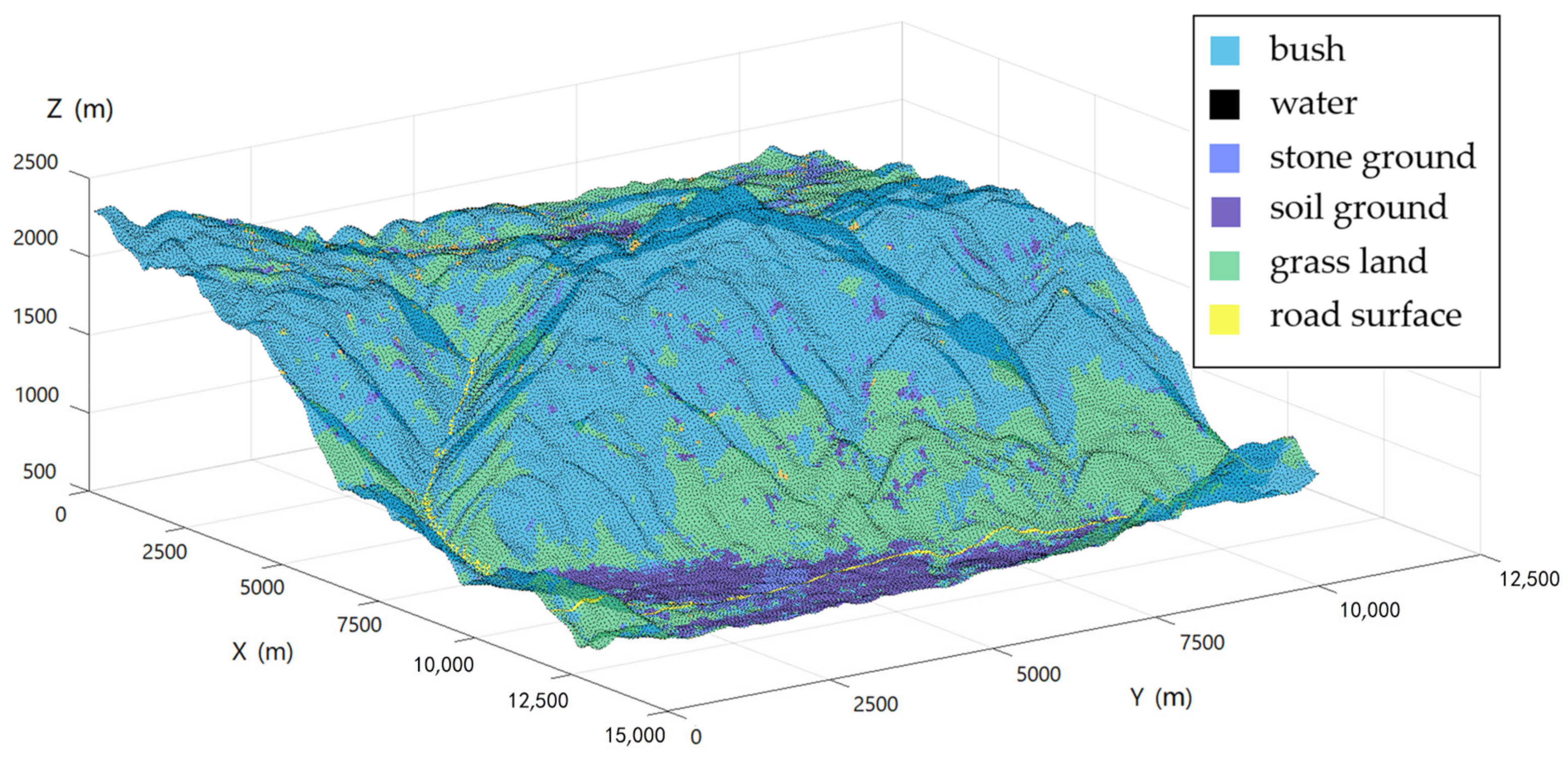
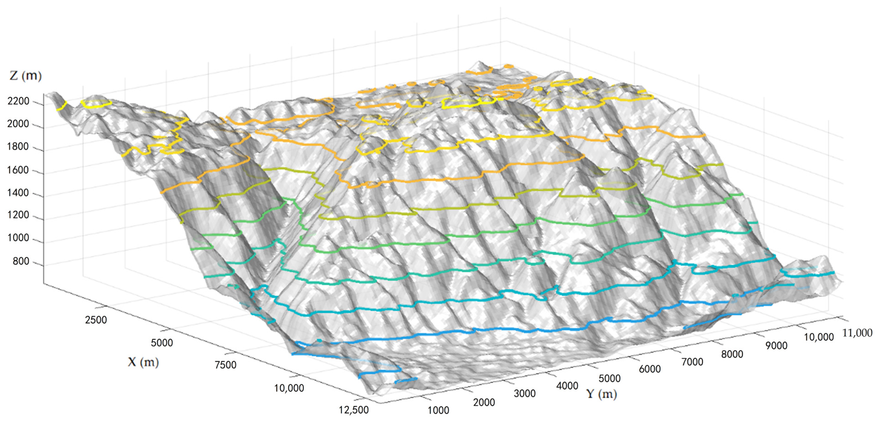
2.1. Study Area and Research Data

Changning County, Yunnan Province, China, has a complex terrain, with a highest elevation of 2875.9 m and a lowest elevation of 608 m. Therefore, part of Changning County was taken as the study area. The study area has the characteristics of a complex terrain, diverse landcover types, and distinct elevation levels. It is a specific area that meets the experimental conditions of the algorithm, with data support for the establishment of an experimental environment model. The environmental modeling was conducted based on Landsat-8 remote sensing data and DEM data in the study area. The spatial resolution of Landset-8 remote sensing images is 30 m. In this study, the 543 bands (false color) of Operational Land Imager (OLI) data were used for the classification of landcover. The DEM data were ASTER DEM data with a resolution of 30 m.

Firstly, six landcover types of water, bush, grass land, soil ground, stone ground, and road surface were obtained from remote sensing images through a supervised classification method [40]. Then, the two kinds of data were spatially connected to obtain the original data including 3D coordinates and landcover information.

As shown in Figure 1a, grid coordinate mapping was carried out on the above original data to realize the establishment of the experimental environment model [41]. This method has the advantages of simple data structure, convenient spatial analysis, and combination of multi-level spatial data. The processed map is still a traditional single-layer map, and its access and reading are in single-interface mode. For this study, the simple data structure was improved by referring to the literature [42]. A multi-layer feature map was constructed to store landcover information and 3D coordinate information (Figure 1b), which could retain environmental feature information effectively and improve the maintainability of the cost map. The resulting landcover distribution and terrain information are shown in Figure 2 and Figure 3, respectively.

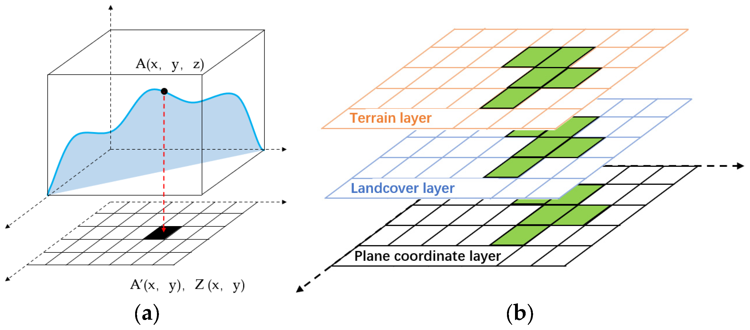
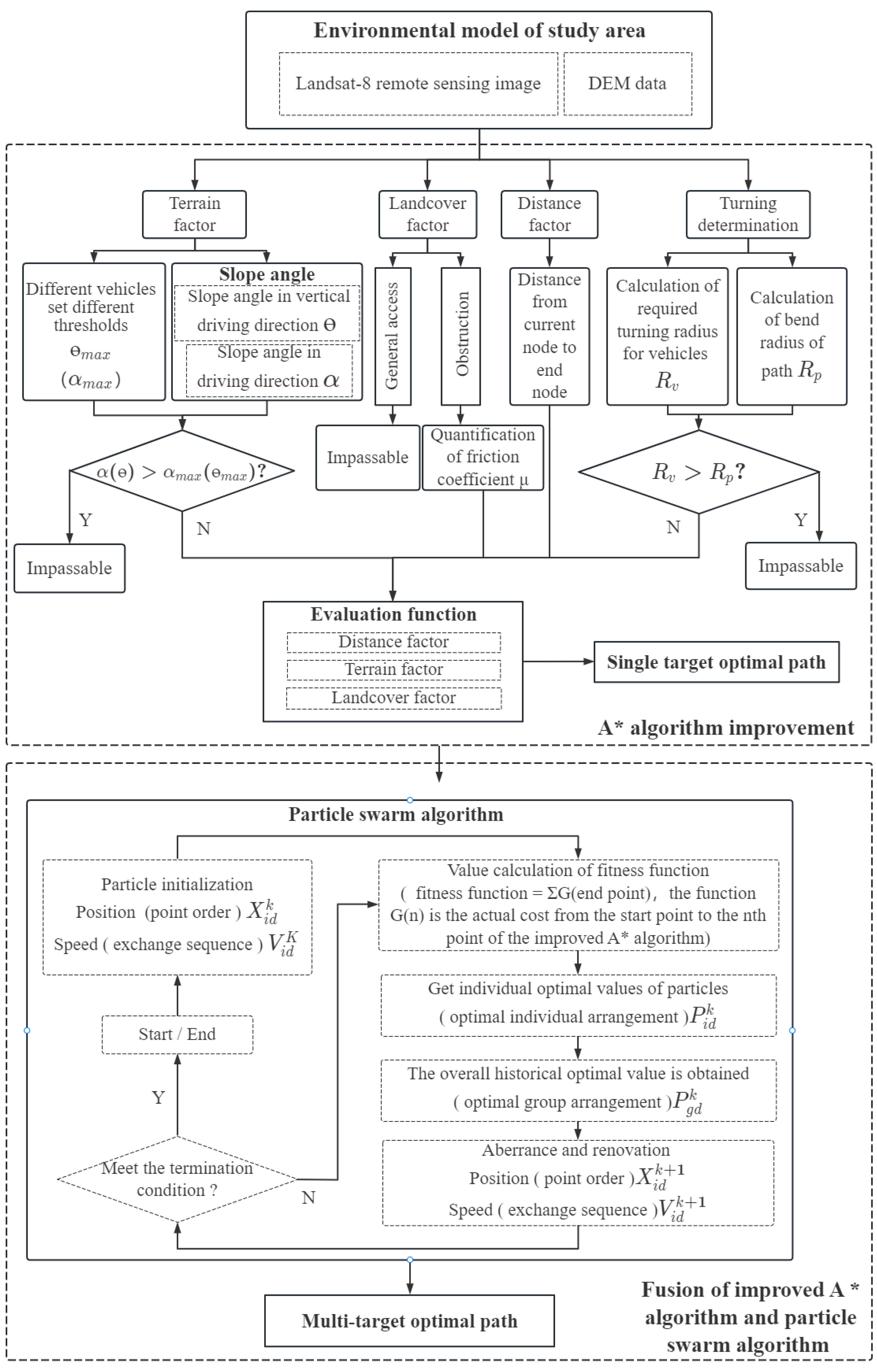
2.2. Technical Route

The landcover factor and terrain factor were added to the evaluation function of the A* algorithm for application in complex field scenes. In addition, the turning radius factor and the slope threshold were taken as judgment conditions of impassable points. Finally, the improved A* algorithm was used as the fitness function of the particle swarm algorithm for an algorithm fusion to solve the TSP. Figure 4 shows the technical road for this paper.

2.3. A* Algorithm Improvement

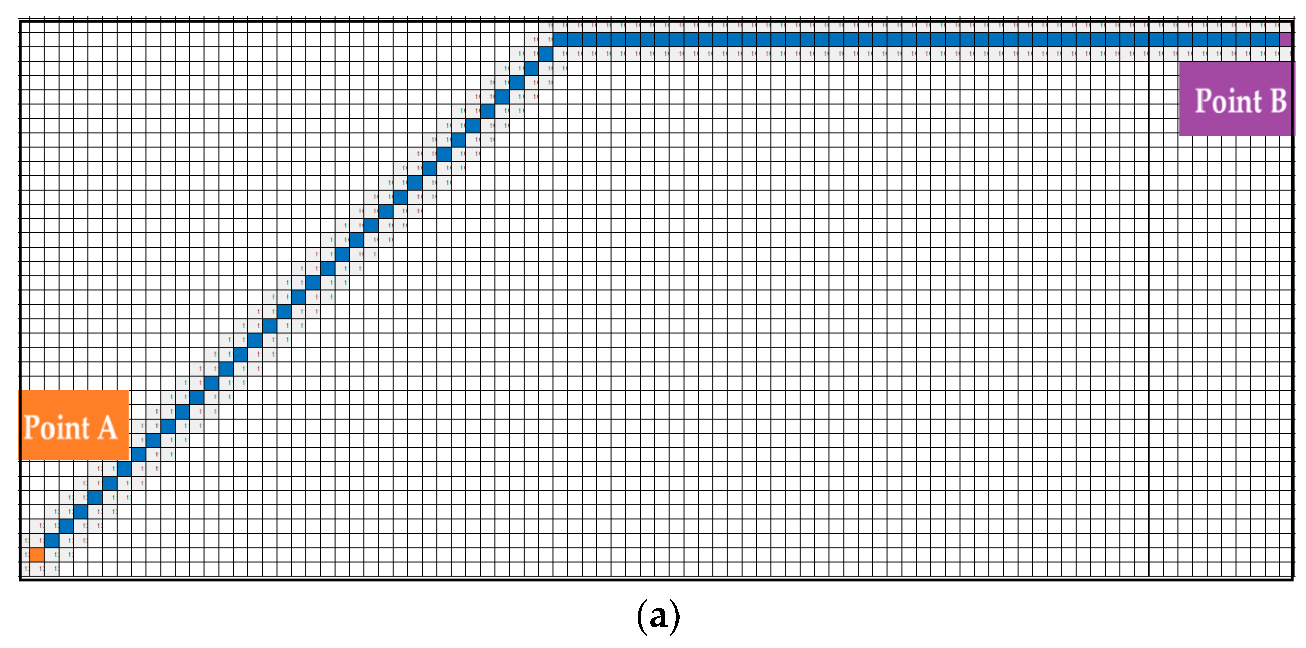
2.3.1. Traditional A* Algorithm

The A* algorithm originates from the Dijkstra algorithm and is a classical and efficient heuristic algorithm. The A* algorithm searches by node and expands by 8 nodes, 24 nodes, etc. In this study, raster coordinate mapping was used as the search map, so eight-node expansion was selected to improve the computational efficiency. Formula (1) is its evaluation function [43,44,45].

$$F\left(n\right)=G\left(n\right)+H\left(n\right),$$

(1)

$$G\left(n\right)=G^{\prime }+\sqrt{{\left(x_n-x_{n-1}\right)}^2+{\left(y_n-y_{n-1}\right)}^2}$$

(2)

$$H\left(n\right)=\sqrt{{\left(x_t-x_n\right)}^2+{\left(y_t-y_n\right)}^2}$$

(3)

where $F\left(n\right)$ is the sum of estimated costs from the starting node, through the current node $n$ and reaching the target; $G\left(n\right)$ is the actual cost from the starting node to the current node $n$; $H\left(n\right)$ is the estimated cost from the current node $n$ to the target node; $G^{\prime }$ represents the original cost from the previous node to the original node; ($x_n, y_n$) is the current node; ($x_{n-1}, y_{n-1}$) is the previous node; and ($x_t, y_t)$ is the target node.

2.3.2. Improvement of the Evaluation Function

Path terrain and landcover are important factors that affect the energy consumption of vehicles. In this study, in order to achieve lower energy consumption in the path planning results, the evaluation function of the traditional A* algorithm was modified by adding the slope parameter and friction factor. The improved A* algorithm was then more inclined toward results with a gentle slope, a small friction factor, and a short total distance when selecting extending nodes. Furthermore, the turning radius factor and slope threshold parameter were added to the definition of impassable points in the A* algorithm. When the path bend of the extending node was less than the minimum turning angle of the vehicle, the node would be added to the list of impassable nodes. Similarly, the path slope cannot be greater than the slope threshold that the vehicle can pass; otherwise, it is also regarded as an impassable node. The friction coefficient was positively correlated with slope value and energy consumption under the condition of equal distance. The improved A* algorithm ensures the trafficability of the path and ensures that the path planning results follow a trend of lower consumption.

The form of the improved evaluation function parameters $G\left(n\right)$ and $H\left(n\right)$ is set as follows:

$$G\left(n\right)=G^{\prime }+\mathrm{Cost}\sqrt{{\left(x_n-x_{n-1}\right)}^2+{\left(y_n-y_{n-1}\right)}^2},$$

(4)

$$H\left(n\right)=\mathrm{Cost}\sqrt{{\left(x_t-x_n\right)}^2+{\left(y_t-y_n\right)}^2},$$

(5)

$$Cost=V_{\theta }\left(Cos{t}_1+Cos{t}_2\right),$$

(6)

$$Cos{t}_1=\mu mg{D}_{cos},$$

(7)

$$Cos{t}_2=mg{D}_{sin},$$

(8)

$$\left\{\begin{array}{c}{V}_{\theta }=1, \left(\mathrm{O}°\le \theta <15°\right) \\ V_{\theta }=2, \left(15°\le \theta <30°\right)\\ V_{\theta }=3, \left(30°\le \theta \le 45°\right),\end{array}\right.$$

(9)

where $G^{\prime }$ represents the original cost from the previous node to the original node, $\mathrm{Cos}\mathrm{t}$ represents the consumption cost coefficient, ($x_n, y_n$) is the current node, ($x_{n-1}, y_{n-1}$) is the previous node, ($x_t, y_t)$ is the target node, $Cos{t}_1$ is the friction factor consumption parameter, $Cos{t}_2$ is the slope consumption parameter in the driving direction, $\alpha$ is the slope angle in the driving direction, $V_{\theta }$ is the slope consumption parameter in the vertical driving direction, $\mu$ is the landcover friction coefficient (according to the landcover type), $m$ is the mass of the vehicle (m is set to mean values for a certain type of vehicle), $g$ is acceleration due to gravity, and $\theta$ is the slope angle of the vertical driving direction.

The parameter $\mu$ in Formula (7) enables the A* algorithm to reflect landcover in its 3D path planning. Different landcover features have different friction coefficients. The landcover of the study area was divided into six types by a supervised classification method: road surface, soil ground, grass land, stone ground, bush, and water. The water was set as an impassable area, and different friction coefficients were set for the landcover types in the passable areas according to the degree of energy consumption [42,46,47]. The landcover friction coefficients are shown in

Table 1. Landcover friction coefficients.

Landcover	Friction Coefficient (µ)	Passable/Impassable
Road surface	0.1	Passable
Soil ground	0.4	Passable
Grass land	0.5	Passable
Stone ground	0.8	Passable
Bush	0.9	Passable
Water	/	Impassable

.

2.3.3. Determination of Impassable Points

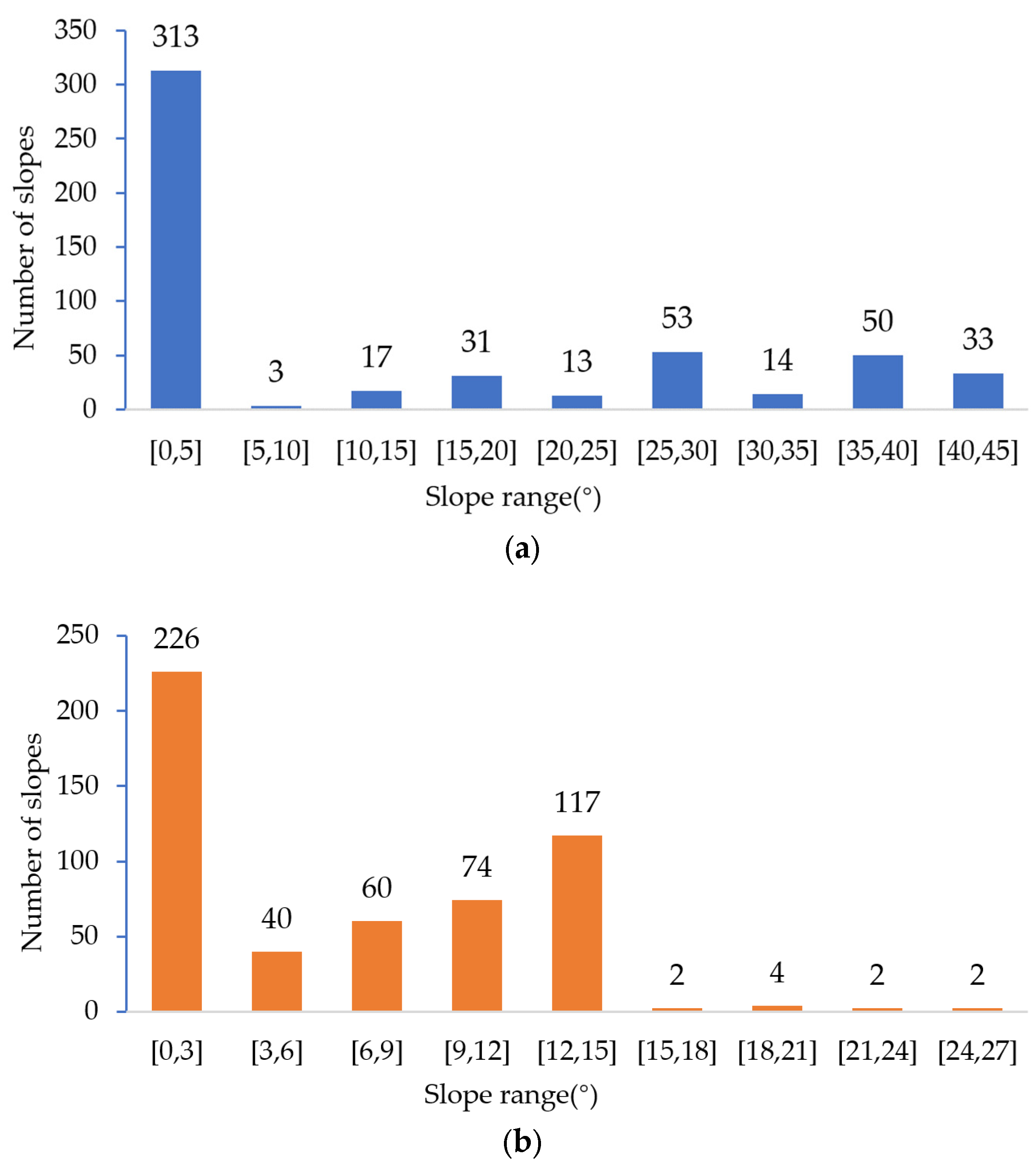
Different access conditions were set for different vehicles (medium vehicle, large vehicle). When the radii of the inner and outer rings of the path are greater than the radii of the inner and outer rings required by the vehicle to turn, it is deemed to be passable; otherwise, it is deemed to be impassable. When the slope of the path is less than the slope threshold that the vehicle can pass, it is deemed to be passable; otherwise, it is deemed to be impassable.

Slope Threshold

The slope angle in the driving direction was divided into ascent and descent, and different maximum passing slopes were set for different vehicles. The slope parameters are shown in

Table 2. Passing slope in the driving direction.

Subject	Type	Passable Range	Impassable Range
Medium vehicle	Ascent	(0°, 45°)	(45°, 90°)
	Descent	(0°, 50°)	(50°, 90°)
Large vehicle	Ascent	(0°, 25°)	(25°, 90°)
	Descent	(0°, 30°)	(30°, 90°)

.

The passable range of slope in the vertical driving direction is (0°, 30°).

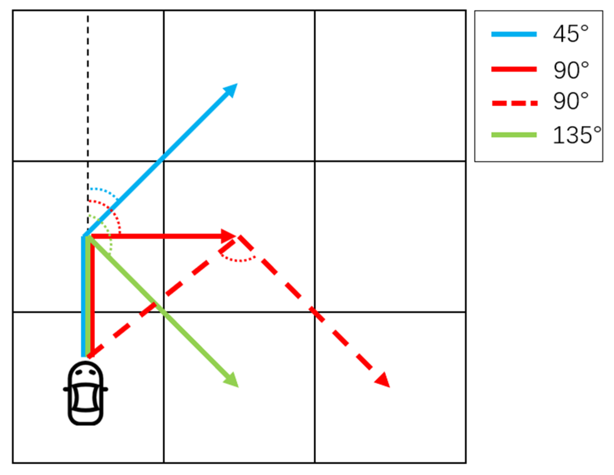
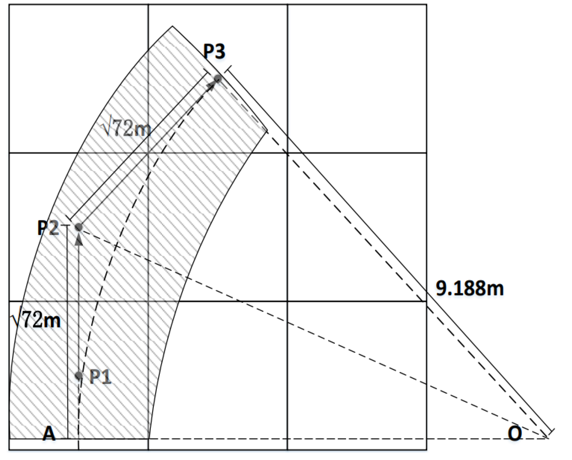
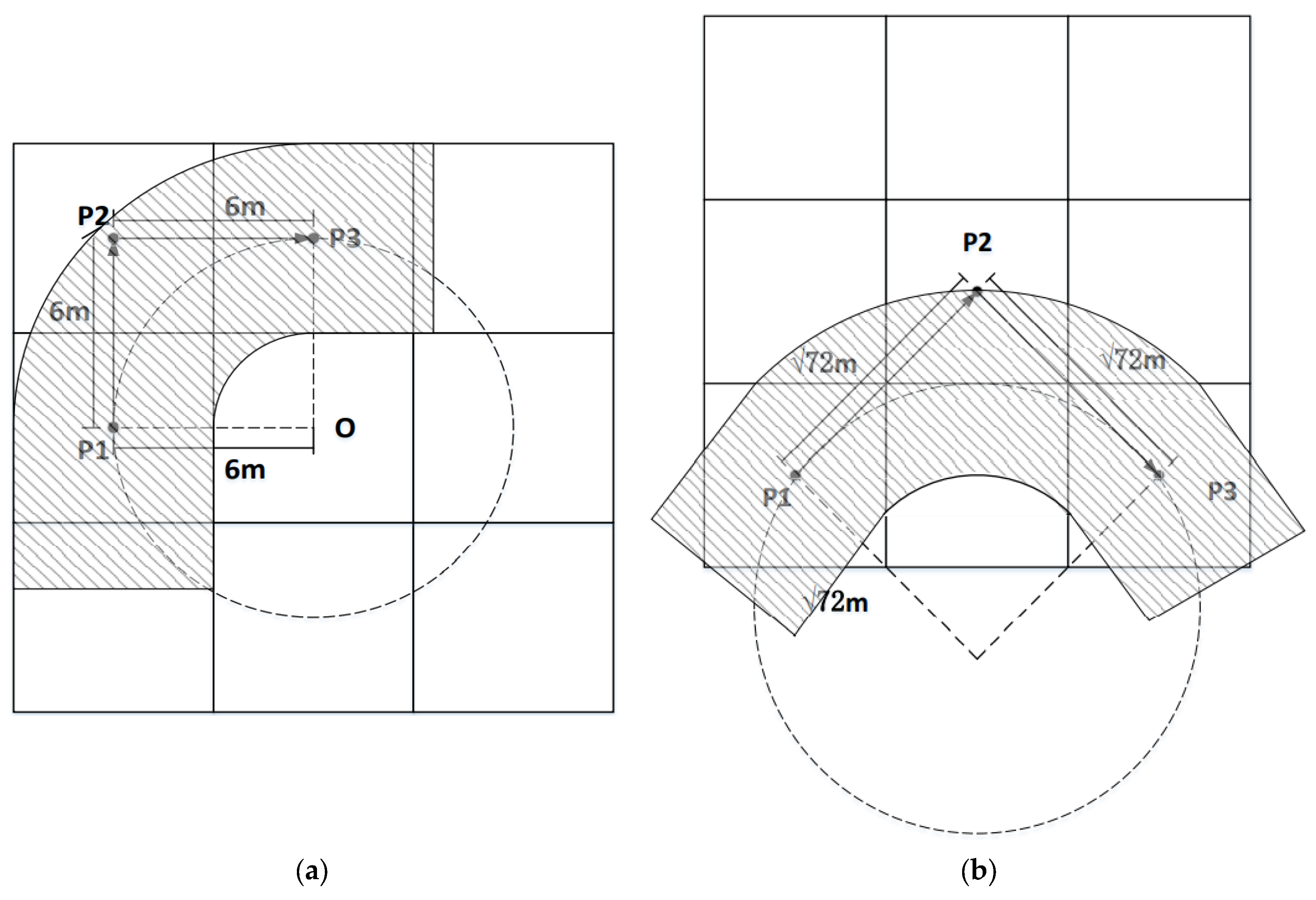
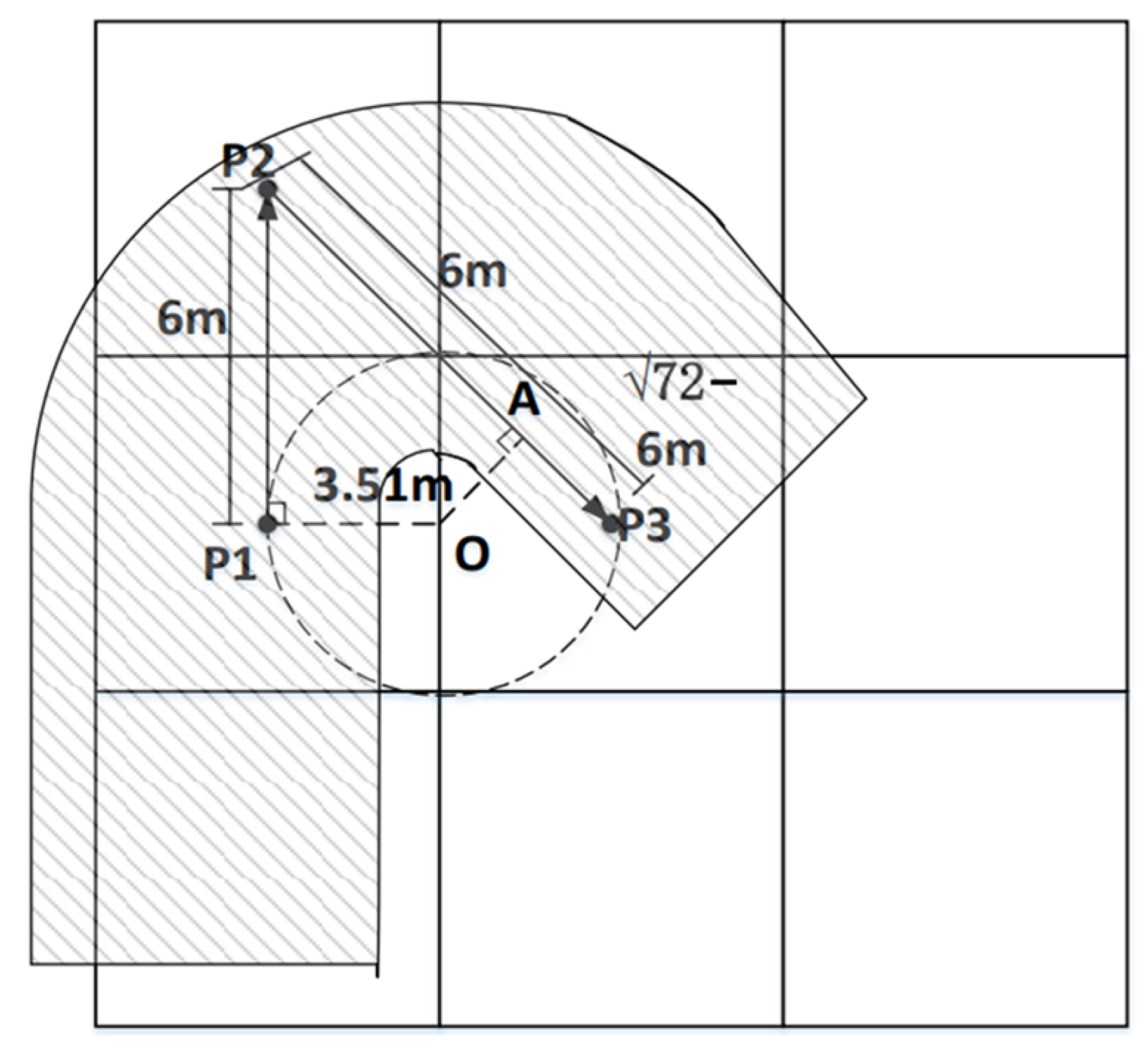
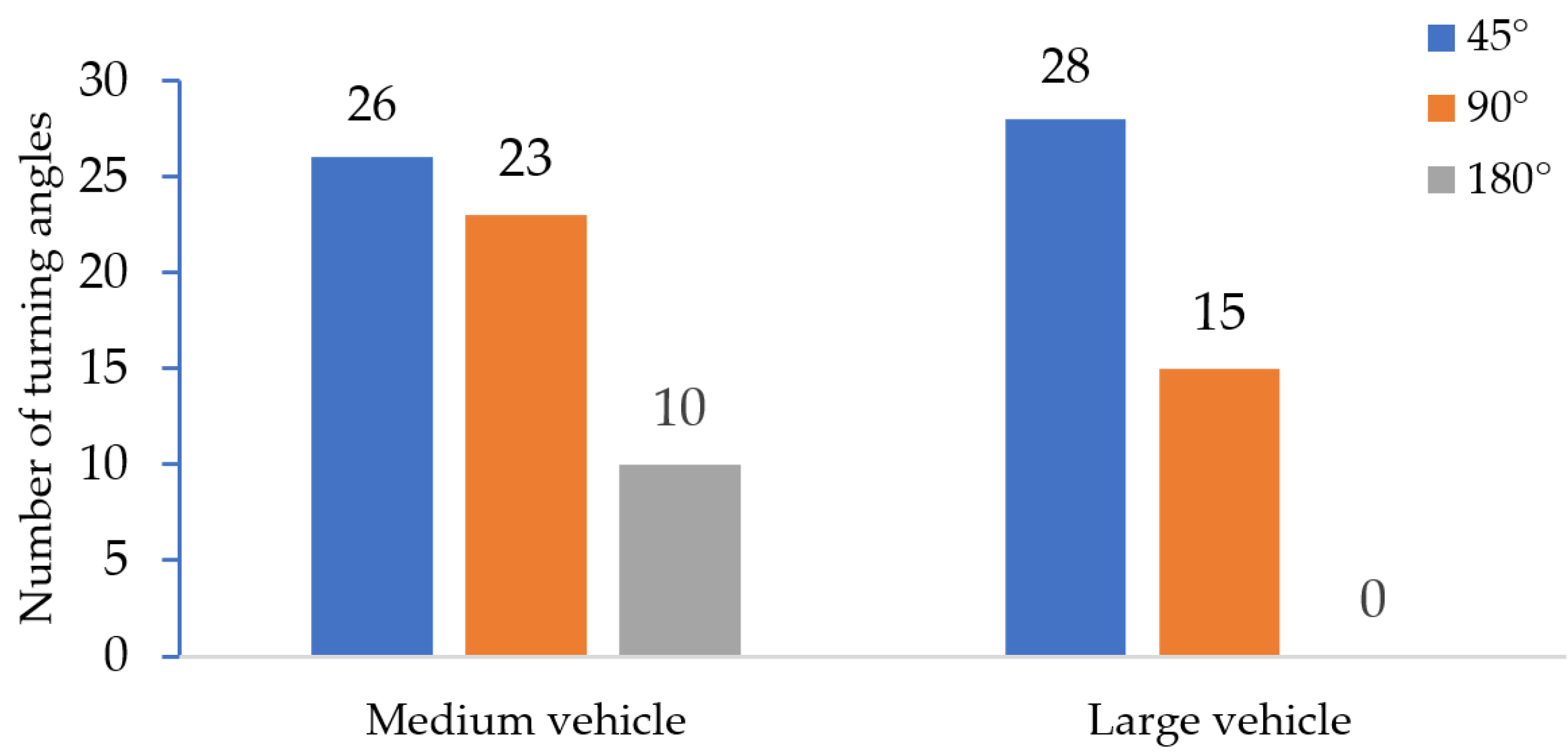
Determination of Turning Angles

In the path planning in this study, eight-node expansion was adopted in the improved A* algorithm, with the eight nodes around each node comprising alternatives for the extending node. The path width was set as a constant, and whether the vehicle (medium or large) can pass a bend of the current width should be considered when selecting the extending node. The radii of the inner and outer rings of the vehicle and the radii of the inner and outer rings of the path are important parameters to judge whether a bend can be passed (Table 3). When the path radii (inner and outer) are larger than the vehicle radii (inner and outer), the node is regarded as passable.

The turning radii of the inner and outer rings of the vehicle were determined by the specific production parameters of the vehicle:

$$r=\sqrt{r_1^2-L^2}-\frac{b+n}{2},$$

(10)

$$r_v=r-y,$$

(11)

$$R=\sqrt{{(L+d)}^2+{(r+b)}^2},$$

(12)

$$R_v=R+x,$$

(13)

where $r$ is the inner radius of the vehicle ring, $r_1$ is the minimum turning radius of the vehicle, $L$ is the axle distance, $b$ is the vehicle width, $n$ is the front wheel distance, $r_{\mathrm{v}}$ is the inner radius of the vehicle ring with the safe distance, $y$ is the inner safe distance, $R$ is the outer radius of the vehicle ring, $d$ is the front suspension ruler length, $R_v$ is the outer radius of the vehicle ring with the safe distance, and $x$ is the outer safety distance [44].

The radii of the inner and outer rings of the path ($r_p$ and $R_p$) turn were determined by the spatial relationship between the starting node and ending node that the vehicle passed through. Thus, there are three situations as follows in Figure 5.

(1)

A 45° angle

As shown in Figure 6, the path is parent node(P₁) → current node(P₂) → child node(P₃), and the vehicle turns 45°. The lengths of connection lines P₁P₂ and P₂P₃ are different, and the turning angle is small. The analysis shows that the turning radius should be controlled by the longer line. Therefore, AP₂ with the same length as P₂P₃ is taken on the P₁P₂ extension line, and points A and P₃ are taken as the perpendiculars of the two lines, respectively. The two perpendiculars intersect at point O, where point O is the center of the circle, and OP₁ is the radius of the circle.

Because OP₁⊥P₁P₂, OP₂ is the angular bisector of ∠P₁P₂P₃; it is then clear that ∠P₁P₂P₃ = 135°°, so ∠P₁P₂O = 67.5°. According to the triangle tangent theorem, the circle radius is $O{P}_1=d\tan ({67.5}^{\circ })$. The radius OP₁ is reduced 3 m inward to form the inner ring radius of the path, while it is extended 3 m outward to form the outer ring radius of the path.

(2)

A 90° angle

As shown in Figure 7a, the path is parent node(P₁) → current node(P₂) → child node(P₃), and the vehicle turns 90°. In order to calculate the internal and external radii of the path in this case, P₁P₂ and P₂P₃ are crossed, and P₁ and P₃ are taken as the respective perpendiculars. The two perpendiculars intersect at point O, and point O is taken as the center of the circle. OP₁ is taken as the radius of the circle. It is clear that the radius of the circle is the same length as the grid edge (6 m), and the circle is extended to the inside and outside by 3 m to form the internal radius and the external radius.

The second situation of a vehicle turning 90° is shown in Figure 7b. The vehicle path is parent node(P₁) → current node(P₂) → child node(P₃), but the radius of the path is longer. The method is the same as that above to obtain a circle of radius $\sqrt{72}$.

(3)

A 135° angle

As shown in Figure 8, the path is parent node(P₁) → current node(P₂) → child node(P₃), and the vehicle turns 135°. The lengths of the connections P₁P₂ and P₂P₃ are different, and the turning angle is large. The analysis shows that the turning radius should be controlled by the short line. Therefore, AP₂ with the same length as P₁P₂ is taken on the line P₂P₃, and points A and P₁ are taken as the respective perpendiculars of the two lines. The two perpendiculars intersect at point O, and point O is taken as the center of the circle; OP₁ is then taken as the radius of the circle. It is clear that ∠P₂P₃P₁ = 45° and OA⊥AP₃, so OP₃ = AP₃ = √72−6; thus, OP₁ = 12−$\sqrt{72}$, about 3.51 m. The circle is extended outside by 4.5 m as the $R_p$ and inside by 1.5 m as the $r_p$.

Using the above methods and the production parameters of all kinds of vehicles, the table of turning coefficients is as follows.

Table 3. Turning radius factors.

Vehicle Type	Middle Vehicle			Large Vehicle
Vehicle name	BAIC Warrior	Range Rover	Rover Evoque	Antiriot fire water tank truck	Fire sprinkler	Foam fire truck
Minimum turning radius of the vehicle (m)	5.280	5.280	4.760	6.026	5.663	6.952
Inner radius of the vehicle ring (m)	2.793	2.443	2.146	2.415	2.121	3.415
Outer radius of the vehicle ring (m)	4.881	5.138	4.604	6.300	6.101	6.908

Table 3. Turning radius factors.

Vehicle Type	Middle Vehicle			Large Vehicle
Vehicle name	BAIC Warrior	Range Rover	Rover Evoque	Antiriot fire water tank truck	Fire sprinkler	Foam fire truck
Minimum turning radius of the vehicle (m)	5.280	5.280	4.760	6.026	5.663	6.952
Inner radius of the vehicle ring (m)	2.793	2.443	2.146	2.415	2.121	3.415
Outer radius of the vehicle ring (m)	4.881	5.138	4.604	6.300	6.101	6.908

2.4. Fusion of the Improved A * Algorithm and Particle Swarm Algorithm

The improved A* algorithm solves the optimal path problem between the starting point and the target point, but it cannot handle the needs of path planning with multi-target points. The problem of path planning with multiple targets is essentially a TSP; the TSP is a non-deterministic polynomial hard problem in combinatorial optimization. This section studies the fusion of the improved A* algorithm and the particle swarm algorithm to solve the TSP.

2.4.1. Implementation of Particle Swarm Algorithm

The logic of the particle swarm algorithm is to generate N-many particles (the number of particles is determined by the number of target points). Each particle is given a random initial position, and the position is updated with speed. After a certain number of iterations (the number of iterations is determined by the number of target points), the optimal position is obtained [48,49]. Formula (14) is the speed update formula, and formula (15) is the position update formula [14]:

$$V_{id}^{k+1}=\omega V_{id}^k+c_1{r}_1\left(P_{id}^k-X_{id}^k\right)+c_2{r}_2\left(P_{gd}^k-X_{id}^k\right),$$

(14)

$$X_{id}^{k+1}=X_{id}^k+V_{id}^{k+1},$$

(15)

where k and k + 1 represent the kth iteration and k + 1 iteration, respectively, $V_{id}^{k+1}$ is the individual particle speed after an iteration, $\omega$ is the inertia factor, $V_{id}^k$ is the individual particle speed before the iteration, $c_1=2$ is the individual learning factor, $r_1$ is a random number, $P_{id}^k$ is the optimal position of the individual, $X_{id}^k$ is the individual particle position before the iteration, $c_2=2$ is the group learning factor, and $r_2$ is a random number. $P_{gd}^k$ is the group optimal position and $X_{id}^{k+1}$ is the particle position after the iteration.

The implementation steps of the particle swarm algorithm are as follows:

• Step 1: Initialize the particle swarm, including random position and speed.
• Step 2: Evaluate the fitness of each particle based on the fitness function.
• Step 3: Determine the individual optimal values of particles, compare the fitness value of each particle with its best position $P_{id}^k$, and then update its best position $P_{id}^k$.
• Step 4: Determine the group optimal value of the particle swarm, compare the current best position $P_{id}^k$ of all particles, and then update the best position $P_{gd}^k$ of the group.
• Step 5: Update the particle speed and position according to formulae (14) and (15).
• Step 6: Return to Step 2 if the end condition is not met.

2.4.2. The Fused Algorithm to Solve TSP

The following pseudocode describes the process of solving TSP by fusing the particle swarm algorithm with the improved A* algorithm (Algorithm 1).

Algorithm 1 The pseudocode of fused algorithm

Particle swarm algorithm and A* algorithm fusion Input: Set of target points Output: Optimal access sequence Begin: (1) for each combination i do % A combination of any two of the nine target points (2) Get the optimal path between two points; (3) Calculate the consumption value $Cos{t}_i$; (4) endfor (5) for each particle i do (6) $X_i$ <- particle initial position, <- particle initial speed; (7) fitness(Xi) <- $\sum _{j=1}^{8}Cos{t}_j$; % $Cos{t}_j$ calculated by the improved A* algorithm (8) Evaluate particle i by fitness(Xi); (9) pBest <- Xi; % Individual optimal value (10) endfor (11) gBest <- min{pBest}; % Group optimal value (12) while not stop do (13) for i <- 1 in number of particles do (14) Update the speed and position of particle i; (15) Calculate fitness(Xi) and evaluate particle i; (16) Update the pBest and the gBest; (17) endfor (18) end while (19) renturn gBest End

In this study, the dimension of path planning was set to nine, and the number of particles was set to 20. According to the results of multiple experiments, convergence could be achieved in most experiments when the number of iterations was in the (15,40) range, so the maximum number of iterations was set at 100 to ensure the optimal solution. In order to avoid falling into the local optimal solution as much as possible, the nonlinear decreasing weight was used in this study and calculated as follows:

$$w=w_i-\left(w_i-w_m\right)\ast {\left(\frac{g_k}{g_m}\right)}^2,$$

(16)

where $w_i=0.9$ is the initial inertia weight, $w_m=0.4$ is the inertia weight of the maximum number of iterations, $g_k$ is the current iteration algebra, and $g_m$ is the maximum iteration number determined.

Calculating the fitness value of the particle in the pseudocode is actually to get the energy consumption value of the vehicle under the access sequence of the target point. The total consumption can be obtained by successively summing the consumption values between the two target points in the access sequence. The improved A* algorithm serves as the fitness function’s foundation in this study. The total consumption cost as per Formulas (4) and (5) were applied to calculate the fitness value. The minimum-consumption-value path order selected in this iteration was taken as the group optimal solution of the current iteration, and the individual optimal solution of each particle was updated in each iteration. After several iterations, the global optimal solution was obtained. Using this calculation method, the multi-target path planning standard can not only consider the distance factor but also comprehensively consider the terrain and landcover.

3. Results and Analysis

In this paper, the path planning is simulated in the MATALAB R2018b environment and is run on a server with a 2.60 GHz CPU, 32.00 GB of RAM, and Window10 $\times 64$ operating system.

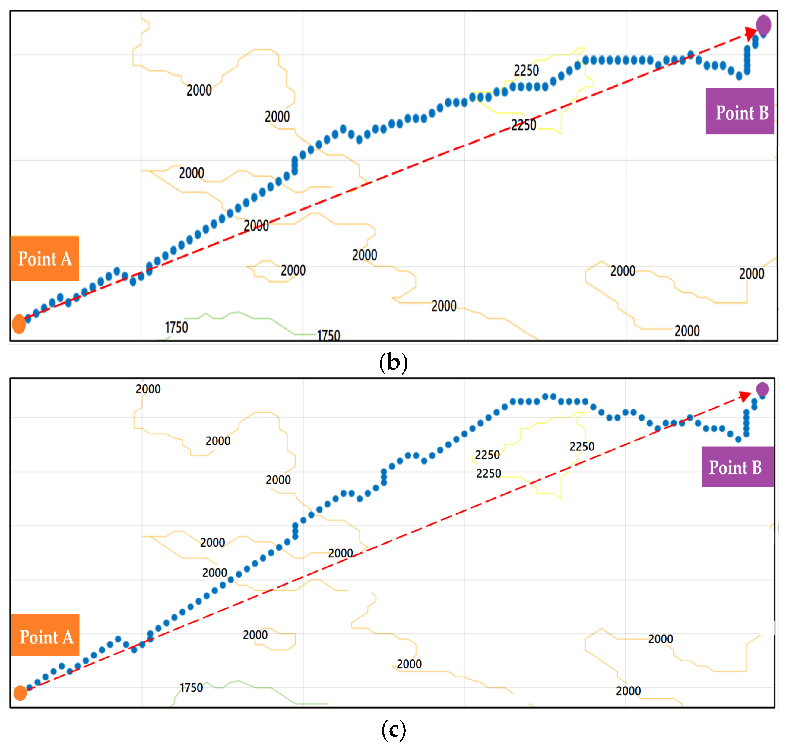
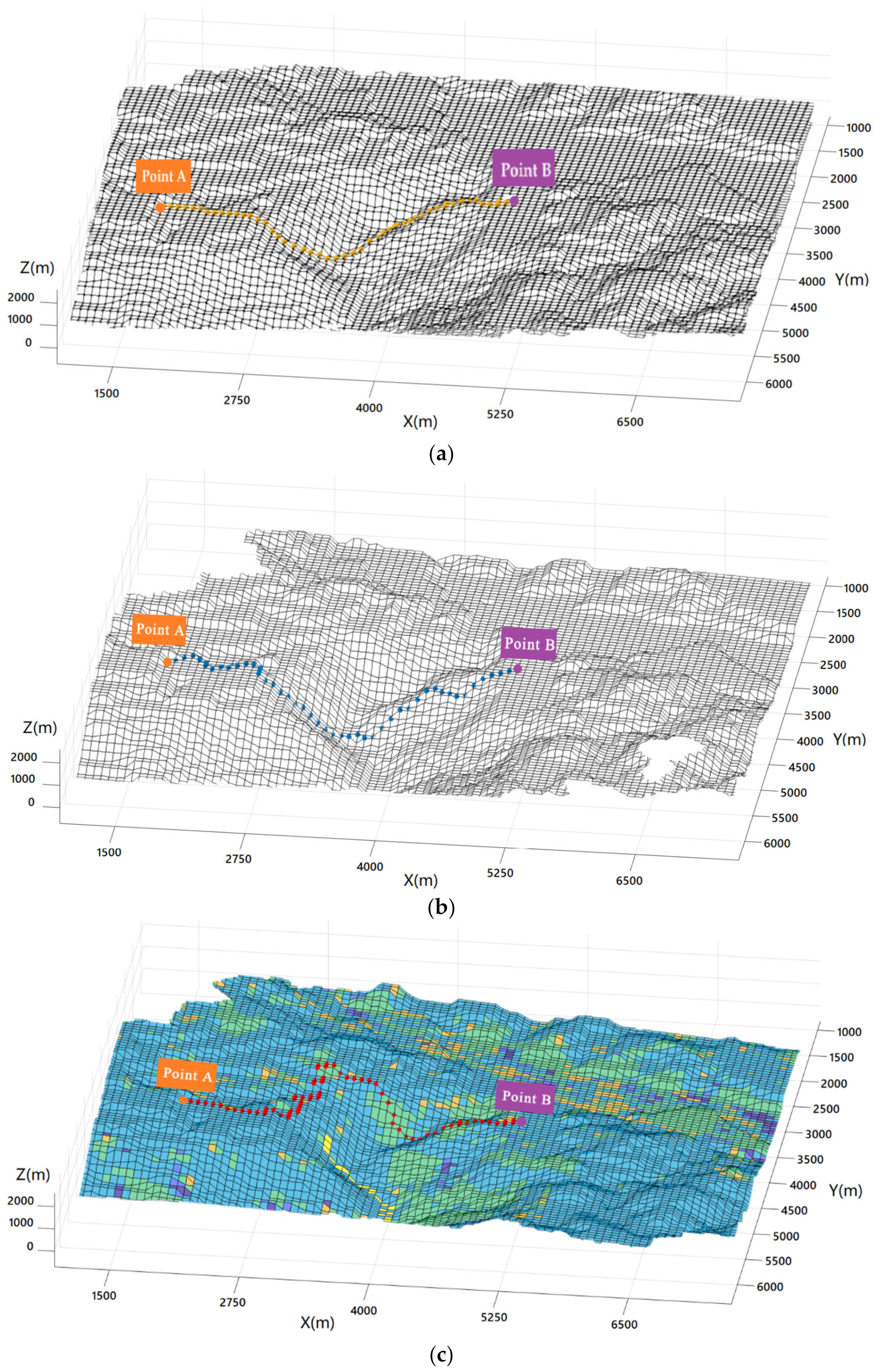
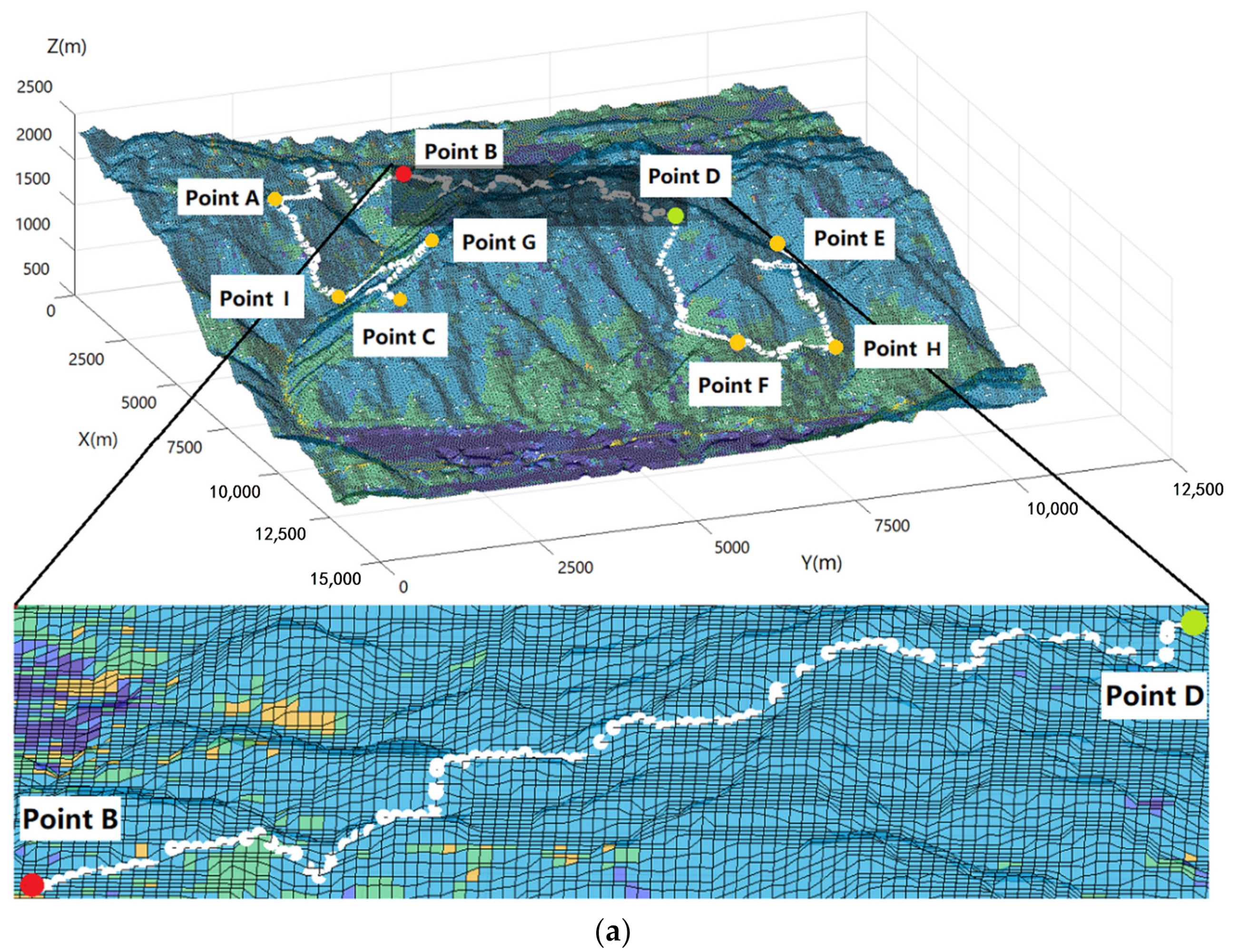
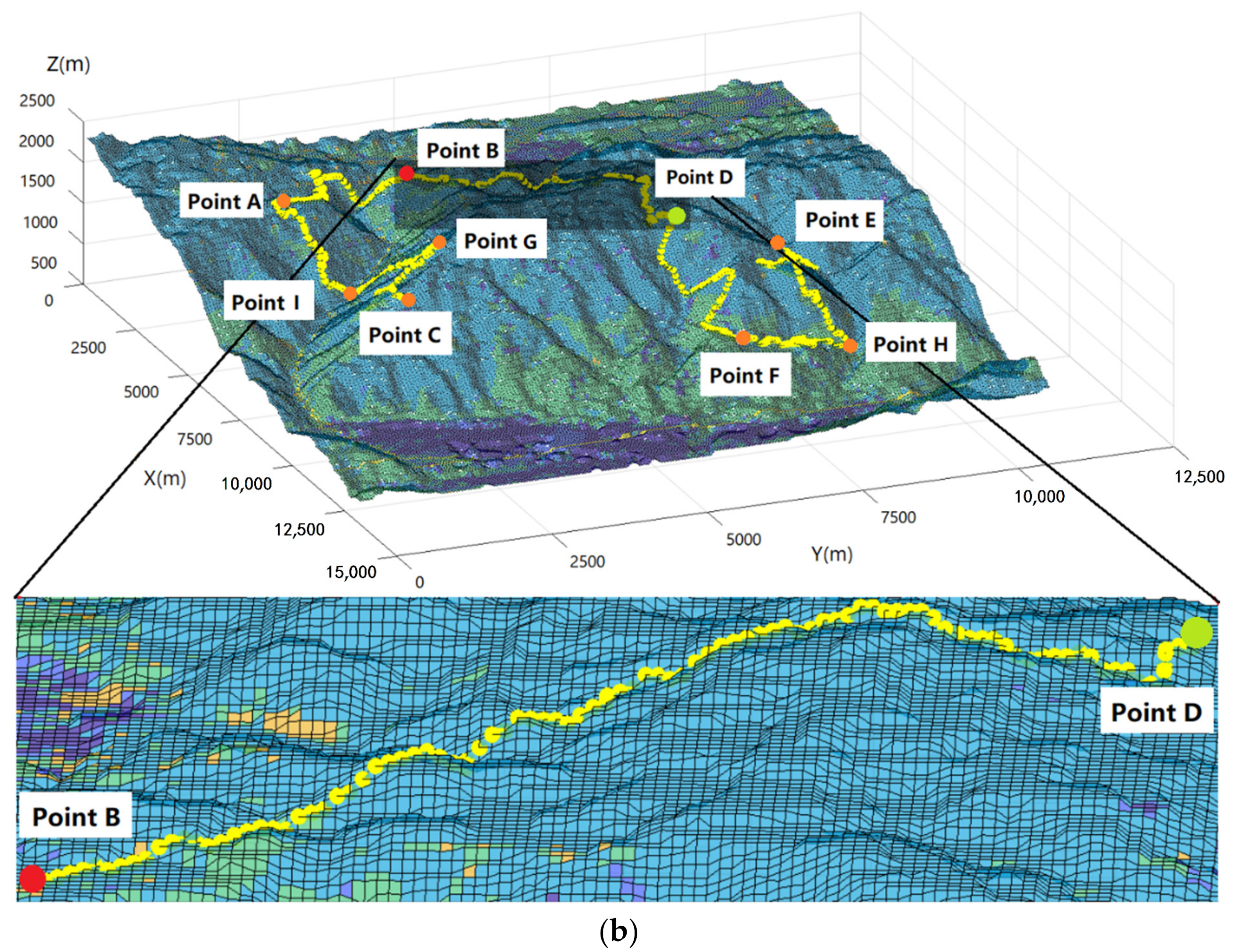
3.1. The Effect of Terrain on the A* Algorithm

This section discusses the effect of terrain factors on path planning results with the improved A* algorithm. In Figure 9, for medium vehicles, three kinds of path planning results (A→B) are obtained by using different forms of the A* algorithm (traditional A*, including land cover but not terrain, and including land cover and terrain). Figure 9a shows the path planning results of the traditional A* algorithm for two points, A and B, in the plane model. In the 3D model, the planned path in Figure 9b crosses the 2250 m contour line, while the planned path in Figure 9c can bypass the area with steep terrain.

It can be seen from the experimental results that when the A* algorithm is extended to the 3D model, the results are different due to the different distance calculation methods. Furthermore, because the evaluation criterion in the evaluation function is the minimum total energy consumption and the vehicle must overcome gravity to do work in the uphill process, in contrast to Figure 9b,c considers terrain when improving the A* algorithm, resulting in a gentler path slope.

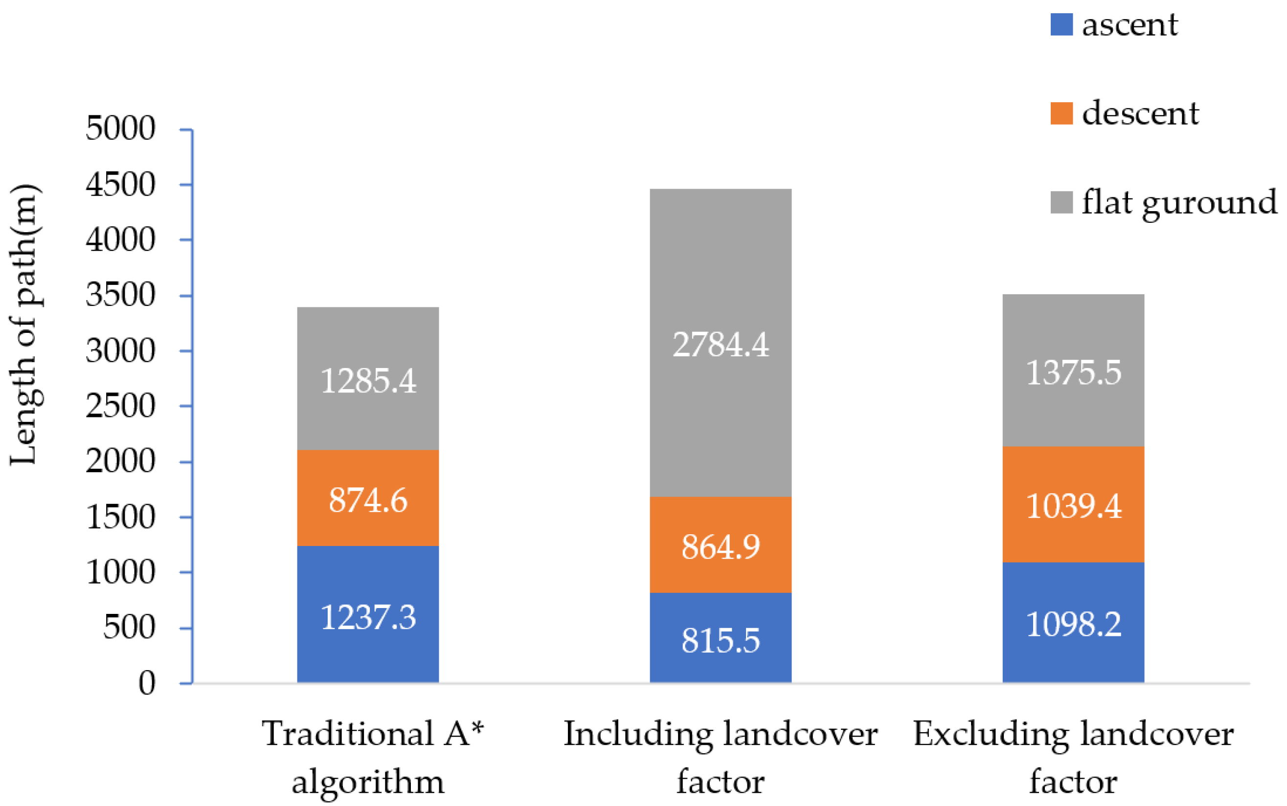
3.2. The Effect of Landcover on the A* Algorithm

This section discusses the effect of landcover factors on path planning results with the improved A* algorithm. In Figure 10, two planned paths (A→B) are represented for medium vehicles, obtained by the different A* algorithm forms (traditional A* algorithm in 3D model, including terrain but excluding landcover, including both terrain and landcover).

The path planning extended by the traditional A* algorithm to the 3D model is shown in Figure 10a. Its evaluation function takes into account only the spatial distance between nodes. As a result, unlike Figure 10b, Figure 10a cannot avoid nodes with a steeper slope. The path shown in Figure 10b took into account both the distance factor and the terrain factor between the two target points, while the path in Figure 10c took only landcover into consideration. The planned path was inclined to choose soil ground rather than bush because μ_{soil ground} (0.4) was far less than μ_bush (0.9) in this study. In other words, the path planning result was affected by the friction coefficient when the landcover factor was added to the A* algorithm. From a distance perspective (Figure 11), the total length of the path in Figure 10b is 3513.1 m; this is less than the length of the path in Figure 10c, which is 4464.8 m. However, when considering the work done by the vehicle to overcome the friction force (taking the landcover friction coefficient set in this study instead of the actual rolling friction coefficient) and gravity, the energy consumption by the vehicles is 4.21 × 10⁷ J in Figure 10b and 3.15 × 10⁷ J in Figure 10c (Table 4). It can thus be concluded that the planned path, considering landcover factors, would lead to lower energy consumption for vehicles. The energy-saving efficiency statistics of the path planning results of the improved algorithm (three representative paths) are shown in Table 5. In total, the average energy-saving efficiency of the improved algorithm is 14.7%.

Figure 11. Path length statistics.

Figure 11. Path length statistics.

Table 4. Statistical results of path planning experiments.

Path Planning Result Parameter	Experiment (a) Traditional A* Algorithm	Experiment (b) Excluding Landcover	Experiment (c) Including Landcover
Path length (m)	3397.3	3513.1	4464.8
Soil ground (m)	811.4	843.1	2030.6
Bush (m)	2292.7	2424.3	2134.7
Ascent (m)	1237.3	1098.2	815.3
Descent (m)	874.6	1039.4	864.9
Flat ground (m)	1285.4.	1375.5	2784.4
Energy consumption (J)	4.25 × 107	4.21 × 107$\downarrow$	3.15 × 107$\downarrow$

Table 4. Statistical results of path planning experiments.

Path Planning Result Parameter	Experiment (a) Traditional A* Algorithm	Experiment (b) Excluding Landcover	Experiment (c) Including Landcover
Path length (m)	3397.3	3513.1	4464.8
Soil ground (m)	811.4	843.1	2030.6
Bush (m)	2292.7	2424.3	2134.7
Ascent (m)	1237.3	1098.2	815.3
Descent (m)	874.6	1039.4	864.9
Flat ground (m)	1285.4.	1375.5	2784.4
Energy consumption (J)	4.25 × 107	4.21 × 107$\downarrow$	3.15 × 107$\downarrow$

Table 5. The energy-saving efficiency statistics of the improved algorithm under different paths.

Path	Method	Path Length (m)	Energy Consumption (J)	Energy-Saving Efficiency
A→B	A* algorithm	3397.3	4.25 × 107	/
	Ours	4464.8	3.15 × 107	25.9%
D→F	A* algorithm	4438.2	2.07 × 107	/
	Ours	5010.7	1.85 × 107	10.6%
F→H	A* algorithm	1335.6	1.68 × 107	/
	Ours	1598.7	1.61 × 107	4.7%

(The path is shown in Figure 12).

Table 5. The energy-saving efficiency statistics of the improved algorithm under different paths.

Path	Method	Path Length (m)	Energy Consumption (J)	Energy-Saving Efficiency
A→B	A* algorithm	3397.3	4.25 × 107	/
	Ours	4464.8	3.15 × 107	25.9%
D→F	A* algorithm	4438.2	2.07 × 107	/
	Ours	5010.7	1.85 × 107	10.6%
F→H	A* algorithm	1335.6	1.68 × 107	/
	Ours	1598.7	1.61 × 107	4.7%

(The path is shown in Figure 12).

Figure 12. Multi-target path planning for (a) medium vehicles and (b) large vehicles.

Figure 12. Multi-target path planning for (a) medium vehicles and (b) large vehicles.

3.3. The Effect of Changing the Fitness Function on the Particle Swarm Algorithm

3.3.1. Application of the Fused Particle Swarm Algorithm to the TSP

In order to solve a multi-target path planning problem, the improved A* algorithm was fused with the particle swarm algorithm. According to the actual requirements of the study, the starting point and the end point of TSP are no longer set to coincide in the experiment, and the results given are non-closed paths. Figure 12 displays the respective outcomes of nine points (A, B, C, D, E, F, G, H, I) in 3D path planning for a medium vehicle and a large vehicle, with point C as the starting point and point E as the ending point.

The access order for the target points for the two types of vehicles is C→G→I→A→B→D→F→H→E, as shown in Figure 12. Since the fitness evaluation index of a single particle in each iteration of the particle swarm algorithm is the path consumption cost of the two target points (calculated by the improved A* algorithm), the final access order is the result with the lowest total path consumption.

3.3.2. The Effect of Changing the Fitness Function

Although the target points’ access order was the same, the paths were not (Figure 12a,b). This is due to the different parameters of the two types of vehicles. It can be seen from Section 2.3.3 that the improved A* algorithm alters the slope thresholds and turning conditions for different vehicles.

According to the B→D path marked in Figure 12a,b, the slope angles in the driving direction of a medium vehicle and a large vehicle are presented in Figure 13a,b, respectively. For medium vehicles, the proportion of slope angles in the range [0°,5°] is 59.4%, and the distribution is relatively uniform in the range [5°,45°]. For large vehicles, slope angles in the [0°,3°] range account for 42.9%, and those in the [3°,15°] range account for 55.2%. The result of the two paths corresponds to the reality that the slope threshold and climbing ability of large vehicles are lower than those of medium vehicles.

According to the bend statistics for turning conditions (Figure 14), there were 59 bends for a medium vehicle and 43 bends for a large vehicle. Concretely, the proportions of 45° and 90° turning angles were 44.07% and 38.98%, respectively, for the medium vehicle, while they were 65.12% and 34.88%, respectively, for the large vehicle. Due to the large structure and wheelbase, large vehicles need stricter turning conditions.

3.4. Computational Complexity Analysis of the Algorithm

The improved A* algorithm can work out the minimum consumption path between two arbitrarily chosen target points, and its time complexity is O(n), where n is the number of path nodes. The time complexity of the particle swarm algorithm is O(N*M), where N is the number of iterations and M is the number of particles.

The algorithm’s time frequency could be used to estimate the statement execution times. In the process of algorithm fusion, the improved A* algorithm is used to calculate the cost between any two target points, and then the particle’s fitness is evaluated by the particle swarm algorithm using the results of the improved A* algorithm. Since the improved A* algorithm has eight expansion nodes, the value of F(n) needs to be calculated at most eight times when searching for nodes. According to the pseudocode, the particle swarm algorithm includes updating speed, updating position, calculating particle fitness, updating individual extrema, and updating group extrema in each iteration. Thus, the analysis of computational complexity in this study could be expanded according to the above two complex parts. The computational complexity description is shown in

Table 6. Computational complexity description.

Algorithm	Time Frequency T(n)	Time Complexity O(n)
Improved A* algorithm	47 × n	O(n)
PSO algorithm	26 × N × M + 23 × M	O(N × M)
The fused algorithm	47 × n + 26 × N × M + 23 × M	O(n + N × M)

.

4. Conclusions

In this paper, in order to study the 3D path planning problem in complex field scenes, the A* algorithm was improved and fused with the particle swarm algorithm. In the study area, an experimental environment model was established to apply the algorithm. The conclusions are as follows:

(1)

The terrain factor and landcover factor were added to the evaluation function of the A* algorithm for complex field scenes. The improved A* algorithm can comprehensively analyze the friction coefficient of landcover, the slope value, and the energy consumption in complex field scenes, and it can thus give optimal path planning results. The path planning results have the characteristics of a small friction coefficient, a gentle slope, and energy efficiency. Therefore, the improved A* algorithm in this paper has better adaptability to complex field scenes.

(2)

To ensure path trafficability, stricter restrictions were set on the impassable points in the improved A* algorithm. By studying the turning conditions and the slope of the path, the path planning results can avoid bends and steep slopes that the vehicle cannot pass. Therefore, the improved algorithm ensures that the planned paths for various types of vehicles are passable.

(3)

A fusion of the improved A* algorithm and the particle swarm algorithm was proposed for multi-target 3D path planning in complex field scenes. The fused algorithm effectively realized multi-target path planning, and the optimal access order could meet the requirement of the lowest total path consumption. The result of the fusion algorithm in the multi-target path planning experiment is the route with the lowest energy consumption from the starting point to the end point. The algorithm in this paper produces more energy-efficient vehicle path planning.

Experiments show that the improved path planning algorithm in this study can be applied to navigation in ecological tourism, field geological exploration, and other activities in complex field scenes. The improved algorithm ensures path planning results are passable and energy efficient, and it can effectively reduce the impact of energy supply shortages and adverse traffic in complex field environments.

References

1. Chen, Y.B.; Luo, Y.B.; Mei, Y.S.; Yu, J.Q.; Su, X.L. UAV path planning using artificial potential field updated by optimal control theory. Int. J. Syst. Sci. 2016, 47, 1407–1420. [Google Scholar] [CrossRef]
2. Fan, X.J.; Guo, Y.J.; Liu, H.; Wei, B.W.; Lyu, W.H. Improved Artificial Potential Field Method Applied for AUV Path Planning. Math. Probl. Eng. 2020, 2020, 6523158. [Google Scholar] [CrossRef]
3. Kothari, M.; Postlethwaite, I. A Probabilistically Robust Path Planning Algorithm for UAVs Using Rapidly-Exploring Random Trees. J. Intell. Robot. Syst. 2013, 71, 231–253. [Google Scholar] [CrossRef]
4. Qureshi, A.H.; Ayaz, Y. Intelligent bidirectional rapidly-exploring random trees for optimal motion planning in complex cluttered environments. Robot. Auton. Syst. 2015, 68, 1–11. [Google Scholar] [CrossRef] [Green Version]
5. Pérez-Hurtado, I.; Martínez-Del-Amor, M.; Zhang, G.; Neri, F.; Pérez-Jiménez, M. A membrane parallel rapidly-exploring random tree algorithm for robotic motion planning. Integr. Comput. Aided Eng. 2020, 27, 121–138. [Google Scholar] [CrossRef]
6. Duchon, F.; Babinec, A.; Kajan, M.; Beno, P.; Florek, M.; Fico, T.; Jurisica, L. Path planning with modified A star algorithm for a mobile robot. Model. Mech. Mechatron. Syst. 2014, 96, 59–69. [Google Scholar] [CrossRef] [Green Version]
7. Wang, C.B.; Wang, L.; Qin, J.; Wu, Z.Z.; Duan, L.H. Path Planning of Automated Guided Vehicles Based on Improved A-Star. In Proceedings of the CT IEEE International Conference on Information and Automation, Lijiang, China, 8–10 August 2015. [Google Scholar]
8. Zuo, L.; Guo, Q.; Xu, X.; Fu, H. A hierarchical path planning approach based on A* and least-squares policy iteration for mobile robots. Neurocomputing 2015, 170, 257–266. [Google Scholar] [CrossRef]
9. Katoch, S.; Chauhan, S.S.; Kumar, V. A review on genetic algorithm: Past, present, and future. Multimed. Tools Appl. 2021, 80, 8091–8126. [Google Scholar] [CrossRef]
10. Tuncer, A.; Yildirim, M. Dynamic path planning of mobile robots with improved genetic algorithm. Comput. Electr. Eng. 2012, 38, 1564–1572. [Google Scholar] [CrossRef]
11. Bakdi, A.; Hentout, A.; Boutami, H.; Maoudj, A.; Hachour, O.; Bouzouia, B. Optimal path planning and execution for mobile robots using genetic algorithm and adaptive fuzzy-logic control. Robot. Auton. Syst. 2017, 89, 95–109. [Google Scholar] [CrossRef]
12. Dorigo, M.; Maniezzo, V.; Colorni, A. Ant system: Optimization by a colony of cooperating agents. IEEE Trans. Syst. Man Cybern. Part B-Cybern. 1996, 26, 29–41. [Google Scholar] [CrossRef] [PubMed] [Green Version]
13. Dorigo, M.; Birattari, M.; Stutzle, T. Ant colony optimization—Artificial ants as a computational intelligence technique. IEEE Comput. Intell. Mag. 2006, 1, 28–39. [Google Scholar] [CrossRef]
14. Shi, X.H.; Liang, Y.C.; Lee, H.P.; Lu, C.; Wang, Q.X. Particle swarm optimization-based algorithms for TSP and generalized TSP. Inf. Process. Lett. 2007, 103, 169–176. [Google Scholar] [CrossRef]
15. Xu, G.P.; Cui, Q.L.; Shi, X.H. Particle swarm optimization based on dimensional learning strategy. Swarm Evol. Comput. 2019, 45, 33–51. [Google Scholar] [CrossRef]
16. Zhang, X.; Lin, Q. Three-learning strategy particle swarm algorithm for global optimization problems. Inf. Sci. 2022, 593, 289–313. [Google Scholar] [CrossRef]
17. Yu, J.L.; Su, Y.C.; Liao, Y.F. The Path Planning of Mobile Robot by Neural Networks and Hierarchical Reinforcement Learning. Front. Neurorobotics 2020, 14, 63. [Google Scholar] [CrossRef]
18. Zhang, P.C.; Xiong, C.; Li, W.K.; Du, X.X.; Zhao, C. Path planning for mobile robot based on modified rapidly exploring random tree method and neural network. Int. J. Adv. Robot. Syst. 2018, 15, 1729881418784221. [Google Scholar] [CrossRef] [Green Version]
19. Zhou, C.M.; Huang, B.D.; Franti, P. A review of motion planning algorithms for intelligent robots. J. Intell. Manuf. 2022, 33, 387–424. [Google Scholar] [CrossRef]
20. Lin, S.W.; Liu, A.; Wang, J.G.; Kong, X.Y. A Review of Path-Planning Approaches for Multiple Mobile Robots. Machines 2022, 10, 773. [Google Scholar] [CrossRef]
21. Gong, Y.J.; Li, J.J.; Zhou, Y.C.; Li, Y.; Chung, H.S.H. Genetic Learning Particle Swarm Optimization. IEEE Trans. Cybern. 2016, 46, 2277–2290. [Google Scholar] [CrossRef] [Green Version]
22. Derrac, J.; Garcia, S.; Molina, D.; Herrera, F. A practical tutorial on the use of nonparametric statistical tests as a methodology for comparing evolutionary and swarm intelligence algorithms. Swarm Evol. Comput. 2011, 1, 3–18. [Google Scholar] [CrossRef]
23. Bonyadi, M.R.; Michalewicz, Z. Particle Swarm Optimization for Single Objective Continuous Space Problems: A Review. Evol. Comput. 2017, 25, 1–54. [Google Scholar] [CrossRef]
24. Heidari, A.A.; Mirjalili, S.; Faris, H.; Aljarah, I.; Mafarja, M.; Chen, H.L. Harris hawks optimization: Algorithm and applications. Future Gener. Comput. Syst. Int. J. Escience 2019, 97, 849–872. [Google Scholar] [CrossRef]
25. Coello, C.A.C.; Pulido, G.T.; Lechuga, M.S. Handling multiple objectives with particle swarm optimization. IEEE Trans. Evol. Comput. 2004, 8, 256–279. [Google Scholar] [CrossRef]
26. Ji, W.D.; Wang, J.H.; Zhang, J. An Improved Real Hybrid Genetic Algorithm. Teh. Vjesn. Tech. Gaz. 2014, 21, 979–986. [Google Scholar]
27. Zhan, Z.H.; Zhang, J.; Li, Y.; Chung, H.S.H. Adaptive Particle Swarm Optimization. IEEE Trans. Syst. Man Cybernetics. Part B Cybern. 2009, 39, 1362–1381. [Google Scholar] [CrossRef] [Green Version]
28. Karaman, S.; Frazzoli, E. Sampling-based algorithms for optimal motion planning. Int. J. Robot. Res. 2011, 30, 846–894. [Google Scholar] [CrossRef] [Green Version]
29. Qureshi, A.H.; Mumtaz, S.; Ayaz, Y.; Hasan, O.; Muhammad, M.S.; Mahmood, M.T. Triangular Geometrized Sampling Heuristics for Fast Optimal Motion Planning. Int. J. Adv. Robot. Syst. 2015, 12, 10. [Google Scholar] [CrossRef]
30. Wu, Z.P.; Meng, Z.J.; Zhao, W.L.; Wu, Z. Fast-RRT: A RRT-Based Optimal Path Finding Method. Appl. Sci. 2021, 11, 11777. [Google Scholar] [CrossRef]
31. Tang, G.; Tang, C.Q.; Claramunt, C.; Hu, X.; Zhou, P.P. Geometric A-Star Algorithm: An Improved A-Star Algorithm for AGV Path Planning in a Port Environment. IEEE Access 2021, 9, 59196–59210. [Google Scholar] [CrossRef]
32. Shang, E.K.; Bin, D.; Nie, Y.M.; Qi, Z.; Liang, X.; Zhao, D.W. An improved A-Star based path planning algorithm for autonomous land vehicles. Int. J. Adv. Robot. Syst. 2020, 17, 1729881420962263. [Google Scholar]
33. Zhang, J.; Wu, J.; Shen, X.; Li, Y.S. Autonomous land vehicle path planning algorithm based on improved heuristic function of A-Star. Int. J. Adv. Robot. Syst. 2021, 18, 17298814211042730. [Google Scholar] [CrossRef]
34. Deng, W.; Xu, J.J.; Zhao, H.M. An Improved Ant Colony Optimization Algorithm Based on Hybrid Strategies for Scheduling Problem. IEEE Access 2019, 7, 20281–20292. [Google Scholar] [CrossRef]
35. Elloumi, W.; El Abed, H.; Abraham, A.; Alimi, A.M. A comparative study of the improvement of performance using a PSO modified by ACO applied to TSP. Appl. Soft Comput. 2014, 25, 234–241. [Google Scholar] [CrossRef]
36. Ab Wahab, M.N.; Nefti-Meziani, S.; Atyabi, A. A Comprehensive Review of Swarm Optimization Algorithms. PLoS ONE 2015, 10, e0122827. [Google Scholar] [CrossRef] [Green Version]
37. Emad, E.; Tarek, H.; Donald, G. Comparison among five evolutionary-based optimization algorithms. Adv. Eng. Inform. 2005, 19, 43–53. [Google Scholar]
38. Ji, X.; Xie, S. Coupling Mechanism of URTT Composite System in Yunnan Province Based on Structural Equation Model. Econ. Geogr. 2019, 39, 46–57. [Google Scholar]
39. Xu, L.; Shao, D.; Wu, X.; Niu, T. Study on deformation and strain characteristics of Yunnan area based on least square configuration. Sci. Surv. Mapp. 2021, 46, 16–23, 74. [Google Scholar]
40. Hu, Y.; Deng, L.; Kuang, X.; Wang, P.; He, S.; Xiong, L. Land Use Classification of High Resolution Remote Sensing Image Based on Texture Feature. Geogr. Geogr. Inf. Sci. 2011, 27, 5. [Google Scholar]
41. Xia, Q.; Tang, Q.; Zhang, L. Quasi three dimensional robot path planning of the improved ant colony algorithm. Mod. Manuf. Eng. 2018, 4, 59–63, 143. [Google Scholar]
42. Xu, P.; Ding, L.; Gao, H.; Zhou, R.; LI, N.; Deng, Z. Environmental Characterization and Path Planning for Legged Robots Considering Foot-terrain Interaction. J. Mech. Eng. 2020, 56, 21–33. [Google Scholar]
43. Song, R.; Liu, Y.; Bucknall, R. Smoothed A* algorithm for practical unmanned surface vehicle path planning. Appl. Ocean. Res. 2019, 83, 9–20. [Google Scholar] [CrossRef]
44. Bing, F.; Lin, C.; Zhou, Y.; Dong, Z.; Pan, H. An improved A* algorithm for the industrial robot path planning with high success rate and short length. Robot. Auton. Syst. 2018, 106, 26–37. [Google Scholar]
45. Hart, P.E.; Nilsson, N.J.; Raphael, B. A Formal Basis for the Heuristic Determination of Minimum Cost Paths. IEEE Trans. Syst. Sci. Cybern. 2007, 4, 100–107. [Google Scholar] [CrossRef]
46. Beijing University of Civil Engineering and Architecture. Garage Building Design Code JGJ100-2015; China Architecture and Building Press: Beijing, China, 2015. [Google Scholar]
47. Ahn, C.; Peng, H.; Tseng, H.E. Robust estimation of road friction coefficient using lateral and longitudinal vehicle dynamics. Veh. Syst. Dyn. 2012, 50, 961–985. [Google Scholar] [CrossRef]
48. Hou, H.L.; Song, M.L.; Pedrycz, W. A comparative study of improved GA and PSO in solving multiple traveling salesmen problem. Appl. Soft Comput. 2018, 64, 564–580. [Google Scholar]
49. Mahi, M.; Baykan, O.K.; Kodaz, H. A new hybrid method based on Particle Swarm Optimization, Ant Colony Optimization and 3-Opt algorithms for Traveling Salesman Problem. Appl. Soft Comput. 2015, 30, 484–490. [Google Scholar] [CrossRef]
Figure 1. Establishment of the experimental environment model: (a) grid coordinate mapping of model data; (b) multi-layer feature map.
Ijgi 12 00082 g001
Figure 2. Landcover distribution of the experimental model.
Ijgi 12 00082 g002
Figure 3. Terrain information of the experimental model.
Ijgi 12 00082 g003
Figure 4. Technical route for 3D path planning in complex field scenes.
Ijgi 12 00082 g004
Figure 5. Schematic of the three situations.
Ijgi 12 00082 g005
Figure 6. A 45° angle of vehicle turning.
Ijgi 12 00082 g006
Figure 7. A 90° angle of vehicle turning: (a) short radius; (b) long radius.
Ijgi 12 00082 g007
Figure 8. A 135° angle of vehicle turning.
Ijgi 12 00082 g008
Figure 9. The effect of the terrain factor in the improved A* algorithm: (a) experimental result of traditional A* arithmetic; (b) experimental result from the improved A* algorithm (including landcover) excluding the terrain factor; (c) experimental result from the improved A* algorithm (including landcover) including the terrain factor.
Ijgi 12 00082 g009aIjgi 12 00082 g009b
Figure 10. The effect of the landcover factor in the improved A* algorithm: (a) experimental result of the traditional A* algorithm in the 3D model; (b) experimental result from the improved A* algorithm (including terrain) without the landcover factor; (c) experimental result from the improved A* algorithm (including terrain) including the landcover factor.
Ijgi 12 00082 g010
Figure 13. Slope statistics for two types of vehicles: (a) slope angle statistics in the driving direction for medium vehicles; (b) slope angle statistics in the driving direction for large vehicles.
Ijgi 12 00082 g013
Figure 14. Turning angle statistics for the two types of vehicles.
Ijgi 12 00082 g014