
Land Use Change and Hotspot Identification in Harbin–Changchun Urban Agglomeration in China from 1990 to 2020


Abstract
:1. Introduction
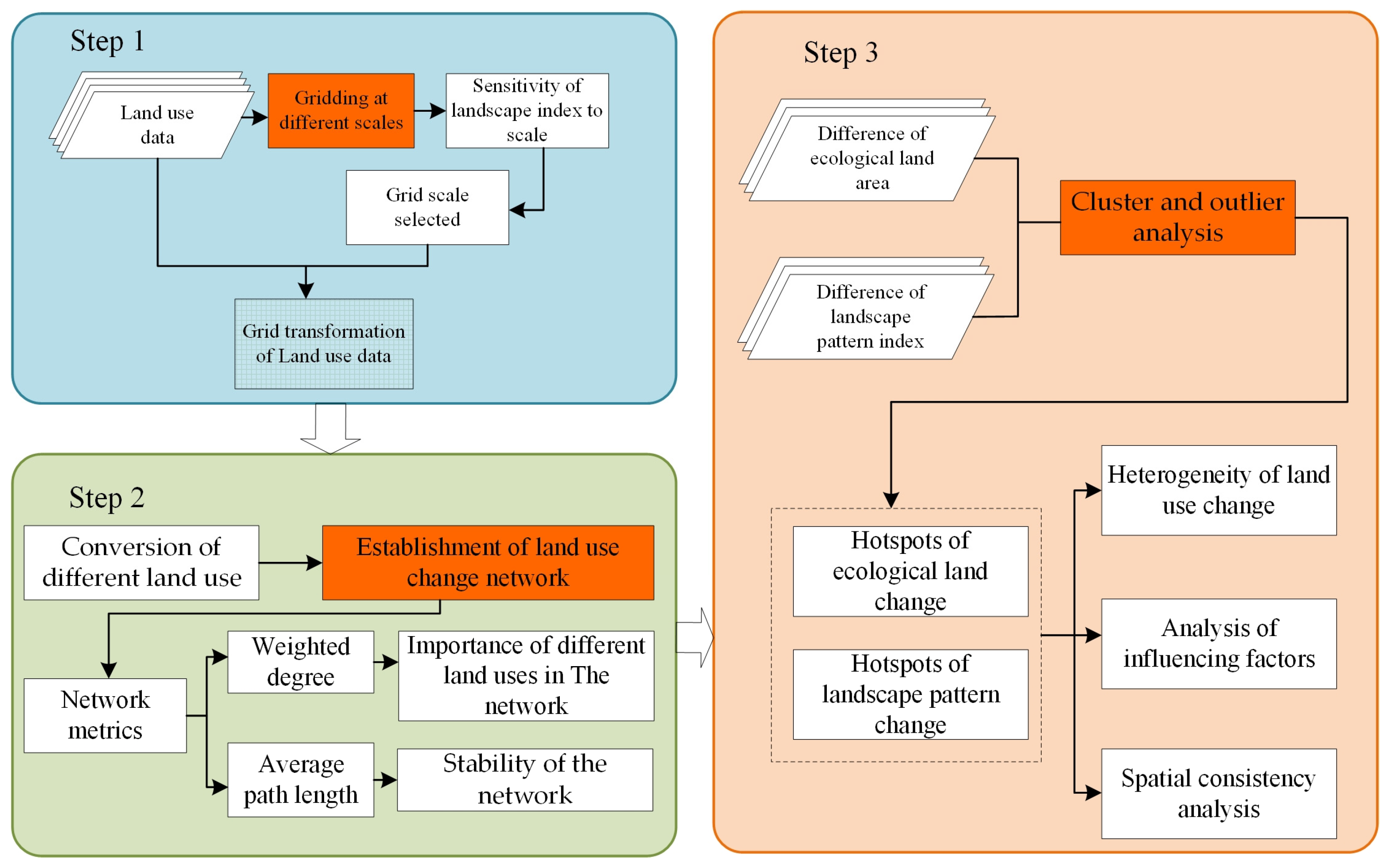
2. Materials and Methods
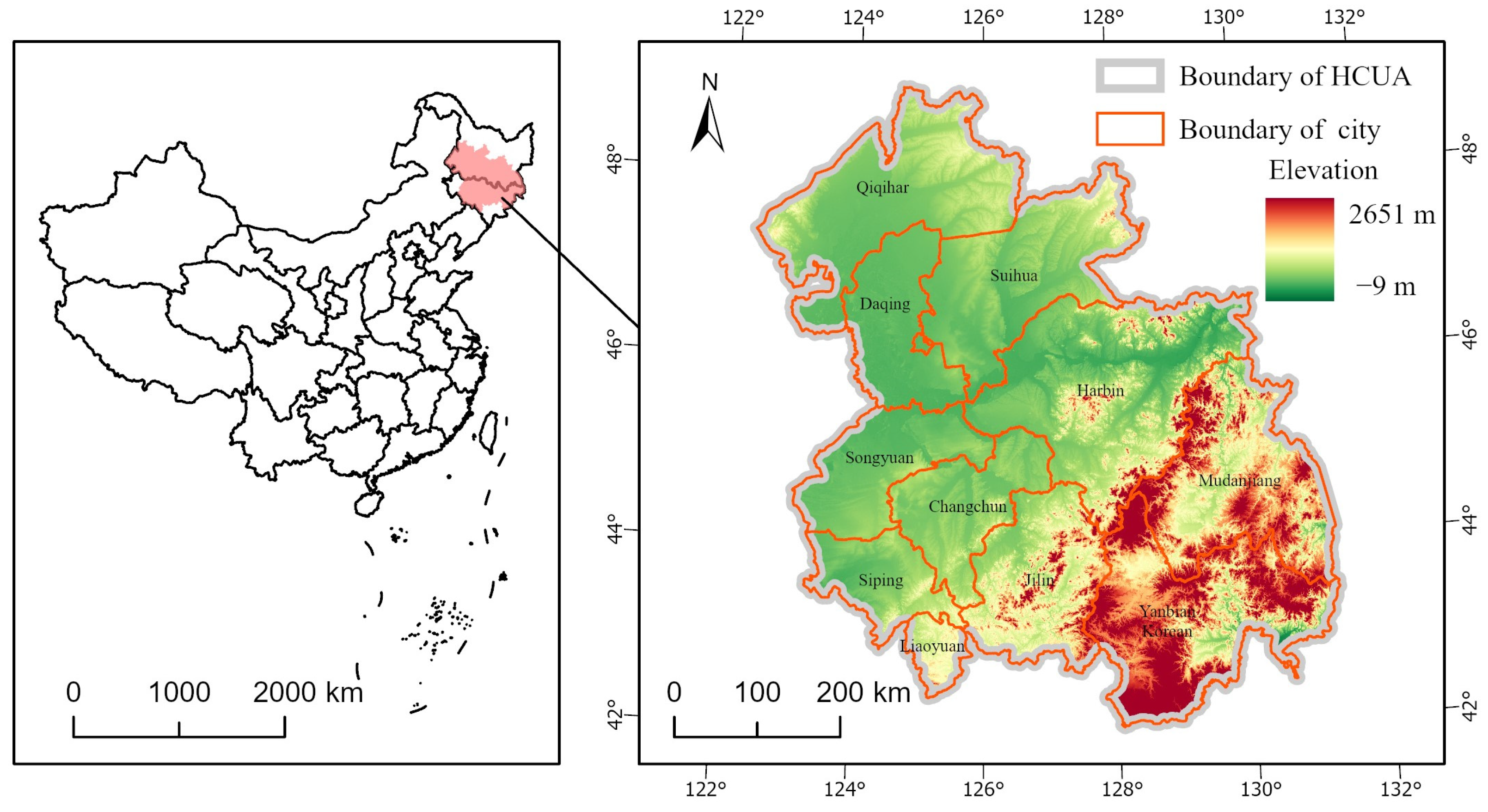
2.1. Study Area
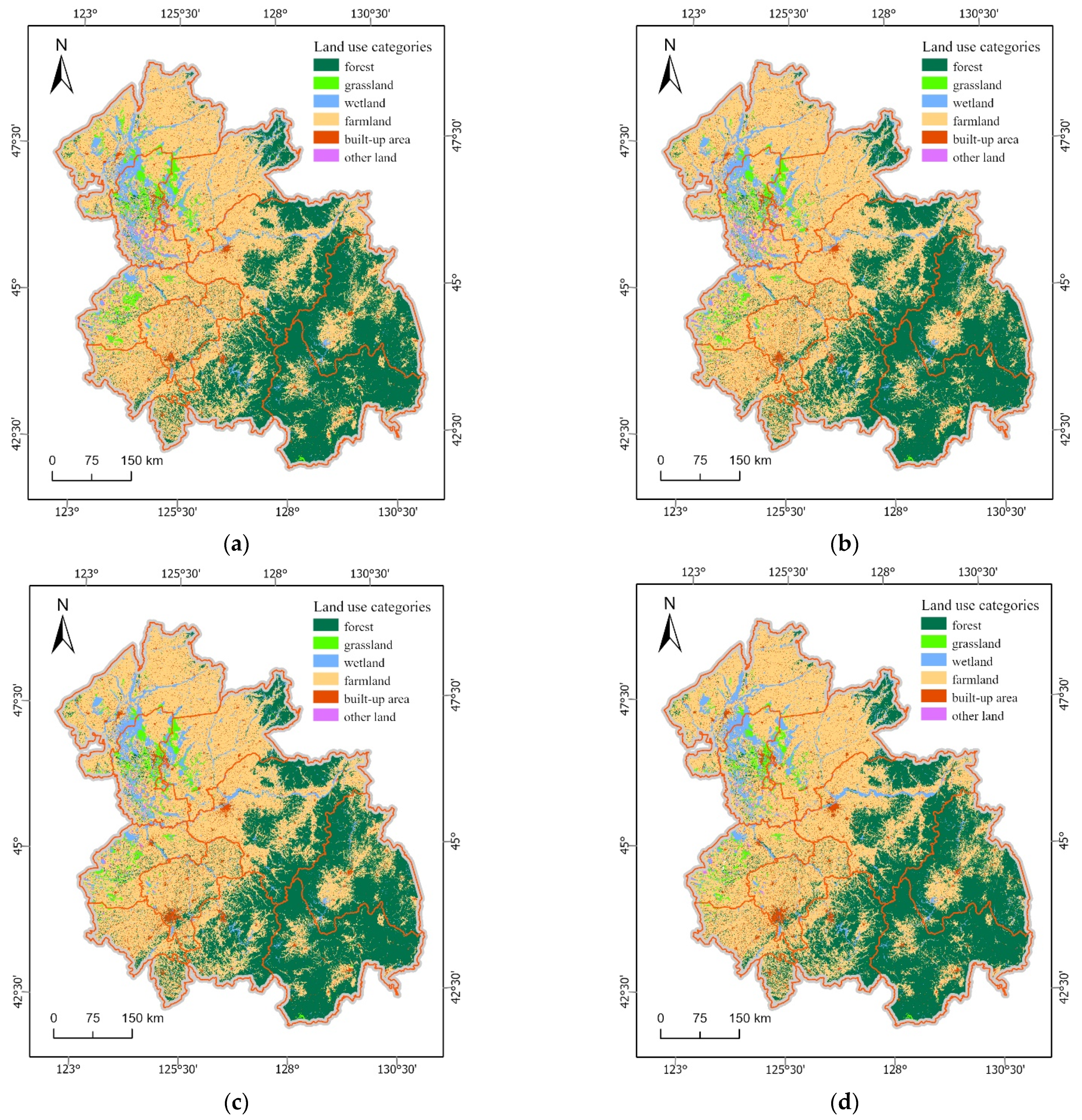
2.2. Land Use Data
2.3. Methods
2.3.1. Analysis of Land Use Conversations Based on Complex Network Model
2.3.2. Landscape Pattern Analysis
2.3.3. Hotspot Identification of Land Use Change
3. Results
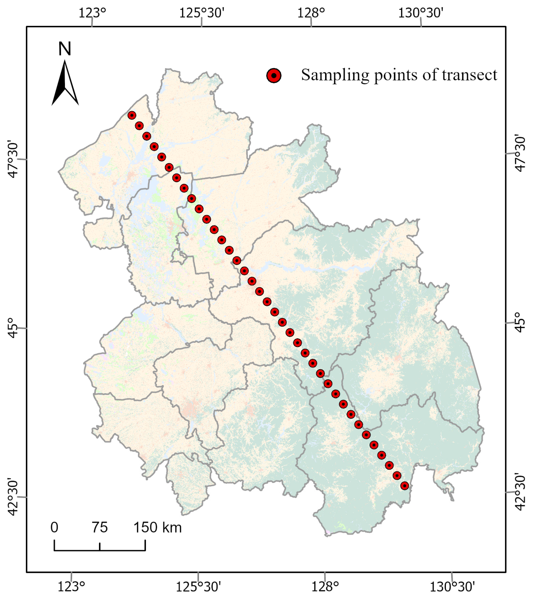
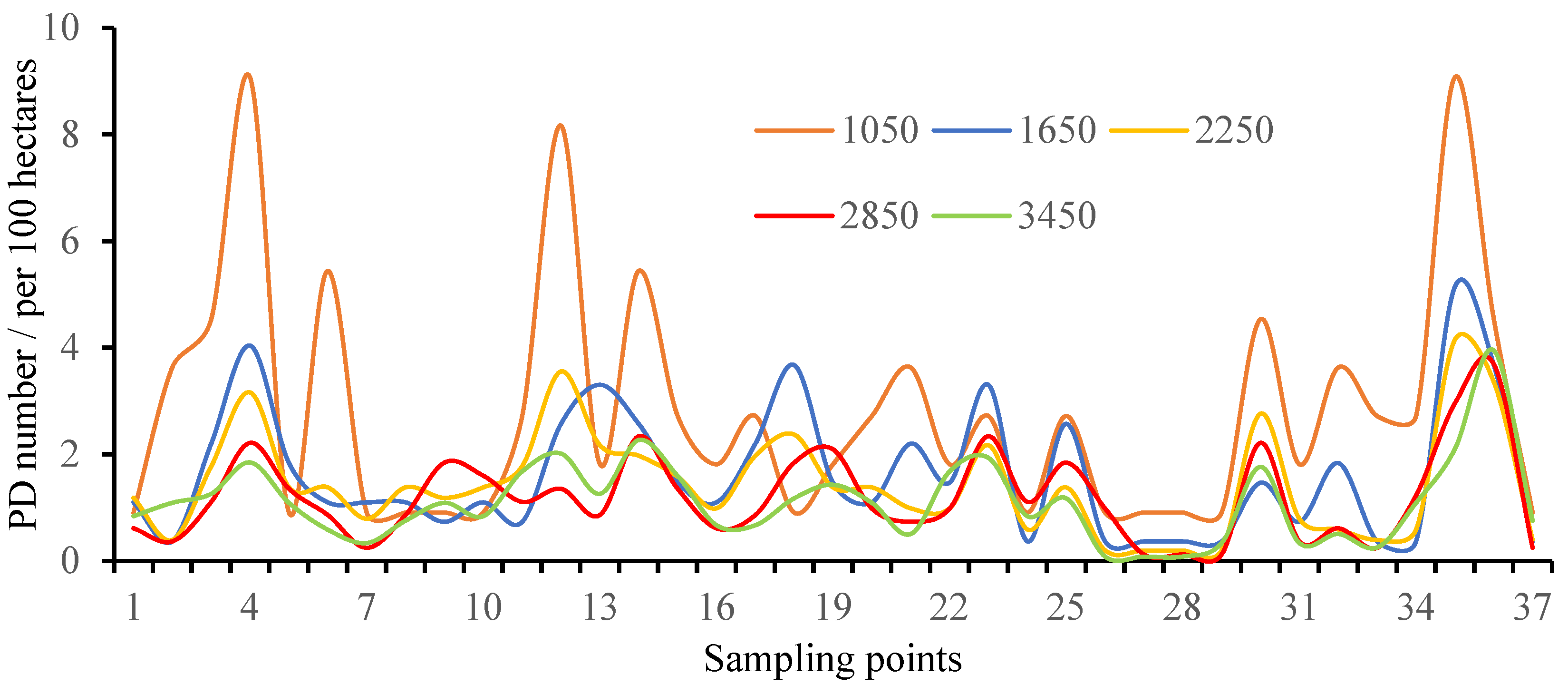
3.1. Selection of Analysis Window Size
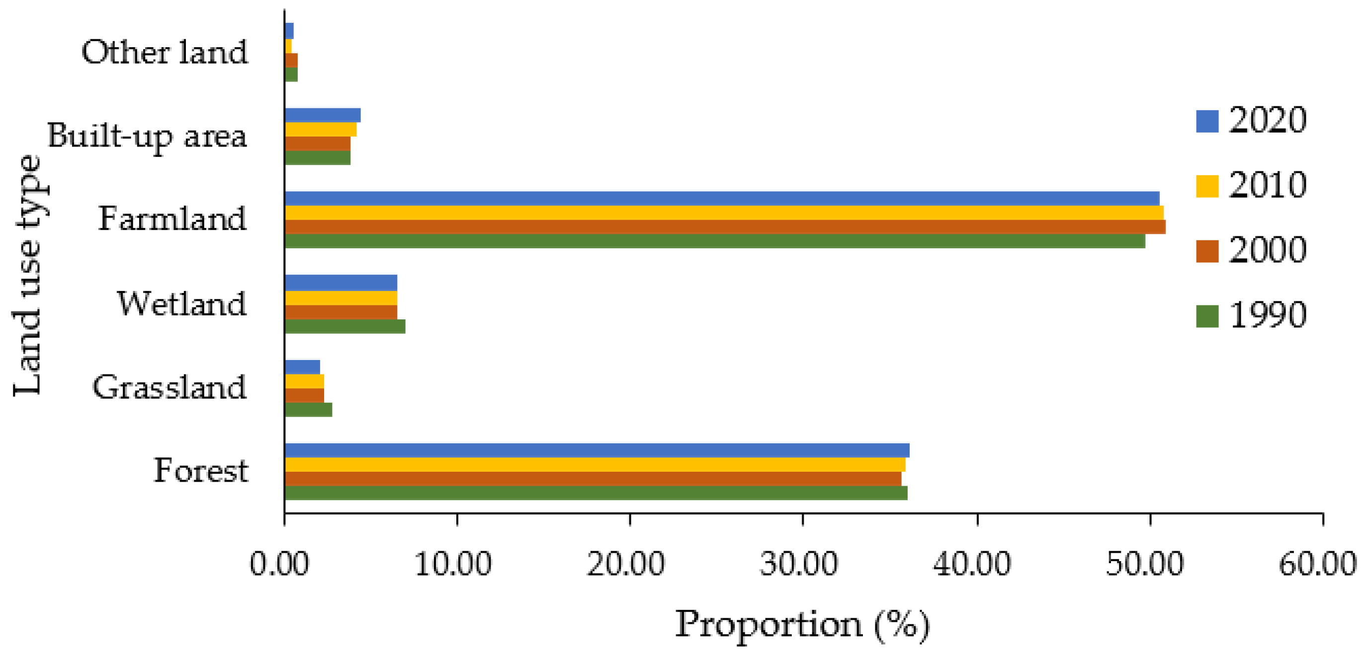
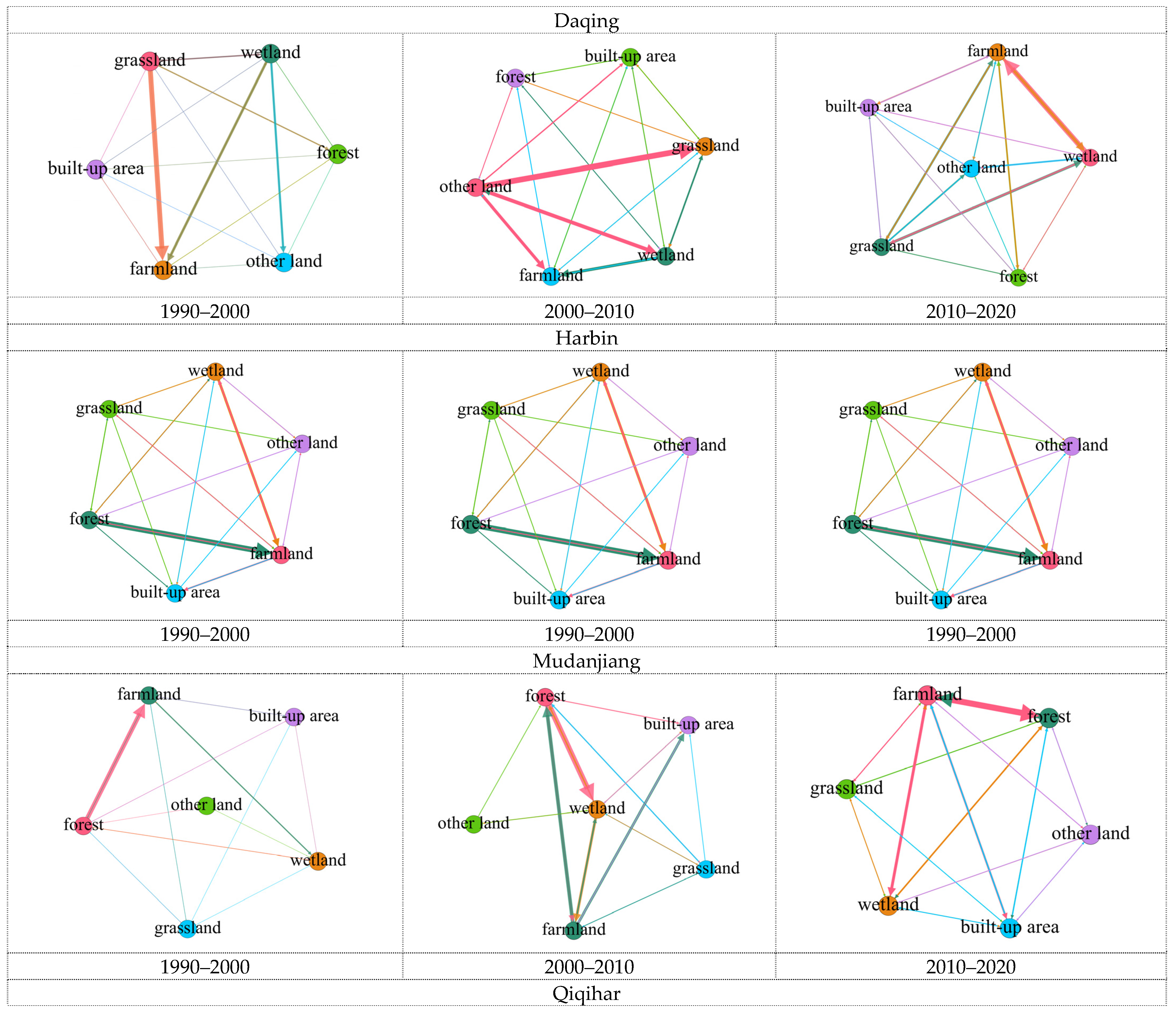
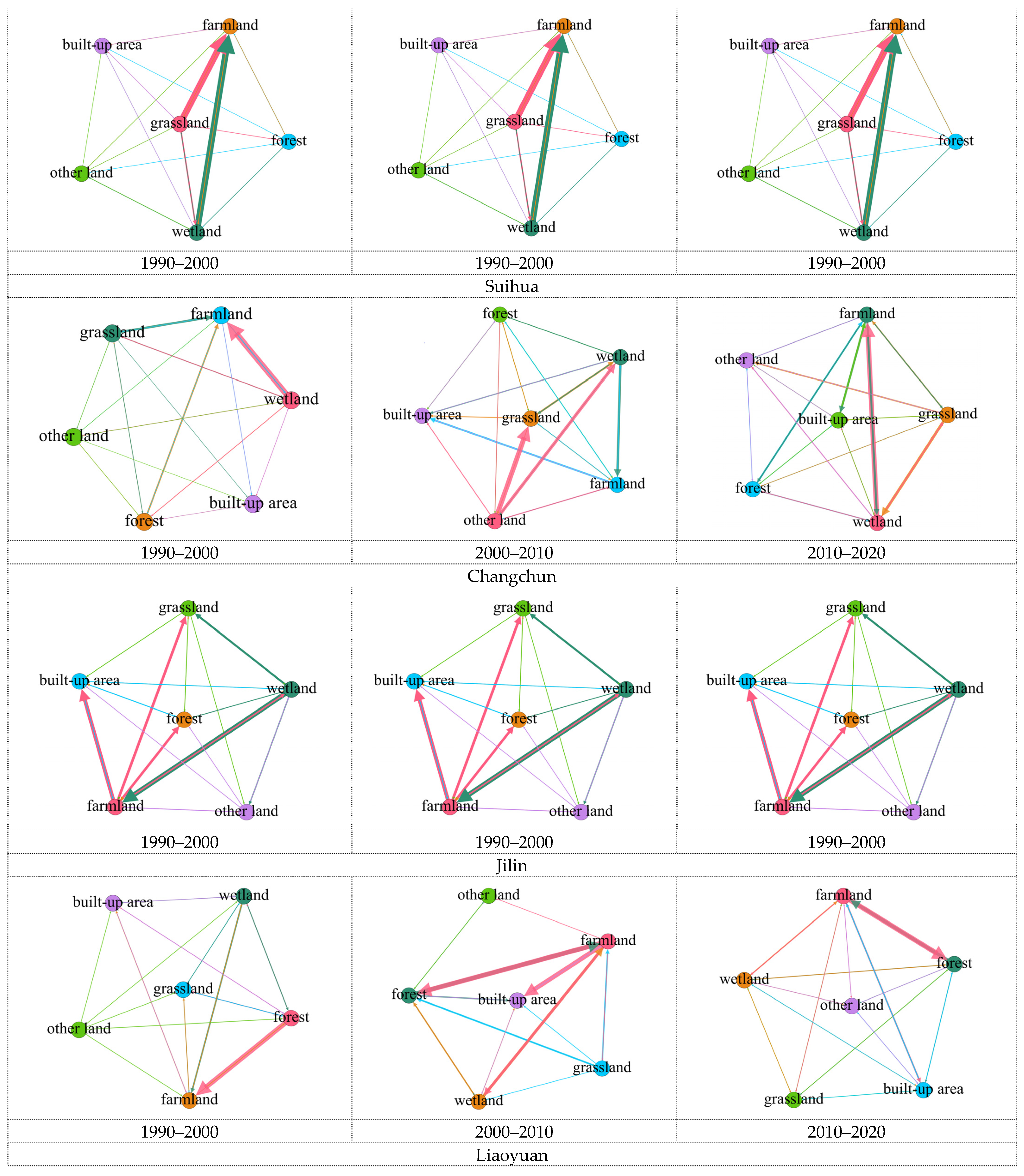
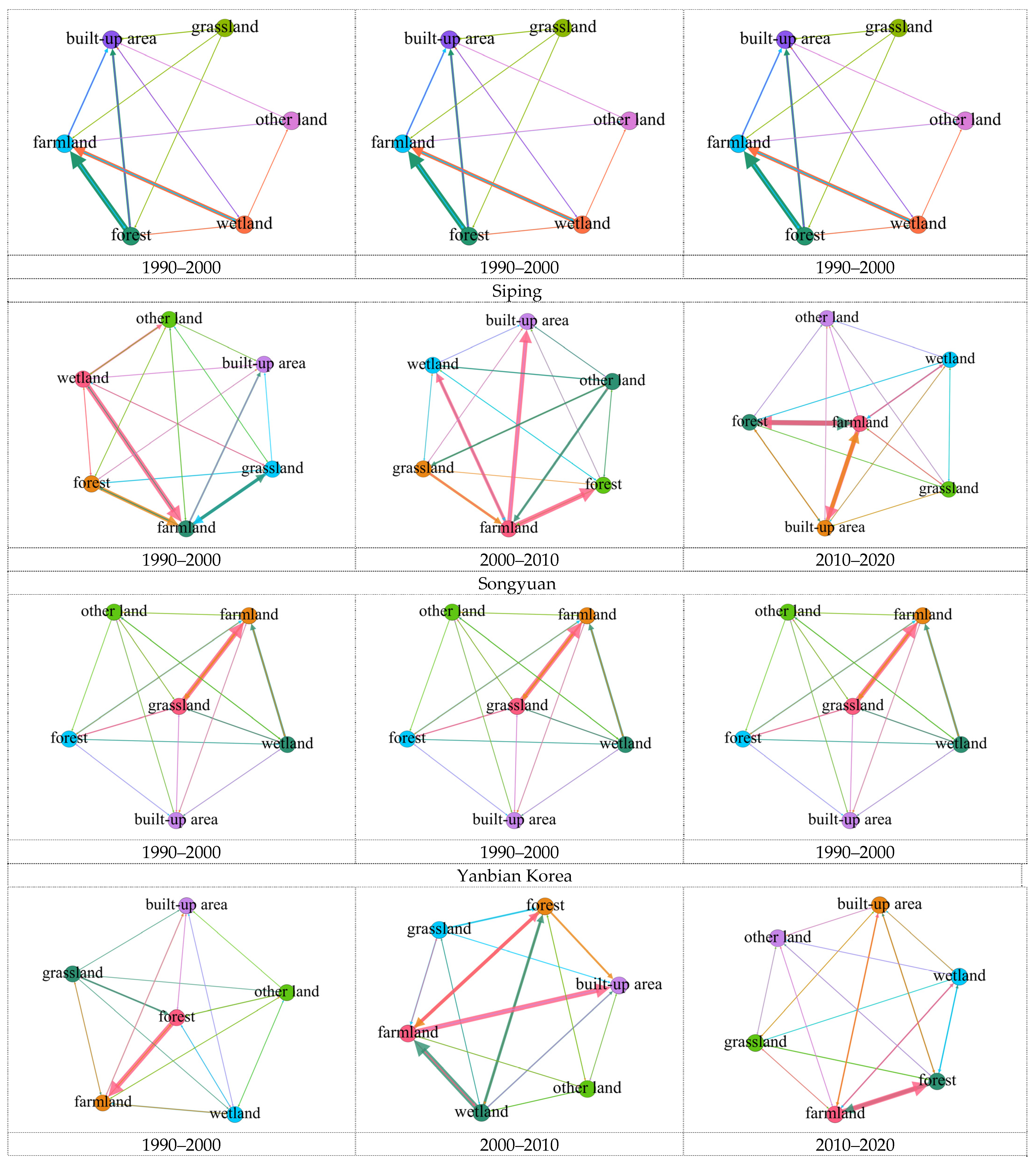
3.2. Transformation between Different Land Use Types
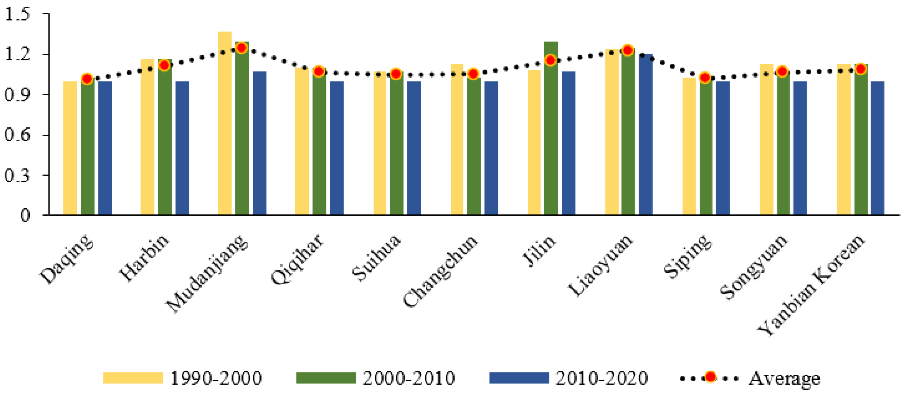
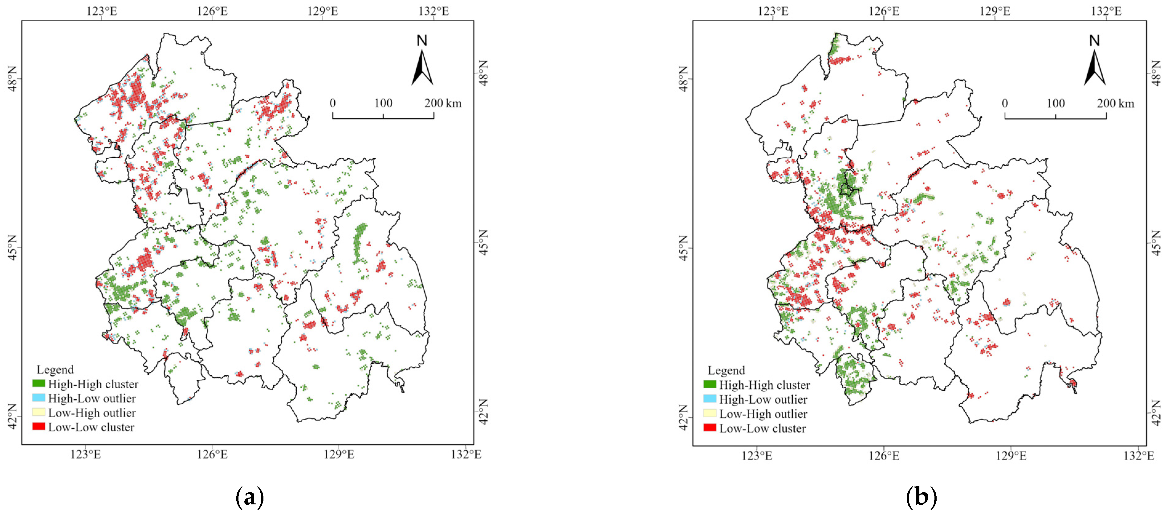
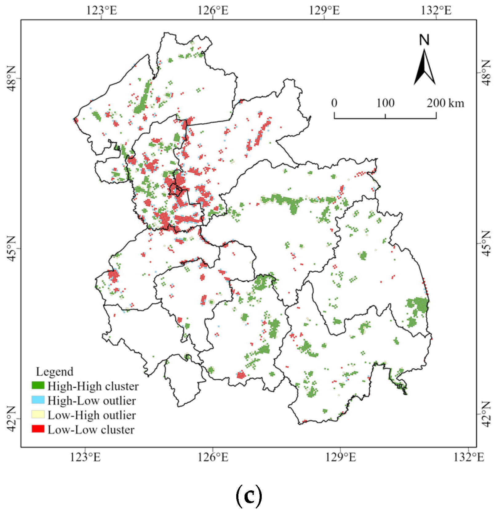
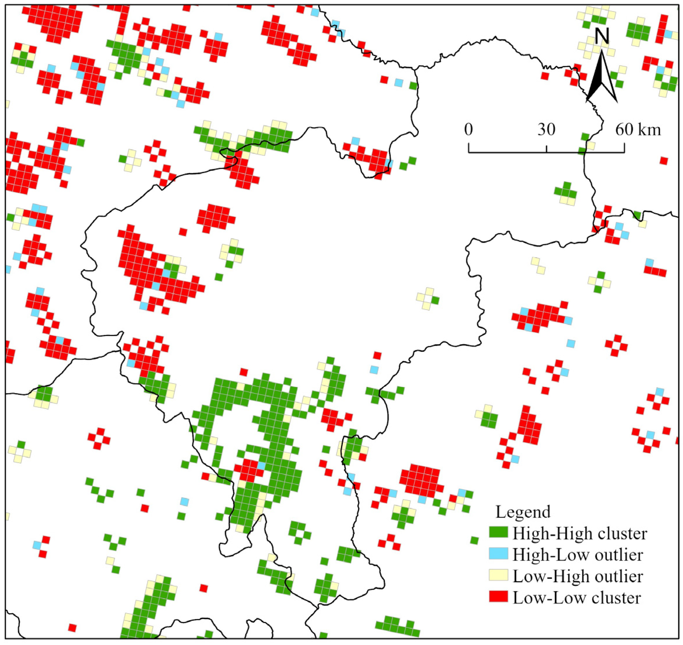
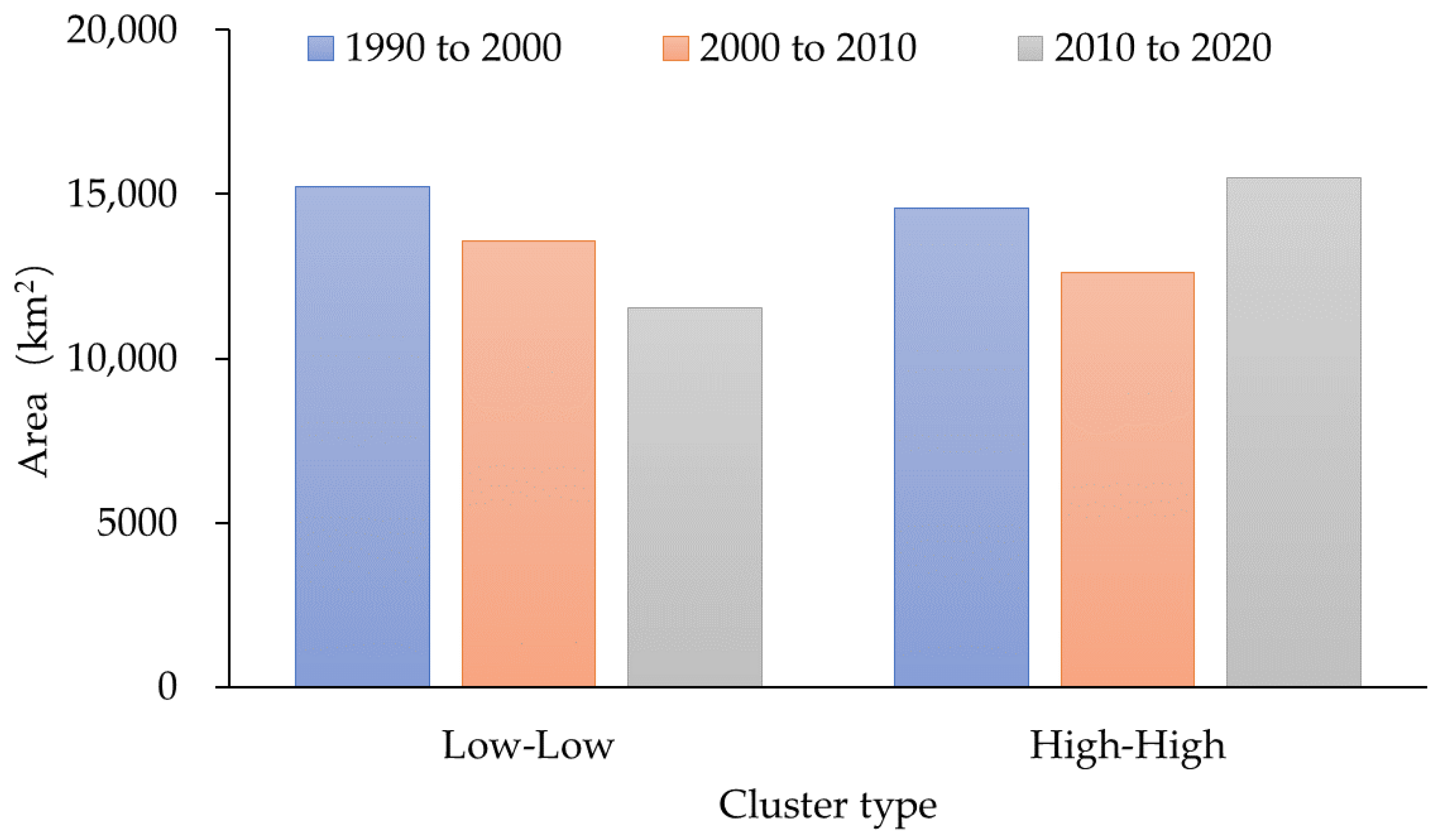
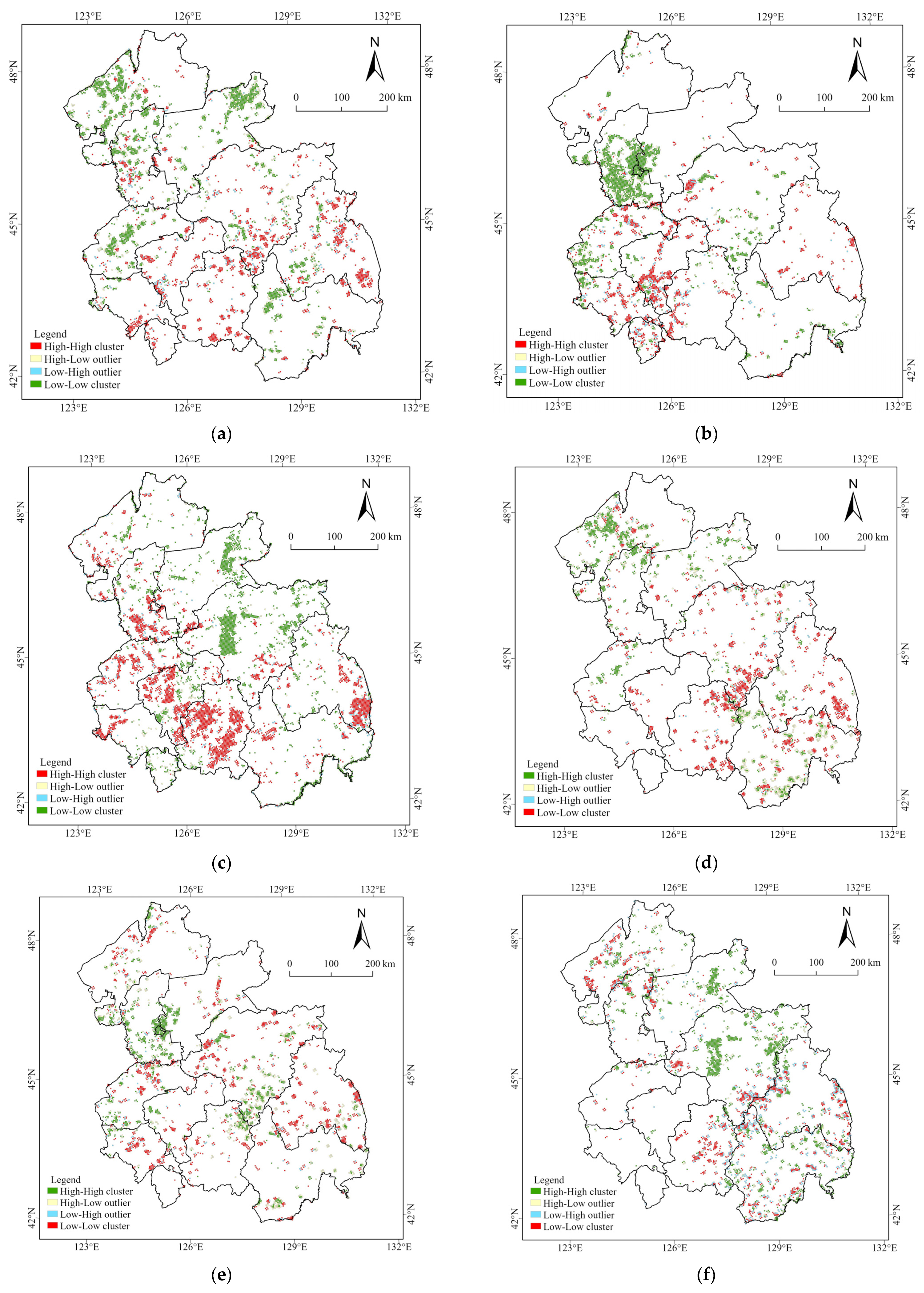
3.3. Spatiotemporal Change Hotspots of Ecological Land
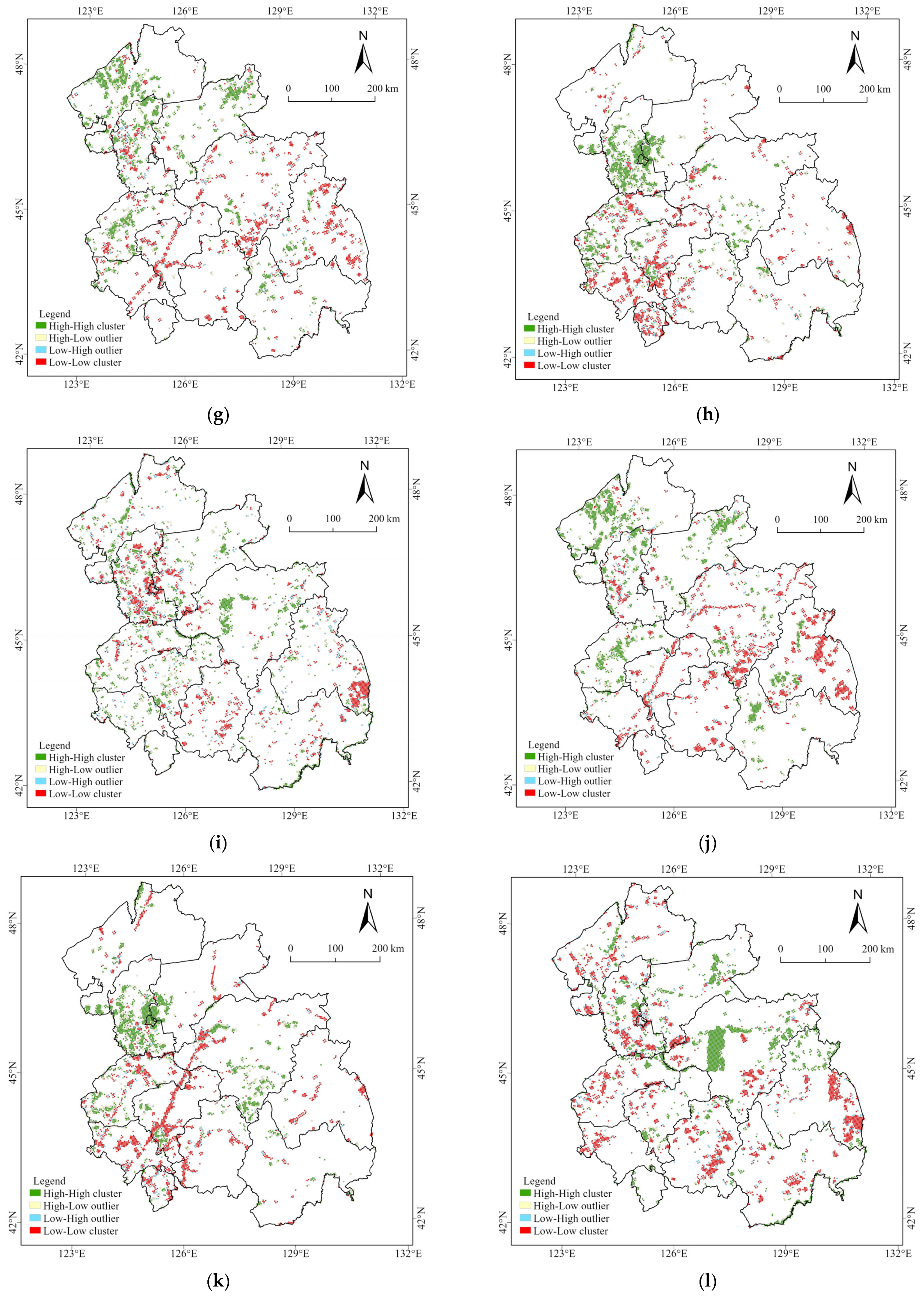
3.4. Hotspot of Spatial and Temporal Changes of Landscape Patterns
4. Discussion
4.1. Spatial Consistency of Ecological Land Use and Landscape Pattern Changes
4.2. Influencing Factors of Hotspot Distribution
4.3. Enlightenment on Balancing Urban Agglomeration Development and Ecological Protection
5. Conclusions
Author Contributions
Funding
Data Availability Statement
Acknowledgments
Conflicts of Interest
Appendix A


| Periods | City | Indicators | Land Use Categories | |||||
|---|---|---|---|---|---|---|---|---|
| Forest | Grassland | Wetland | Farmland | Built-Up Area | Other Land | |||
| 1990–2000 | Harbin | Output | 398,875.59 | 32,603.31 | 150,446.16 | 122,689.08 | 250.29 | 5494.23 |
| Input | 36,502.65 | 4583.79 | 75,858.93 | 527,696.37 | 65,126.43 | 590.49 | ||
| Daqing | Output | 1518.75 | 451,855.26 | 349,921.62 | 69,010.38 | 106.11 | 15,522.84 | |
| Input | 83,707.02 | 58,890.24 | 121,026.15 | 471,972.42 | 21,377.52 | 130,961.61 | ||
| Mudanjiang | Output | 429,867.00 | 6347.97 | 12,004.20 | 106,139.16 | 110.97 | 121.50 | |
| Input | 14,742.00 | 2387.88 | 100,013.13 | 416,973.42 | 20,126.07 | 348.30 | ||
| Qiqihar | Output | 21,895.92 | 699,136.92 | 610,521.30 | 46,300.41 | 163.62 | 1458.81 | |
| Input | 20,764.35 | 10,558.35 | 125,651.25 | 1,176,733.17 | 21,633.48 | 24,136.38 | ||
| Suihua | Output | 86,566.32 | 173,146.41 | 428,279.40 | 41,312.43 | 160.38 | 4510.08 | |
| Input | 38,788.47 | 27,387.72 | 59,954.58 | 575,188.29 | 19,030.95 | 13,625.01 | ||
| Changchun | Output | 13,735.98 | 5172.66 | 104,212.98 | 127,977.57 | 5346.81 | 2514.24 | |
| Input | 37,412.28 | 54,208.44 | 13,928.76 | 87,103.35 | 58,159.62 | 8147.79 | ||
| Jilin | Output | 158,636.07 | 5317.65 | 42,276.33 | 20,727.90 | 2736.18 | 3120.93 | |
| Input | 22,778.82 | 15,500.97 | 5665.95 | 180,357.84 | 8511.48 | 0.00 | ||
| Liaoyuan | Output | 19,321.74 | 403.38 | 10,198.71 | 4261.41 | 20.25 | 20.25 | |
| Input | 1070.82 | 0.00 | 1304.91 | 24,917.22 | 6922.26 | 10.53 | ||
| Siping | Output | 42,277.14 | 39,338.46 | 79,912.98 | 52,967.52 | 311.04 | 1193.13 | |
| Input | 13,156.83 | 34,945.83 | 2643.84 | 133,712.37 | 13,956.30 | 17,585.10 | ||
| Songyuan | Output | 157,818.78 | 40,530.78 | 23,413.05 | 30,402.54 | 177.39 | 11,442.06 | |
| Input | 55,372.41 | 1500.12 | 12,525.03 | 178,179.75 | 15,143.76 | 1063.53 | ||
| Yanbian Korean | Output | 157,818.78 | 40,530.78 | 23,413.05 | 30,402.54 | 177.39 | 11,442.06 | |
| Input | 55,372.41 | 1500.12 | 12,525.03 | 178,179.75 | 15,143.76 | 1063.53 | ||
| 2000–2010 | Harbin | Output | 48,743.37 | 28,239.84 | 133,546.32 | 434,891.43 | 3807.00 | 6578.01 |
| Input | 248,034.15 | 350.73 | 134,464.86 | 133,718.04 | 135,588.33 | 3649.86 | ||
| Daqing | Output | 1363.23 | 39,899.79 | 227,714.49 | 23,553.18 | 6196.50 | 539,485.92 | |
| Input | 19,958.40 | 291,422.61 | 181,224.54 | 229,023.45 | 52,957.80 | 63,626.31 | ||
| Mudanjiang | Output | 70,477.29 | 5101.38 | 31,207.68 | 59,534.19 | 336.96 | 886.14 | |
| Input | 43,442.73 | 421.20 | 60,269.67 | 38,673.45 | 24,731.73 | 4.86 | ||
| Qiqihar | Output | 5893.56 | 16,472.97 | 147,202.11 | 192,537.81 | 11,868.12 | 35,860.32 | |
| Input | 15,692.94 | 20,502.72 | 175,794.30 | 148,178.16 | 44,478.72 | 5188.05 | ||
| Suihua | Output | 7081.02 | 46,134.36 | 74,502.18 | 39,694.86 | 2101.14 | 175,318.83 | |
| Input | 13,957.11 | 112,572.99 | 95,649.66 | 63,547.74 | 52,866.27 | 6238.62 | ||
| Changchun | Output | 18,783.90 | 95,128.83 | 30,948.48 | 445,582.62 | 997.92 | 11,889.18 | |
| Input | 124,234.56 | 3199.50 | 120,969.45 | 100,809.36 | 247,551.39 | 6566.67 | ||
| Jilin | Output | 60,749.19 | 29,514.78 | 45,574.65 | 151,305.57 | 53.46 | 404.19 | |
| Input | 89,908.38 | 1073.25 | 31,771.44 | 95,502.24 | 69,229.89 | 116.64 | ||
| Liaoyuan | Output | 19,321.74 | 403.38 | 10,198.71 | 4261.41 | 20.25 | 20.25 | |
| Input | 1070.82 | 0.00 | 1304.91 | 24,917.22 | 6922.26 | 10.53 | ||
| Siping | Output | 12,349.26 | 40,094.19 | 19,231.02 | 223,773.84 | 427.68 | 68,438.52 | |
| Input | 98,727.66 | 21,950.19 | 60,737.04 | 96,897.06 | 84,452.22 | 1550.34 | ||
| Songyuan | Output | 26,307.18 | 268,909.47 | 287,022.69 | 156,266.82 | 106.11 | 217,318.14 | |
| Input | 54,160.65 | 224,536.05 | 133,157.52 | 422,065.08 | 77,162.22 | 44,848.89 | ||
| Yanbian Korean | Output | 45,038.43 | 16,877.97 | 73,527.75 | 75,418.29 | 26.73 | 3482.19 | |
| Input | 56,614.14 | 1996.65 | 10,321.02 | 80,874.45 | 63,238.32 | 1326.78 | ||
| 2010–2020 | Harbin | Output | 487,904.31 | 17,649.90 | 275,995.35 | 1,385,581.14 | 219,552.93 | 1967.49 |
| Input | 645,611.31 | 34,134.21 | 488,666.52 | 824,171.76 | 365,293.80 | 30,773.52 | ||
| Daqing | Output | 158,349.33 | 606,177.27 | 832,604.67 | 587,095.29 | 119,456.37 | 206,498.97 | |
| Input | 120,048.48 | 280,655.28 | 706,958.28 | 1,037,661.03 | 119,671.02 | 245,187.81 | ||
| Mudanjiang | Output | 540,994.14 | 11,369.97 | 141,312.60 | 882,242.28 | 93,474.81 | 1792.53 | |
| Input | 645,546.51 | 42,377.58 | 267,706.62 | 551,544.39 | 160,608.42 | 3402.81 | ||
| Qiqihar | Output | 133,369.74 | 170,706.69 | 461,582.55 | 1,005,417.36 | 253,187.37 | 54,764.91 | |
| Input | 141,967.89 | 95,377.50 | 727,192.89 | 793,672.83 | 300,417.66 | 20,399.85 | ||
| Suihua | Output | 206,210.61 | 485,167.32 | 692,370.99 | 494,525.25 | 167,473.98 | 15,701.85 | |
| Input | 137,474.01 | 147,444.30 | 493,724.16 | 906,909.21 | 220,008.15 | 155,890.17 | ||
| Changchun | Output | 395,369.91 | 12,215.61 | 150,450.21 | 700,795.80 | 297,738.99 | 5857.92 | |
| Input | 389,046.24 | 19,806.93 | 76,116.51 | 658,948.77 | 400,809.87 | 17,700.12 | ||
| Jilin | Output | 495,746.73 | 7545.96 | 120,447.81 | 940,107.87 | 93,818.25 | 370.98 | |
| Input | 752,515.92 | 8133.21 | 87,157.62 | 611,911.26 | 196,061.31 | 2258.28 | ||
| Liaoyuan | Output | 161,813.70 | 26.73 | 14,650.47 | 218,507.22 | 54,672.57 | 34.02 | |
| Input | 175,903.65 | 261.63 | 18,711.00 | 203,809.77 | 50,932.80 | 85.86 | ||
| Siping | Output | 247,571.64 | 19,036.62 | 49,088.43 | 461,974.59 | 189,312.39 | 11,828.43 | |
| Input | 236,855.34 | 19,593.90 | 49,020.39 | 438,991.65 | 228,142.98 | 6207.84 | ||
| Songyuan | Output | 198,905.22 | 302,651.64 | 289,905.48 | 438,248.07 | 159,694.74 | 122,298.66 | |
| Input | 215,651.16 | 184,419.18 | 167,004.99 | 620,251.02 | 155,934.72 | 168,442.74 | ||
| Yanbian Korean | Output | 443,922.12 | 37,362.87 | 103,503.42 | 699,837.57 | 113,499.63 | 4831.65 | |
| Input | 683,272.26 | 11,653.47 | 128,338.02 | 451,073.61 | 119,249.82 | 9370.08 | ||
| Data | Global Moran’s I Index | z-Score | p-Value |
|---|---|---|---|
| Change of ecological land from 1990 to 2000 | 0.49 | 139.84 | 0.00 |
| Change of ecological land from 2000 to 2010 | 0.47 | 132.72 | 0.00 |
| Change of ecological land from 2010 to 2020 | 0.57 | 160.38 | 0.00 |
| Change of PD from 1990 to 2000 | 0.00 | 3.23 | 0.00 |
| Change of PD from 2000 to 2010 | 0.24 | 70.65 | 0.00 |
| Change of PD from 2010 to 2020 | 0.01 | 2.35 | 0.02 |
| Change of AI from 1990 to 2000 | 0.22 | 67.22 | 0.00 |
| Change of AI from 2000 to 2010 | 0.39 | 109.78 | 0.00 |
| Change of AI from 2010 to 2020 | 0.22 | 62.96 | 0.00 |
| Change of MPS from 1990 to 2000 | 0.27 | 75.13 | 0.00 |
| Change of MPS from 2000 to 2010 | 0.32 | 91.51 | 0.00 |
| Change of MPS from 2010 to 2020 | 0.27 | 75.34 | 0.00 |
| Change of COHESION from 1990 to 2000 | 0.03 | 21.09 | 0.00 |
| Change of COHESION from 2000 to 2010 | 0.26 | 74.99 | 0.00 |
| Change of COHESION from 2010 to 2020 | 0.27 | 75.34 | 0.00 |


References
- Fang, C.; Yu, D. Urban agglomeration: An evolving concept of an emerging phenomenon. Landsc. Urban Plan. 2017, 162, 126–136. [Google Scholar] [CrossRef]
- Portnov, B.A.; Schwartz, M. Urban Clusters as Growth Foci. J. Reg. Sci. 2009, 49, 287–310. [Google Scholar] [CrossRef]
- Batten, D.F. Network Cities: Creative Urban Agglomerations for the 21st Century. Urban Stud. 2016, 32, 313–327. [Google Scholar] [CrossRef]
- Fang, C. Important progress and future direction of studies on China’s urban agglomerations. J. Geogr. Sci. 2015, 25, 1003–1024. [Google Scholar] [CrossRef] [Green Version]
- Chai, B.; Li, P. An ensemble method for monitoring land cover changes in urban areas using dense Landsat time series data. Isprs J. Photogramm. Remote Sens. 2023, 195, 29–42. [Google Scholar] [CrossRef]
- Asabere, S.B.; Acheampong, R.A.; Ashiagbor, G.; Beckers, S.C.; Keck, M.; Erasmi, S.; Schanze, J.; Sauer, D. Urbanization, land use transformation and spatio-environmental impacts: Analyses of trends and implications in major metropolitan regions of Ghana. Land Use Policy 2020, 96, 104707. [Google Scholar] [CrossRef]
- Esbah, H. Land use trends during rapid urbanization of the City of Aydin, Turkey. Environ. Manag. 2007, 39, 443–459. [Google Scholar] [CrossRef] [PubMed]
- Li, X.; Hu, X.; Shi, S.; Shen, L.; Luan, L.; Ma, Y. Spatiotemporal Variations and Regional Transport of Air Pollutants in Two Urban Agglomerations in Northeast China Plain. Chin. Geogr. Sci. 2019, 29, 917–933. [Google Scholar] [CrossRef] [Green Version]
- Yu, J.; Zhou, K.; Yang, S. Land use efficiency and influencing factors of urban agglomerations in China. Land Use Policy 2019, 88, 104143. [Google Scholar] [CrossRef]
- Gao, X.; Xu, Z.; Niu, F.; Long, Y. An evaluation of China’s urban agglomeration development from the spatial perspective. Spat. Stat. 2017, 21, 475–491. [Google Scholar] [CrossRef]
- Akdeniz, H.B.; Sag, N.S.; Inam, S. Analysis of land use/land cover changes and prediction of future changes with land change modeler: Case of Belek, Turkey. Environ. Monit. Assess. 2022, 195, 135. [Google Scholar] [CrossRef] [PubMed]
- Liu, S.; Li, X.; Chen, D.; Duan, Y.; Ji, H.; Zhang, L.; Chai, Q.; Hu, X. Understanding Land use/Land cover dynamics and impacts of human activities in the Mekong Delta over the last 40 years. Glob. Ecol. Conserv. 2020, 22, e00991. [Google Scholar] [CrossRef]
- De Jong, L.; De Bruin, S.; Knoop, J.; van Vliet, J. Understanding land-use change conflict: A systematic review of case studies. J. Land Use Sci. 2021, 16, 223–239. [Google Scholar] [CrossRef]
- Moon, G.; Yim, J.; Moon, N. Optimal Sampling Intensity in South Korea for a Land-Use Change Matrix Using Point Sampling. Land 2021, 10, 677. [Google Scholar] [CrossRef]
- Boccaletti, S.; Latora, V.; Moreno, Y.; Chavez, M.; Hwang, D. Complex networks: Structure and dynamics. Phys. Rep. 2006, 424, 175–308. [Google Scholar] [CrossRef]
- Yang, X.; Wen, S.; Liu, Z.; Li, C.; Huang, C. Dynamic Properties of Foreign Exchange Complex Network. Mathematics 2019, 7, 832. [Google Scholar] [CrossRef] [Green Version]
- Yue, Q.; He, J.; Liu, D. Identifying Restructuring Types of Rural Settlement Using Social Network Analysis: A Case Study of Ezhou City in Hubei Province of China. Chin. Geogr. Sci. 2021, 31, 1011–1028. [Google Scholar] [CrossRef]
- Navarro-Azorín, J.M.; Artal-Tur, A.; Ramos-Parreño, J.M. Geography and embeddedness in city networks. Spat. Econ. Ana. 2021, 17, 1–17. [Google Scholar] [CrossRef]
- Xu, C.; Pu, L.; Kong, F.; Li, B. Spatio-Temporal Change of Land Use in a Coastal Reclamation Area: A Complex Network Approach. Sustainability 2021, 13, 8690. [Google Scholar] [CrossRef]
- Bryan, B.A.; Ye, Y.; Zhang, J.e.; Connor, J.D. Land-use change impacts on ecosystem services value: Incorporating the scarcity effects of supply and demand dynamics. Ecosyst. Serv. 2018, 32, 144–157. [Google Scholar] [CrossRef]
- Yu, H.; Liu, P.; Chen, J.; Wang, H. Comparative analysis of the spatial analysis methods for hotspot identification. Accid. Anal. Prev. 2014, 66, 80–88. [Google Scholar] [CrossRef]
- Singh, M.; Yan, S. Spatial-temporal variations in deforestation hotspots in Sumatra and Kalimantan from 2001-2018. Ecol. Evol. 2021, 11, 7302–7314. [Google Scholar] [CrossRef]
- Kuemmerle, T.; Levers, C.; Erb, K.; Estel, S.; Jepsen, M.R.; Müller, D.; Plutzar, C.; Stürck, J.; Verkerk, P.J.; Verburg, P.H.; et al. Hotspots of land use change in Europe. Environ. Res. Lett. 2016, 11, 064020. [Google Scholar] [CrossRef] [Green Version]
- Duraisamy, V.; Bendapudi, R.; Jadhav, A. Identifying hotspots in land use land cover change and the drivers in a semi-arid region of India. Environ. Monit. Assess. 2018, 190, 535. [Google Scholar] [CrossRef] [PubMed] [Green Version]
- Bera, S.; Das Chatterjee, N. Mapping and monitoring of land use dynamics with their change hotspot in North 24-Parganas district, India: A geospatial- and statistical-based approach. Model. Earth Syst. Env. 2019, 5, 1529–1551. [Google Scholar] [CrossRef]
- Cao, Q.; Zhang, X.; Ma, H.; Wu, J. Review of landscape ecological risk and an assessment framework based on ecological services: ESRISK. Acta Geogr. Sin. 2018, 73, 843–855. [Google Scholar]
- Zhao, Z.; Huang, Y.; Wu, S.; Wu, Y.; Wang, Y. Study on the method of identifying the characteristics of the traffic violation behavior based on the spatial and temporal hotspot analysis approach. J. Geo-Inf. Sci. 2022, 24, 1312–1325. [Google Scholar]
- Lawson, A.B. Hotspot detection and clustering: Ways and means. Environ. Ecol. Stat. 2010, 17, 231–245. [Google Scholar] [CrossRef]
- Fahad, M.G.R.; Zech, W.C.; Nazari, R.; Karimi, M. Developing a Geospatial Framework for Severe Occupational Injuries Using Moran’s I and Getis-Ord Gi* Statistics for Southeastern United States. Nat. Hazards Rev. 2022, 23, 04022020. [Google Scholar] [CrossRef]
- Anselin, L. Local Indicators of Spatial Association—LISA. Geogr. Anal. 1995, 27, 93–115. [Google Scholar] [CrossRef]
- Alberti, M.; Marzluff, J.M. Ecological resilience in urban ecosystems: Linking urban patterns to human and ecological functions. Urban Ecosyst. 2004, 7, 241–265. [Google Scholar] [CrossRef]
- Naikoo, M.W.; Rihan, M.; Ishtiaque, M.; Shahfahad. Analyses of land use land cover (LULC) change and built-up expansion in the suburb of a metropolitan city: Spatio-temporal analysis of Delhi NCR using landsat datasets. J. Urban Manag. 2020, 9, 347–359. [Google Scholar] [CrossRef]
- Aneesha Satya, B.; Shashi, M.; Deva, P. Future land use land cover scenario simulation using open source GIS for the city of Warangal, Telangana, India. Appl. Geomat. 2020, 12, 281–290. [Google Scholar] [CrossRef]
- Shen, F.; Yang, L.; Zhang, L.; Guo, M.; Huang, H.; Zhou, C. Quantifying the direct effects of long-term dynamic land use intensity on vegetation change and its interacted effects with economic development and climate change in jiangsu, China. J. Environ. Manag. 2023, 325, 116562. [Google Scholar] [CrossRef] [PubMed]
- Lambin, E.F.; Geist, H.J.; Lepers, E. Dynamics of Land-Use and Land-Cover Change in Tropical Regions. Annu. Rev. Environ. Resour. 2003, 28, 205–241. [Google Scholar] [CrossRef] [Green Version]
- Chen, M. Economic spatial connection and evolution trend of national urban aglomeration: Take Harbin-Changchun Urban Agglomeration as an example. Econ. Geogr. 2020, 40, 99–105. [Google Scholar]
- Guo, R.; Wu, T.; Liu, M.; Huang, M.; Stendardo, L.; Zhang, Y. The Construction and Optimization of Ecological Security Pattern in the Harbin-Changchun Urban Agglomeration, China. Int. J. Environ. Res. Public Health 2019, 16, 1190. [Google Scholar] [CrossRef] [Green Version]
- Ma, X.; Chen, X.; Du, Y.; Zhu, X.; Dai, Y.; Li, X.; Zhang, R.; Wang, Y. Evaluation of Urban Spatial Resilience and Its Influencing Factors: Case Study of the Harbin–Changchun Urban Agglomeration in China. Sustainability 2022, 14, 2899. [Google Scholar] [CrossRef]
- Yu, W.; Zhou, W.; Qian, Y.; Yan, J. A new approach for land cover classification and change analysis: Integrating backdating and an object-based method. Remote Sens. Environ. 2016, 177, 37–47. [Google Scholar] [CrossRef]
- Chang, S.; Jiang, Q.; Wang, Z.; Xu, S.; Jia, M. Extraction and Spatial–Temporal Evolution of Urban Fringes: A Case Study of Changchun in Jilin Province, China. ISPRS Int. J. Geo-Inf. 2018, 7, 241. [Google Scholar] [CrossRef] [Green Version]
- Chen, L.; Ren, C.; Zhang, B.; Wang, Z.; Liu, M. Quantifying Urban Land Sprawl and its Driving Forces in Northeast China from 1990 to 2015. Sustainability 2018, 10, 188. [Google Scholar] [CrossRef] [Green Version]
- Fronczak, A.; Fronczak, P.; Holyst, J.A. Average path length in random networks. Phys. Rev. E 2004, 70, 056110. [Google Scholar] [CrossRef] [PubMed] [Green Version]
- Kwapień, J.; Drożdż, S. Physical approach to complex systems. Phys. Rep. 2012, 515, 115–226. [Google Scholar] [CrossRef]
- Jianguo, W. Landscape Ecology Pattern, Process, Scale and Hierarchy; Higher Education Press: Beijing, China, 2000. [Google Scholar]
- Wu, J.; Shen, W.; Sun, W.; Tueller, P.T. Empirical patterns of the effects of changing scale on landscape metrics. Landscape Ecol. 2002, 17, 761–782. [Google Scholar] [CrossRef]
- Plexida, S.G.; Sfougaris, A.I.; Ispikoudis, I.P.; Papanastasis, V.P. Selecting landscape metrics as indicators of spatial heterogeneity—A comparison among Greek landscapes. Int. J. Appl. Earth Obs. 2014, 26, 26–35. [Google Scholar] [CrossRef]
- He, H.S.; DeZonia, B.E.; Mladenoff, D.J. An aggregation index (AI) to quantify spatial patterns of landscapes. Landscape Ecol. 2000, 15, 591–601. [Google Scholar] [CrossRef]
- Gao, Y.; Cheng, J.; Meng, H.; Liu, Y. Measuring spatio-temporal autocorrelation in time series data of collective human mobility. Geo-spat. Inf. Sci. 2019, 22, 166–173. [Google Scholar] [CrossRef] [Green Version]
- Ghaemi, Z.; Farnaghi, M. Event detection from geotagged tweets considering spatial autocorrelation and heterogeneity. J. Spat. Sci. 2021, 66, 1–19. [Google Scholar] [CrossRef]
- Luo, J.; Zhou, T.; Du, P.; Xu, Z. Spatial-temporal variations of natural suitability of human settlement environment in the Three Gorges Reservoir Area—A case study in Fengjie County, China. Front. Earth Sci. 2018, 13, 1–17. [Google Scholar] [CrossRef]
- Grossman, G.M.; Krueger, A.B. Economic growth and the environment. Q. J. Econ. 1995, 110, 353–377. [Google Scholar] [CrossRef] [Green Version]
- Dadashpoor, H.; Azizi, P.; Moghadasi, M. Land use change, urbanization, and change in landscape pattern in a metropolitan area. Sci. Total Environ. 2019, 655, 707–719. [Google Scholar] [CrossRef] [PubMed]
- Yang, J.; Zeng, C.; Cheng, Y. Spatial influence of ecological networks on land use intensity. Sci. Total Environ. 2020, 717, 137151. [Google Scholar] [CrossRef] [PubMed]
- Zhang, W.; Chang, W.J.; Zhu, Z.C.; Hui, Z. Landscape ecological risk assessment of Chinese coastal cities based on land use change. Appl. Geogr. 2020, 117, 102174. [Google Scholar] [CrossRef]
- Mao, D.; He, X.; Wang, Z.; Tian, Y.; Xiang, H.; Yu, H.; Man, W.; Jia, M.; Ren, C.; Zheng, H. Diverse policies leading to contrasting impacts on land cover and ecosystem services in Northeast China. J. Clean. Prod. 2019, 240, 117961. [Google Scholar] [CrossRef]
- Guyer, J.I.; Lambin, E.F.; Cliggett, L.; Walker, P.; Amanor, K.; Bassett, T.; Colson, E.; Hay, R.; Homewood, K.; Linares, O.; et al. Temporal Heterogeneity in the Study of African Land Use. Hum. Ecol. 2007, 35, 3–17. [Google Scholar] [CrossRef]
- Bryan, B.A. Incentives, land use, and ecosystem services: Synthesizing complex linkages. Environ. Sci. Policy 2013, 27, 124–134. [Google Scholar] [CrossRef] [Green Version]
- Zhou, Y.; Li, X.; Liu, Y. Land use change and driving factors in rural China during the period 1995–2015. Land Use Policy 2020, 99, 105048. [Google Scholar] [CrossRef]
- Xiao, J.; Shen, Y.; Ge, J.; Tateishi, R.; Tang, C.; Liang, Y.; Huang, Z. Evaluating urban expansion and land use change in Shijiazhuang, China, by using GIS and remote sensing. Landscape Urban Plan. 2006, 75, 69–80. [Google Scholar] [CrossRef]
- Punzo, G.; Castellano, R.; Bruno, E. Using geographically weighted regressions to explore spatial heterogeneity of land use influencing factors in Campania (Southern Italy). Land Use Policy 2022, 112, 105853. [Google Scholar] [CrossRef]
- Colding, J. ‘Ecological land-use complementation’ for building resilience in urban ecosystems. Landscape Urban Plan. 2007, 81, 46–55. [Google Scholar] [CrossRef]


| Landscape Pattern | Index | Abbreviation | Definition | Description |
|---|---|---|---|---|
| Fragmentation | Patch density [45] | PD | N is the number of patches, and a is the total area of patches. | |
| Mean patch size [45] | MPS | A is the total area of patches, and N is the total number of patches. | ||
| Connectivity | Patch cohesion Index [46] | COHESION | The smaller the value is, the more dispersed the patches are in a specific range. | |
| Aggregation index [47] | AI | The aggregation index describes the aggregation degree of patches in the landscape and reflects the dispersion of landscape elements. The smaller the value is, the higher the dispersion degree of patches is. |
Disclaimer/Publisher’s Note: The statements, opinions and data contained in all publications are solely those of the individual author(s) and contributor(s) and not of MDPI and/or the editor(s). MDPI and/or the editor(s) disclaim responsibility for any injury to people or property resulting from any ideas, methods, instructions or products referred to in the content. |
© 2023 by the authors. Licensee MDPI, Basel, Switzerland. This article is an open access article distributed under the terms and conditions of the Creative Commons Attribution (CC BY) license (https://creativecommons.org/licenses/by/4.0/).
Share and Cite
Chang, S.; Zhao, J.; Jia, M.; Mao, D.; Wang, Z.; Hou, B. Land Use Change and Hotspot Identification in Harbin–Changchun Urban Agglomeration in China from 1990 to 2020. ISPRS Int. J. Geo-Inf. 2023, 12, 80. https://doi.org/10.3390/ijgi12020080
Chang S, Zhao J, Jia M, Mao D, Wang Z, Hou B. Land Use Change and Hotspot Identification in Harbin–Changchun Urban Agglomeration in China from 1990 to 2020. ISPRS International Journal of Geo-Information. 2023; 12(2):80. https://doi.org/10.3390/ijgi12020080
Chicago/Turabian StyleChang, Shouzhi, Jian Zhao, Mingming Jia, Dehua Mao, Zongming Wang, and Boyu Hou. 2023. "Land Use Change and Hotspot Identification in Harbin–Changchun Urban Agglomeration in China from 1990 to 2020" ISPRS International Journal of Geo-Information 12, no. 2: 80. https://doi.org/10.3390/ijgi12020080