


Spatial Application of Southern U.S. Pine Water Yield for Prioritizing Forest Management Activities
 , and
, and
Abstract
:1. Introduction
2. Materials and Methods
2.1. Study Area
2.2. Stand-Level Water Yield Model
2.3. Geospatial Data
2.3.1. Pine Basal Area
2.3.2. Depth to Water Table
2.3.3. Aridity Index
2.4. Spatial Water Yield Estimation Workflow
2.5. Timber Thinning and Climate Scenarios
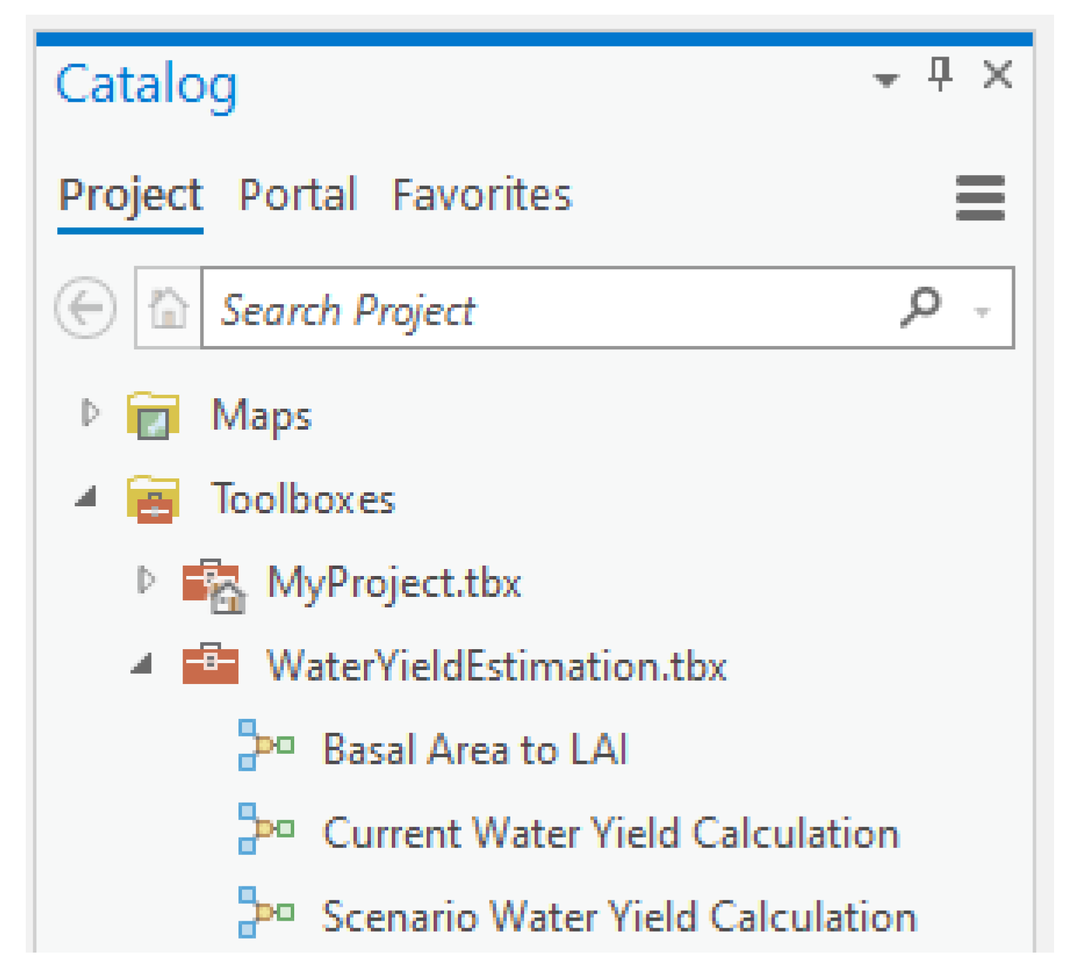
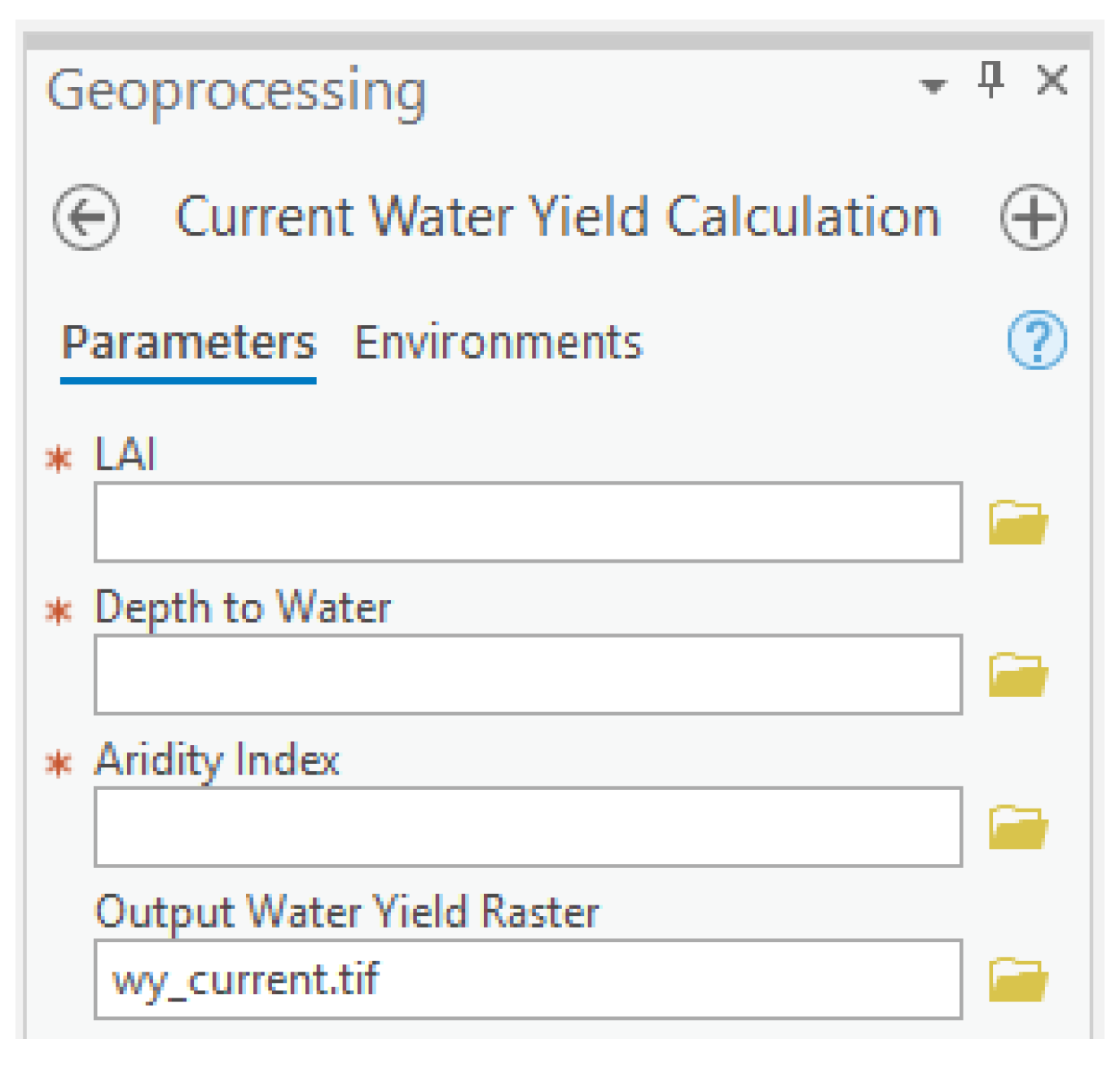
2.6. Workflow Automation Tools
3. Results
4. Discussion
4.1. Applications of WY in Forest Management
4.2. Model Limitations and Future Research
5. Conclusions
Author Contributions
Funding
Data Availability Statement
Acknowledgments
Conflicts of Interest
Appendix A


Appendix B
References
- Recknagel, F. Ecological Informatics: A discipline in the making. Ecol. Inform. 2011, 6, 1–3. [Google Scholar] [CrossRef]
- Sonti, S.H. Application of Geographic Information System (GIS) in Forest Management. J. Geogr. Nat. Disasters 2015, 5, 1000145. [Google Scholar]
- Segura, M.; Ray, D.; Maroto, C. Decision support systems for forest management: A comparative analysis and assessment. Comput. Electron. Agric. 2014, 101, 55–67. [Google Scholar] [CrossRef]
- Gholz, H.L.; Clark, K.L. Energy exchange across a chronosequence of slash pine forests in Florida. Agric. For. Meteorol. 2002, 112, 87–102. [Google Scholar] [CrossRef]
- Acharya, S.; Kaplan, D.A.; McLaughlin, D.L.; Cohen, M.J. In-Situ Quantification and Prediction of Water Yield From Southern US Pine Forests. Water Resour. Res. 2022, 58, s2021WR031020. [Google Scholar] [CrossRef]
- Grier, C.C.; Running, S.W. Leaf Area of Mature Northwestern Coniferous Forests: Relation to Stie Water Balance. Ecology 1977, 58, 893–899. [Google Scholar] [CrossRef] [Green Version]
- Sun, G.; Caldwell, P.V.; McNulty, S.G. Modeling the potential role of forest thinning in maintaining water supplies under a changing climate across the conterminous United States. Hydrol. Process. 2015, 29, 5016–5030. [Google Scholar] [CrossRef]
- McLaughlin, D.L.; Kaplan, D.A.; Cohen, M.J. Managing Forests for Increased Regional Water Yield in the Southeastern U.S. Coastal Plain. J. Am. Water Resour. Assoc. 2013, 49, 953–965. [Google Scholar] [CrossRef]
- Liu, N.; Caldwell, P.V.; Dobbs, G.R.; Miniat, C.F.; Bolstad, P.V.; Nelson, S.A.C.; Sun, G. Forested lands dominate drinking water supply in the conterminous United States. Environ. Res. Lett. 2021, 16, 084008. [Google Scholar] [CrossRef]
- Bruijnzeel, L.A. Hydrological functions of tropical forests: Not seeing the soil for the trees? Agric. Ecosyst. Environ. 2004, 104, 185–228. [Google Scholar] [CrossRef]
- Ahmed, M.A.A.; Abd-Elrahman, A.; Escobedo, F.J.; Cropper, W.P., Jr.; Martin, T.A.; Timilsina, N. Spatially-explicit modeling of multi-scale drivers of aboveground forest biomass and water yield in watersheds of the Southeastern United States. J. Environ. Manag. 2017, 199, 158–171. [Google Scholar] [CrossRef] [PubMed]
- Brown, T.C.; Hobbins, M.T.; Ramierez, J.A. Spatial Distribution of Water Supply in the Coterminous United States. J. Am. Water Resour. Assoc. 2008, 44, 1474–1487. [Google Scholar] [CrossRef]
- Caldwell, P.V.; Muldoon, C.; Miniat, C.F.; Cohen, E.; Krieger, S.; Sun, G.; McNulty, S.; Bolstad, P.V. Quantifying the Role of National Forest System Lands in Providing Surface Drinking Water Supply for the Southern United States; USDA For. Serv. South. Res. Stn., Gen. Tech. Rep. SRS-197; US Department of Agriculture Forest Service, Southern Research Station: Asheville, NC, USA, 2014; 135p. [CrossRef]
- Lockaby, G.; Nagy, C.; Vose, J.M.; Ford, C.R.; Sun, G.; McNulty, S.; Caldwell, P.; Cohen, E.; Myers, J.M. Forests and Water. In The Southern Forest Futures Project; Wear, D.N., Greis, J.G., Eds.; Technical Report; Gen. Tech. Rep. SRS-178; USDA Forest Service Southern Research Station: Asheville, NC, USA, 2013; 542p. [Google Scholar] [CrossRef]
- Zhang, M.; Liu, N.; Harper, R.; Li, Q.; Liu, K.; Wei, X.; Ning, D.; Hou, Y.; Liu, S. A global review on hydrological responses to forest change across multiple spatial scales: Importance of scale, climate, forest type and hydrological regime. J. Hydrol. 2017, 546, 44–59. [Google Scholar] [CrossRef] [Green Version]
- Hallema, D.W.; Sun, G.; Caldwell, P.V.; Norman, S.P.; Cohen, E.C.; Liu, Y.; Bladon, K.D.; McNulty, S.G. Burned forests impact water supplies. Nat. Commun. 2018, 9, 1307. [Google Scholar] [CrossRef] [PubMed] [Green Version]
- Cohen, M.; McLaughlin, D.; Kaplan, D.; Acharya, S. Managing Forests for Increased Regional Water Availability. FDACS Contract No. 20834 Final Report. 2018. Available online: https://www.fdacs.gov/content/download/76293/file/20834_Del_7.pdf (accessed on 13 October 2021).
- Goeking, S.A.; Tarboton, D.G. Forests and Water Yield: A Synthesis of Disturbance Effects on Streamflow and Snowpack in Western Coniferous Forests. J. For. 2020, 118, 172–192. [Google Scholar] [CrossRef] [Green Version]
- Powell, T.L.; Starr, G.; Clark, K.L.; Martin, T.A.; Gholz, H.L. Ecosystem and understory water and energy exchange for a mature, naturally regenerated pine flatwoods forest in north Florida. Can. J. For. Res. 2005, 35, 1568–1580. [Google Scholar] [CrossRef]
- Bracho, R.; Powell, T.L.; Dore, S.; Li, J.; Hinkle, R.; Drake, B.G. Environmental and biological controls on water and energy exchange in Florida scrub oak and pine flatwoods ecosystems. J. Geophys. Res. 2008, 113, G02004. [Google Scholar] [CrossRef] [Green Version]
- Susaeta, A.; Alavalapati, J. Forest Ownership, Management, and Water Production in Longleaf Pine Forests: A Stochastic Frontier Analysis. For. Sci. 2021, 67, 145–155. [Google Scholar] [CrossRef]
- Vose, J.M.; Peterson, D.L.; Patel-Weynand, T. Effects of Climatic Variability and Change on Forest Ecosystems: A Comprehensive Science Synthesis for the U.S. Forest Sector; USDA For. Serv. Pac. Northwest Res. Stn. Gen. Tech. Rep. PNW-GTR-870; USDA Forest Service Southern Research Station: Asheville, NC, USA, 2012; 282p. [CrossRef]
- Amatya, D.M.; Sun, G.; Rossi, C.G.; Ssegane, H.S.; Nettles, J.E.; Panda, S. Forests, Land Use Change, and Water. In Impact of Climate Change on Water Resources in Agriculture, 1st ed.; Zolin, C.A., Rodrigues, A.R., Eds.; CRC Press: Boca Raton, FL, USA, 2015. [Google Scholar] [CrossRef]
- Joyce, L.A.; Running, S.W.; Breshears, D.D.; Dale, V.H.; Malmsheimer, R.W.; Sampson, R.N.; Sohngen, B.; Woodall, C.W. Forests [Chapter 7]. In Climate Change Impacts in the United States: The Third National Climate Assessment, 1st ed.; Melillo, J.M., Richmond, T.C., Yohe, G.W., Eds.; Global Change Research Program: Washington, DC, USA, 2014; pp. 175–194. [Google Scholar]
- De Steven, D.; Toner, M.M. Vegetation of Upper Coastal Plain depression wetlands: Environmental templates and wetland dynamics within a landscape framework. Wetlands 2004, 24, 23–42. [Google Scholar] [CrossRef] [Green Version]
- Liu, G.; Schwartz, F.W. An integrated observational and model-based analysis of the hydrologic response of prairie pothole systems to a variability in climate. Water Resour. Res. 2010, 47, W02504. [Google Scholar] [CrossRef]
- Grant, G.E.; Tague, C.L.; Allen, C.D. Watering the forest for the trees: An emerging priority for managing water in forest landscapes. Front. Ecol. Environ. 2013, 11, 314–321. [Google Scholar] [CrossRef] [PubMed] [Green Version]
- Almeida, B.; Cabral, P. Water Yield Modelling, Sensitivity Analysis and Validation: A Study for Portugal. ISPRS Int. J. Geo-Inf. 2021, 10, 494. [Google Scholar] [CrossRef]
- Asurza-Véliz, F.A.; Lavado-Casimiro, W.S. Regional Parameter Estimation of the SWAT Model: Methodology and Application to River Basins in the Peruvian Pacific Drainage. Water 2020, 12, 3198. [Google Scholar] [CrossRef]
- Brown, T.C.; Froemke, P.; Mahat, W.; Ramirez, J. Mean Annual Renewable Water Supply of the Contiguous United States; Briefing paper; Rocky Mountain Research Station: Fort Collins, CO, USA, 2016; 55p. Available online: https://www.fs.usda.gov/rmrs/sites/default/files/documents/source%20of%20water%20supply%2C%20web%203.pdf (accessed on 22 September 2022).
- Ayivi, F.; Jha, M.K. Estimation of water balance and water yield in the Reedy Fork-Buffalo Creek Watershed in North Carolina using SWAT. Int. Soil Water Conserv. Res. 2018, 6, 203–213. [Google Scholar] [CrossRef]
- Cademus, R.; Escobedo, F.J.; McLaughlin, D.; Abd-Elrahman, A. Analyzing Trade-Offs, Synergies, and Drivers among Timber Production, Carbon Sequestration, and Water Yield in Pinus elliotii Forests in Southeastern USA. Forests 2014, 5, 1409–1431. [Google Scholar] [CrossRef] [Green Version]
- St. Peter, J.; Drake, J.; Medley, P.; Ibeanusi, V. Forest Structural Estimates Derived Using a Practical, Open-source Lidar-Processing Workflow. Remote Sens. 2021, 13, 4763. [Google Scholar] [CrossRef]
- Lechner, A.M.; Foody, G.M.; Boyd, D.S. Applications in Remote Sensing to Forest Ecology and Management. One Earth 2020, 2, 405–412. [Google Scholar] [CrossRef]
- Bettinger, P.; Merry, K. Follow-up study of the importance of mapping technology knowledge and skills for entry-level forestry job positions, as deduced from recent job advertisements. Math. Comput. For. Nat. Resour. Sci. 2018, 10, 15–23. [Google Scholar]
- Stein, B.A.; Kutner, L.S.; Adams, J.S. Precious Heritage: The Status of Biodiversity in the United States; Oxford University Press: New York, NY, USA, 2000. [Google Scholar]
- Northwest Florida Water Management District (NWFWMD). Apalachicola River and Bay Surface Water Improvement and Management Plan; Northwest Florida Water Management District (NWFWMD): Tallahassee, FL, USA, 2017. Available online: https://nwfwater.com/water-resources/surface-water-improvement-and-management/apalachicola-river-and-bay/ (accessed on 19 July 2022).
- Florida Fish and Wildlife Conservation Commission (FWC). Cooperative Land Cover; Version 3.4.; Florida Fish and Wildlife Conservation Commission (FWC): Tallahassee, FL, USA, 2022; Available online: https://myfwc.com/research/gis/regional-projects/cooperative-land-cover/ (accessed on 20 September 2021).
- St. Peter, J.; Anderson, C.; Drake, J.; Medley, P. Spatially Quantifying Forest Loss at Landscape-scale Following a Major Storm Event. Remote Sens. 2020, 12, 1138. [Google Scholar] [CrossRef] [Green Version]
- Arthur, J.D.; Baker, A.E.; Cichon, J.R.; Wood, A.R.; Rudin, A. Florida Aquifer Vulnerability Assessment: Contamination Potential Models of Florida’s Principal Aquifer Systems: Florida Geological Survey Bulletin No. 67, 2017, 148 p., 3 pl. Available online: http://publicfiles.dep.state.fl.us/FGS/FGS_Publications/B/B67.pdf (accessed on 10 March 2022).
- Running, S.; Mu, Q.; Zhao, M.; Moreno, A. MODIS/Terra Net Evapotranspiration Gap-Filled Yearly L4 Global 500 m SIN Grid V061 PET_500m, NASA EOSDIS Land Processes DAAC. 2021. Available online: https://doi.org/10.5067/MODIS/MOD16A3GF.061 (accessed on 22 March 2022). [CrossRef]
- PRISM Climate Group, Oregon State University, Data Created 4 February 2014. Available online: https://prism.oregonstate.edu (accessed on 24 March 2022).
- Baker, A.E.; Florida Geological Survey, Tallahassee, FL, USA. Personal communication, 2022.
- Nordman, C.; White, R.; Wilson, R.; Ware, C.; Rideout, C.; Pyne, M.; Hunter, C. Rapid Assessment Metrics to Enhance Wildlife Habitat and Biodiversity within Southern Open Pine Ecosystems, Version 1.0. U.S. Fish and Wildlife Service and NatureServe, for the Gulf Coastal Plains and Ozarks Landscape Conservation Cooperative. 31 March 2016. Available online: https://www.natureserve.org/sites/default/files/openpinemetrics-finalreport_12may16.pdf (accessed on 7 December 2021).
- Anandhi, A.; Bentley, C. Predicted 21st century climate variability in southeastern U.S. using downscaled CMIP5 and meta-analysis. Catena 2018, 170, 409–420. [Google Scholar] [CrossRef]
- Pisarello, K.L.; Sun, G.; Evans, J.M.; Fletcher, R.J. Potential long term water yield impacts from pine plantation management strategies in the southeastern United States. For. Ecol. Manag. 2022, 522, 120454. [Google Scholar] [CrossRef]
- Douglass, J.E. The Potential for Water Yield Augmentation from Forest Management in the Eastern United States. Water Resour. Bull. 1983, 19, 351–358. [Google Scholar] [CrossRef]
- Arnold, J.G.; Moriasi, D.N.; Gassman, P.W.; Abbaspour, K.C.; White, M.J.; Srinivasan, R.; Santhi, C.; Harmel, R.D.; van Griensven, A.; Van Liew, M.W.; et al. SWAT: Model Use, Calibration, and Validation. Am. Soc. Agric. Biol. Eng. 2012, 55, 1491–1508. [Google Scholar] [CrossRef]
- U.S. Geological Survey, National Water Information System data (USGS Water Data for the Nation). 2016. Available online: https://dashboard.waterdata.usgs.gov/ (accessed on 26 July 2022).
- Sun, G.; Caldwell, P.; Noormets, A.; McNulty, S.G.; Cohen, E.; Myers, J.M.; Domec, J.; Treasure, E.; Mu, Q.; Xiao, J.; et al. Upscaling key ecosystem functions across the conterminous United States by a water-centric ecosystem model. J. Geophys. Res. 2011, 116, G00J05. [Google Scholar] [CrossRef]
- Ahl, R.; Hogland, J.; Brown, S. A Comparison of Standard Modeling Techniques Using Digital Aerial Imagery with National Elevation Datasets and Airborne Lidar to Predict Size and Density Forest Metrics in the Sapphire Mountains MT, USA. Int. J. Geo-Inf. 2019, 8, 24. [Google Scholar] [CrossRef] [Green Version]
- Hogland, J.; Anderson, N.; St. Peter, J.; Drake, J.; Medley, P. Mapping Forest Characteristics at Fine Resolution across Large Landscapes of the Southeastern United States Using NAIP Imagery and FIA Field Plot Data. ISPRS Int. J. Geo-Inf. 2018, 7, 140. [Google Scholar] [CrossRef] [Green Version]
- Hogland, J.; Anderson, N.; Affleck, D.L.; St. Peter, J. Using Forest Inventory Data with Landsat 8 Imagery to Map Longleaf Pine Forest Characteristics in Georgia, USA. Remote Sens. 2019, 11, 1803. [Google Scholar] [CrossRef]
- Vernon, J. Water Yield Estimation ArcGIS Pro Toolbox (Version 1). Zenodo 2022. [Google Scholar] [CrossRef]


| Stand WY Model Variable | Geospatial Dataset | Spatial Resolution | Pixel Units | Source |
|---|---|---|---|---|
| LAI | Pine Basal Area | 5 m | ft2/acre | [33] |
| DTW | Depth to Water Table | 30 m | feet, msl | [40] |
| Aridity Index | Potential Evapotranspiration | 500 m | mm/yr | [41] |
| Mean Annual Precipitation | 4 km | mm/yr | [42] |
| Output | Description | Pixel WY |
|---|---|---|
| wy_current | Baseline; ‘current’ BA conditions; Mean ARID | 52.8 (−22.2–96.0) |
| wy_18_mean | BA reduced to 18 m2ha−1; Mean ARID | 53.3 (−11.5–96.0) |
| wy_11_mean | BA reduced to 11 m2ha−1; Mean ARID | 54.2 (−9.7–96.0) |
| wy_7_mean | BA reduced to 7 m2ha−1; Mean ARID | 55.2 (−9.2–96.0) |
| wy_ 18_max | BA reduced to 18 m2ha−1; Maximum ARID | 16.9 (−63.6–76.6) |
| wy_ 11_max | BA reduced to 11 m2ha−1; Maximum ARID | 17.9 (−58.6–76.6) |
| wy_7_max | BA reduced to 7 m2ha−1; Maximum ARID | 18.9 (−55.8–76.6) |
| Hectares | WY (Mm3 yr−1) | |||||
|---|---|---|---|---|---|---|
| Total | Dense Pine | Current | 18 | 11 | 7 | |
| HUC12 | ||||||
| Cat Creek | 10,740 | 4040 | 49.16 | 50.86 (38%) | 53.45 (58%) | 55.39 (70%) |
| Central Lake Talquin | 9041 | 2108 | 36.78 | 37.61 (23%) | 39.22 (47%) | 40.57 (60%) |
| Cerser Swamp | 8514 | 2487 | 54.76 | 55.94 (29%) | 57.57 (48%) | 58.85 (59%) |
| Eagle Nest Bayou-Wetappo Creek Frontal | 17,983 | 3156 | 120.24 | 121.54 (18%) | 123.81 (33%) | 125.76 (44%) |
| Fisher Creek | 9219 | 2806 | 35.32 | 36.31 (30%) | 38.70 (72%) | 40.81 (88%) |
| Florida River | 12,866 | 2513 | 76.72 | 78.02 (20%) | 79.64 (31%) | 80.94 (41%) |
| Harrison Swamp-Intercoastal Waterway Frontal | 19,641 | 3267 | 121.92 | 123.23 (17%) | 125.49 (30%) | 127.37 (38%) |
| Kennedy Creek | 13,368 | 2877 | 76.89 | 78.07 (22%) | 80.28 (46%) | 82.33 63%) |
| Lake Munson | 11,061 | 2337 | 41.93 | 42.70 (21%) | 44.70 (51%) | 46.48 (63%) |
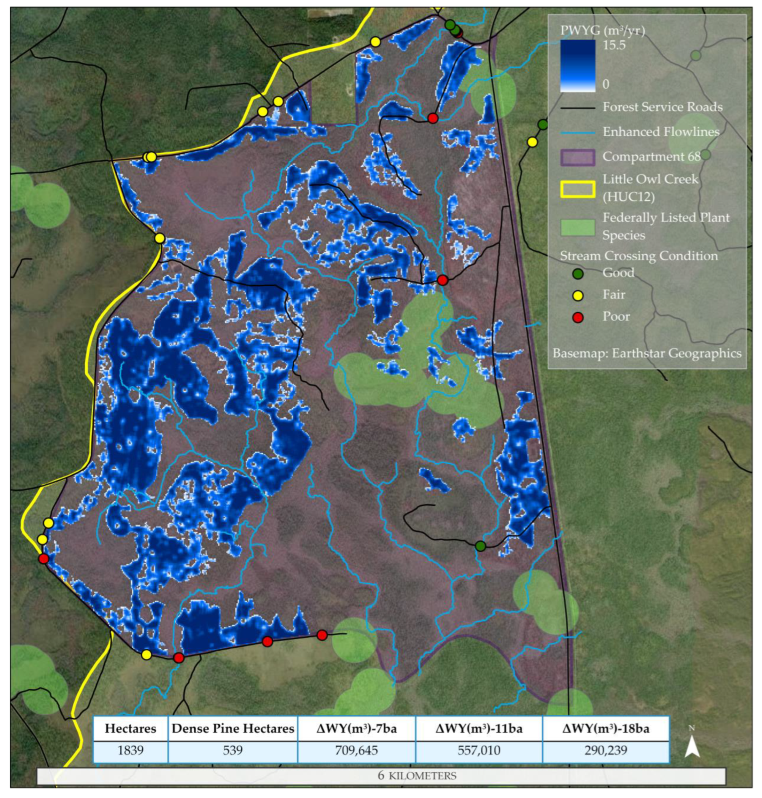
| Little Owl Creek | 12,183 | 2468 | 69.65 | 70.75 (20%) | 72.66 (45%) | 74.62 (69%) |
| ANF Compartment | ||||||
| 27 | 889 | 548 | 4.52 | 4.87 (62%) | 5.21 (85%) | 5.43 (94%) |
| 68 | 1839 | 539 | 10.20 | 10.49 (29%) | 10.88 (55%) | 11.23 (79%) |
| 73 | 1536 | 591 | 8.42 | 8.77 (39%) | 9.19 (67%) | 9.51 (78%) |
| 106 | 1083 | 466 | 6.01 | 6.24 (43%) | 6.58 (77%) | 6.84 (88%) |
| 205 | 1676 | 792 | 5.75 | 6.16 (47%) | 6.75 (89%) | 7.20 (97%) |
| 206 | 2308 | 709 | 10.08 | 10.41 (31%) | 11.06 (73%) | 11.57 (84%) |
| 217 | 1637 | 436 | 6.54 | 6.70 (27%) | 7.20 (80%) | 7.60 (93%) |
| 248 | 1307 | 416 | 4.84 | 5.03 (32%) | 5.41 (75%) | 5.71 (88%) |
| 328 | 1699 | 377 | 7.49 | 7.68 (22%) | 8.06 (63%) | 8.42 (86%) |
Disclaimer/Publisher’s Note: The statements, opinions and data contained in all publications are solely those of the individual author(s) and contributor(s) and not of MDPI and/or the editor(s). MDPI and/or the editor(s) disclaim responsibility for any injury to people or property resulting from any ideas, methods, instructions or products referred to in the content. |
© 2023 by the authors. Licensee MDPI, Basel, Switzerland. This article is an open access article distributed under the terms and conditions of the Creative Commons Attribution (CC BY) license (https://creativecommons.org/licenses/by/4.0/).
Share and Cite
Vernon, J.; St. Peter, J.; Crandall, C.; Awowale, O.E.; Medley, P.; Drake, J.; Ibeanusi, V. Spatial Application of Southern U.S. Pine Water Yield for Prioritizing Forest Management Activities. ISPRS Int. J. Geo-Inf. 2023, 12, 34. https://doi.org/10.3390/ijgi12020034
Vernon J, St. Peter J, Crandall C, Awowale OE, Medley P, Drake J, Ibeanusi V. Spatial Application of Southern U.S. Pine Water Yield for Prioritizing Forest Management Activities. ISPRS International Journal of Geo-Information. 2023; 12(2):34. https://doi.org/10.3390/ijgi12020034
Chicago/Turabian StyleVernon, Jordan, Joseph St. Peter, Christy Crandall, Olufunke E. Awowale, Paul Medley, Jason Drake, and Victor Ibeanusi. 2023. "Spatial Application of Southern U.S. Pine Water Yield for Prioritizing Forest Management Activities" ISPRS International Journal of Geo-Information 12, no. 2: 34. https://doi.org/10.3390/ijgi12020034