Article

Multi-GPU-Parallel and Tile-Based Kernel Density Estimation for Large-Scale Spatial Point Pattern Analysis

Department of Geography & the Environment, University of Denver, Denver, CO 80208, USA
*
Author to whom correspondence should be addressed.
ISPRS Int. J. Geo-Inf. 2023, 12(2), 31; https://doi.org/10.3390/ijgi12020031
Submission received: 13 November 2022 / Revised: 8 January 2023 / Accepted: 16 January 2023 / Published: 18 January 2023
(This article belongs to the Special Issue GIS Software and Engineering for Big Data)

Abstract

:
Kernel density estimation (KDE) is a commonly used method for spatial point pattern analysis, but it is computationally demanding when analyzing large datasets. GPU-based parallel computing has been adopted to address such computational challenges. The existing GPU-parallel KDE method, however, utilizes only one GPU for parallel computing. Additionally, it assumes that the input data can be held in GPU memory all at once for computation, which is unrealistic when conducting KDE analysis over large geographic areas at high resolution. This study develops a multi-GPU-parallel and tile-based KDE algorithm to overcome these limitations. It exploits multiple GPUs to speedup complex KDE computation by distributing computation across GPUs, and approaches density estimation with a tile-based strategy to bypass the memory bottleneck. Experiment results show that the parallel KDE algorithm running on multiple GPUs achieves significant speedups over running on a single GPU, and higher speedups are achieved on KDE tasks of a larger problem size. The tile-based strategy renders it feasible to estimate high-resolution density surfaces over large areas even on GPUs with only limited memory. Multi-GPU parallel computing and tile-based density estimation, while incurring very little computational overhead, effectively enable conducting KDE for large-scale spatial point pattern analysis on geospatial big data.

1. Introduction

Kernel density estimation (KDE) is a common approach to spatial point pattern analysis with applications in various fields including, but not limited to, geography, ecology, spatial epidemiology, criminology, and transportation [1,2,3,4,5]. Based on a sample set of point locations where an event of interest (e.g., crime incident) has occurred, KDE estimates event occurrence probability density at any location by averaging probability contributions from the event sample locations (Equation (1)):
f ^ ( x ) = 1 n i = 1 n 1 h i 2 K ( | x X i | h i ) e i ,
where f ^ ( x ) is the estimated probability density at foci location x, | x X i | is the Euclidean distance between x and event location Xi, and K ( · ) is a kernel function (e.g., Gaussian) with unit kernel mass (i.e., the volume under the kernel is 1.0) centered at each of the n event locations within the study area. The kernel represents a distance-decaying density contribution from an event location to the foci location (closer locations have larger contributions). hi is the bandwidth, a critical parameter that controls how quickly density decreases as distance increases. ei is the edge effect correction factor to account for the absence of event locations that are outside the study area but still contribute to probability density at the foci location. It is necessary to obtain unbiased density estimates and is calculated as the reciprocal of the kernel mass inside the study area [6]. When the study area is represented as a raster (a grid of cells), KDE can estimate event probability density cell-by-cell, which results in a density surface (raster) over the area [5]. The density raster can be readily mapped for visually inspecting the spatial pattern of the events or for quantitative analysis, for example, locating regions of unusually high and/or low occurrence density for in-depth examination [7]. Such endeavors could inform formulating hypotheses to better understand the pattern-shaping processes underlying the events. As such, KDE is a powerful tool for exploratory spatial data analysis in many application domains.
The KDE method has seen variants with new methodological developments. Unlike the above-introduced spatial KDE wherein Euclidean distance is used to measure the distance between locations and estimates densities at locations (pixels) in the planar geographic space, network KDE measures the separation between locations with network distance and estimates densities only at ‘linxels’ (line segments) in a constraining network space [2,8]. Network KDE has proven superior for analyzing point events only occurring on networks such as traffic accidents and pedestrian crashes [9,10]. Another variant is spatiotemporal KDE that considers the temporal dimension of events (e.g., timestamp) in addition to the spatial dimension (e.g., geographic coordinates). Spatiotemporal KDE estimates densities at ‘voxels’ in the space-time cube and has been used to explore the spatiotemporal patterns of a wide range of phenomena (e.g., crime and disease) [3,11,12,13].
Across all KDE methods, the choice of bandwidth is much more crucial than the choice of kernel function [14] as the bandwidth would significantly impact the smoothness of the estimated probability distribution and hence the level of generalization from the observed event sample locations to the underlying phenomenon. Generally, a larger bandwidth results in a more smoothed and generalized probability density distribution that is good for revealing the overall trends in event occurrence likelihood, whilst a smaller bandwidth leads to a distribution with more details on local variations. Moreover, bandwidth can be fixed or adaptive across event locations [5]. In contrast to fixed-bandwidth KDE wherein bandwidth stays the same at all event locations, adaptive-bandwidth KDE varies bandwidth across event locations in response to the changing local distribution pattern of event locations. For example, many human-induced point event data (e.g., alcohol store locations) tend to be much more densely distributed in populous areas than areas with sparse population. Using KDE with adaptive bandwidths that are inversely proportional to local population density produces density maps that better reflect subtle density variations in areas of dense population [15,16].
Approaches for determining KDE bandwidth, either fixed or adaptive, fall into two general categories: ‘rule-of-thumb’ heuristics and data-driven cross-validation. Following ‘rule-of-thumb’ heuristics, for instance, the fixed bandwidth for spatial KDE is calculated as a function of the standard distance of event sample locations and sample size [17], whereas adaptive bandwidths can be computed as being proportional to the k-nearest neighbor distance of each event location or similar metrics reflecting the local density of event locations [4,18,19]. Such bandwidth determination processes come with little computation overhead but still often result in oversmoothed density distribution estimations [20]. Data-driven bandwidth determination adheres to the ‘maximum likelihood principle’ and performs leave-one-out cross-validation on the event sample locations to find an optimal fixed bandwidth, or a set of optimal parameters for computing adaptive bandwidths, which maximizes the probability of observing the sample locations [5,7]. While bandwidth determined through data-driven methods usually leads to superior results, the computation processes are expensive because iterative optimizations are often involved [5,20].
Bandwidth determination is not the only step that renders KDE computationally intricate. A detailed analysis of the spatial KDE method [20] highlights other complex parts such as computing edge effect correction factors and computing probability density at large numbers of event sample locations and raster cells. The complexity of the KDE algorithm is O ( n m + n 2 ) where n is the number of event locations and m is the number of raster cells at which densities are to be estimated. As n and m increases, the run time of KDE is expected to grow quadratically to n and linearly to m. Therefore, it would be very computationally demanding to apply KDE on a large number of event locations to estimate a fine-resolution density raster over a large geographic area. In the meantime, geospatial big data are now commonplace [21], and many large-scale point datasets, such as biodiversity observations contributed by citizen science participants [22] and point-of-interest data [23], can easily exceed millions or even billions of points. Using KDE to analyze point patterns in these datasets is desirable to better understand the underlying phenomena or embedded processes [24], but such an endeavor faces immense computational challenges.
Geocomputation utilizing high-performance computing, cloud computing, advanced cyberinfrastructure, etc., has been adopted to address computational challenges facing geospatial big data analytics [25,26,27] and point pattern analysis [20,28,29]. Parallelizing spatial analysis algorithms on multi-core CPUs (central processing units) or on massive-core GPUs (graphics processing units) can significantly speed up spatial analysis tasks, although GPU-parallel computing is often much faster than CPU-based parallelization [28,29,30,31]. Specific to the spatial KDE method for point pattern analysis, the state-of-the-art GPU-parallel implementation developed by Zhang et al. [20] can complete point pattern analysis tasks tens or even hundreds of times faster than sequential computing (i.e., utilizing only a single CPU thread). It is also much faster, scalable, and flexible (for providing multiple bandwidth options) than KDE tools implemented in commonly used GIS software [24].
Nevertheless, the existing GPU-parallel KDE algorithm [20] has certain drawbacks. It supports computation with only one single GPU, whilst multiple GPUs may be available on the computing platform for further accelerating KDE computation. Moreover, it assumes that all data (points, density raster, etc.) can be held in GPU memory for computation, but in reality, geospatial big datasets could easily outsize GPU memory space. Such limitations have hindered utilizing the KDE method on point pattern analysis tasks that aim to estimate high-resolution density surfaces over large areas from massive point datasets. This study develops new extensions to improve the original GPU-parallel KDE algorithm, so it can take advantage of multiple GPUs for parallel computing and overcome the memory constraint. The new extensions are implemented in the multi-GPU-parallel and tile-based KDE, which is capable of quickly tackling ‘big’ point pattern analysis tasks. The remainder of the article is organized as follows. Section 2 provides an overview of the existing GPU-parallel KDE algorithm and identifies its drawbacks. Section 3 develops new extensions to address the drawbacks. Section 4 reports experiments for evaluating the computing performance of the multi-GPU-parallel and tile-based KDE. Section 5 and Section 6 presents the discussion and conclusion, respectively.

2. Existing GPU-Parallel KDE

2.1. Overview

KDE takes as input a set of point event locations and a raster layer depicting the extent of the study area and outputs an estimated probability density raster (Figure 1). After reading in event locations and the study area raster, fixed or adaptive bandwidths are determined at event locations. A density raster was then estimated by calculating probability density at every cell within the study area. The existing GPU-parallel KDE implementation [20] parallelizes computations involved in bandwidth determination and density raster estimation on massive GPU threads to accelerate the KDE algorithm. An overview of the existing GPU-parallel KDE algorithm is provided as follows (Figure 2), although readers interested in full details should refer to Zhang et al. [20].
The GPU-parallel KDE algorithm can run with three bandwidth options: (1) KDE with a fixed bandwidth determined using ‘rule-of-thumb’ methods, (2) KDE with a fixed bandwidth determined using cross-validation, and (3) KDE with spatially adaptive bandwidths determined using cross-validation. With the latter two bandwidth options, the algorithm first goes through a series of iterative computation steps to determine the optimal bandwidths that maximize the likelihood of observing the event locations, and finally estimates a density surface by computing densities at cells within the study area. The GPU-parallel KDE implementation adopts certain strategies to optimize the computations to effectively reduce algorithmic complexity. First, it avoids unnecessary re-computing of edge effect correction factors for points far from the study area boundary as these points should have an edge effect correction factor of 1.0, which is unlikely to change with bandwidth. Second, it uses k-dimensional tree spatial indexing to speed up distance-based queries, for example, finding points within certain search radius from a foci point. The optimizations reduce the complexity of the KDE algorithm from O ( n m + n 2 ) to O ( n m + n n ) [20].
On top of the algorithmic optimizations, calculations in each computation step are parallelized on GPU based on the CUDA (or Compute Unified Device Architecture) parallel programming library [32] to further accelerate KDE computation. For instance, computing probability density at a point is independent from computing density at another point. Thus computing densities at the points can be conducted in parallel on massive GPU threads, with each GPU thread computing density for one point. Similarly, GPU-parallel computing can also be utilized in computing density surface, where each GPU thread computes density for one cell. Computing performance of the existing GPU-parallel KDE algorithm was tested on point pattern analysis tasks involving datasets of various sizes (e.g., millions of points or raster cells), and it achieved significant speedups compared to sequential or CPU-parallel implementations (i.e., tens to hundreds of times faster) (see details in [20]).

2.2. Limitations

There are limitations to the existing GPU-parallel KDE implementation. First and foremost, it can utilize only a single GPU for parallel computing, whereas multiple GPUs may be available on the computing platform. This drawback, to certain extent, constrains the GPU-parallel KDE algorithm from being used to quickly perform point pattern analysis on large datasets. Multiple GPUs, when available, could be exploited to collaboratively parallelize computations to further speed up spatial analysis algorithms [33]. With the support of distributing computations across multiple GPUs, the KDE method would be much more capable of completing point pattern analysis tasks involving very large datasets.
Moreover, the existing GPU-parallel KDE algorithm reads into computer main memory the points and the study area raster to its full extent and transfers all the data to the memory on GPU device to perform GPU-parallel computing (e.g., computing edge effect correction factors, estimating density surface). It assumes that there is sufficiently large GPU memory space to hold all the data. While point data do not necessarily take much memory space, the size of a fine-resolution raster representing a large study area may well exceed GPU memory capacity [30,31]. For example, keeping in memory 10 million points’ geographic coordinates (e.g., x, y coordinates) needs only about 80 MB (2 coordinates per point × 4 bytes per float-number coordinate × 10 million points), but a 500-m resolution raster covering the world between latitudes 60° S and 75° N would require approximately 13.6 GB (4 bytes per float-number cell value × 80,150 columns × 42,431 rows). Many GPUs simply do not have such a large memory capacity to hold the raster. The existing GPU-parallel KDE would run out of memory and fail to estimate a high-resolution density surface over a large area. The memory constraint must be addressed so that the GPU-parallel KDE algorithm can run on GPUs with a limited amount of memory to conduct fine-resolution density estimation at large scales.

3. New Extensions to GPU-Parallel KDE

This study develops two new extensions to the existing GPU-parallel KDE algorithm, namely multi-GPU parallel computing and tile-based density estimation, to address the limitations, respectively. Multi-GPU parallel computing allows the algorithm to effectively utilize multiple GPUs to collaboratively carry out KDE computation concurrently. Tile-based density estimation enables estimating high-resolution density raster over large areas. Together, the new extensions empower the GPU-parallel KDE algorithm (source codes available at https://tinyurl.com/8jsy8ynk; accessed on 17 January 2023) for efficient large-scale spatial point pattern analysis.

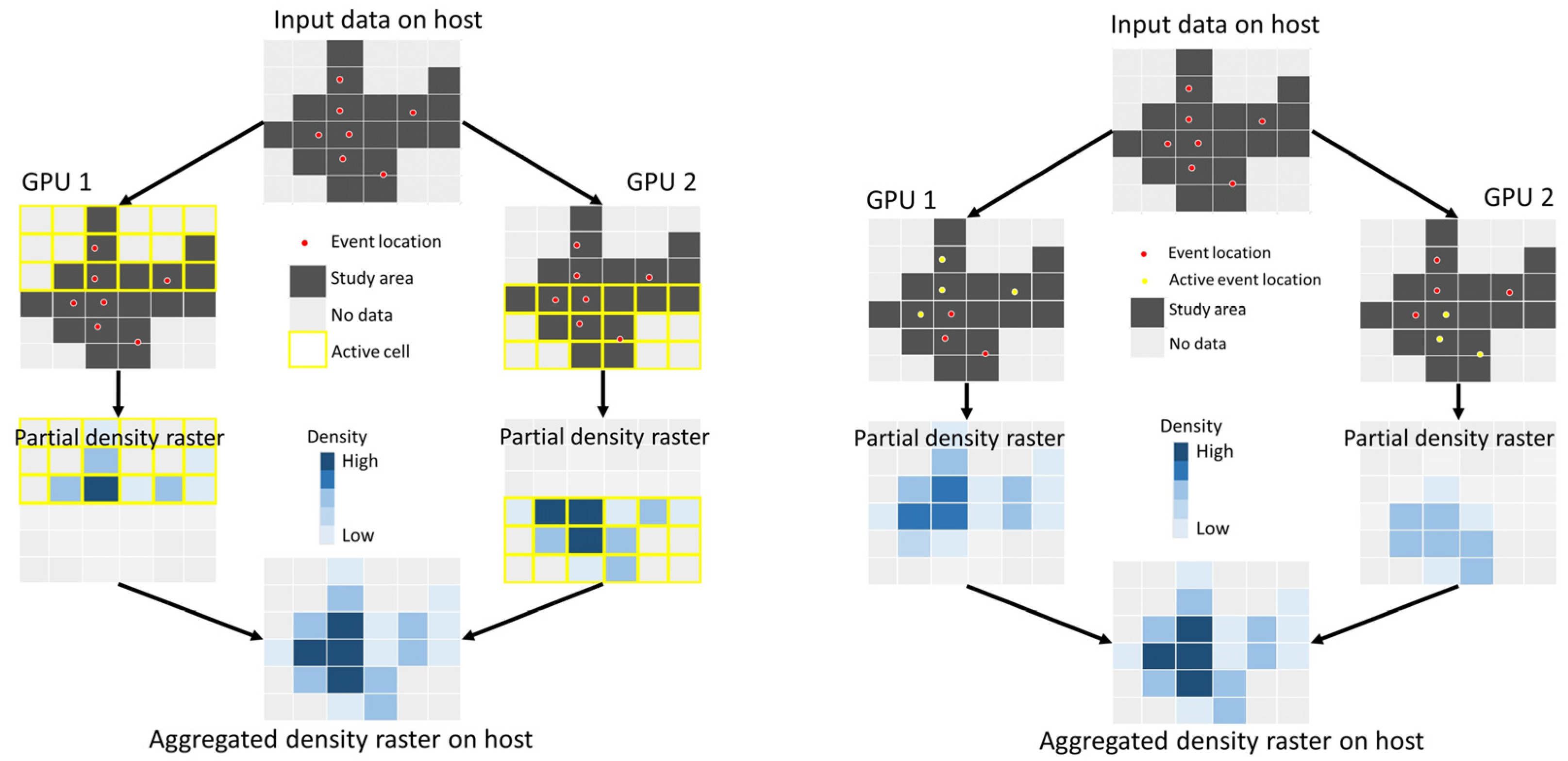
3.1. Multi-GPU Parallel Computing

Extending the existing GPU-parallel KDE algorithm to support parallel computing on multiple GPUs is a non-trivial effort. Based on the CUDA programming model [32], parallel computing threads launched on a GPU device can access only data residing in memory on that device for computation, and similarly, can write data only to its own memory. Hence, in order to utilize multiple GPUs to collaboratively complete a computation workload, the full computation workload and data needs to be partitioned into independent pieces on the host (CPU-side), which are then dispatched to multiple GPUs to be conducted concurrently. Data resulted from parallel computing on individual GPUs are then collected and transferred back to the host for further processing.
The GPU-parallel KDE exploits data parallelism for parallel computing at each computation step, meaning it maps computation on individual data items to individual GPU threads (e.g., each thread computes density at one point or at one cell) [20]. The key to multi-GPU-parallel KDE lies in properly dividing the data items (e.g., points or cells) across the GPUs, transferring the data to their respective GPU memory, launching the computing kernel on each GPU to carry out the computation on the data items that GPU is responsible for, and finally transferring results from individual GPUs back to the host where the results can be aggregated as needed.
Implementation of the multi-GPU parallel computing extension to the GPU-parallel KDE algorithm is demonstrated below through the density raster estimation step (after bandwidth determination). The input data (i.e., point locations and study area raster) are first transferred to individual GPU’s memory. Then, there are two different strategies to approach parallel density raster estimation: Cell-based parallelization or point-based parallelization (Figure 3). Taking the cell-based approach, raster cells are evenly divided (equal number of cells) across available GPUs, and each GPU’s assigned cells are marked active. A computing kernel is then launched on each GPU to estimate densities at the active cells (following Equation (1)). The kernel execution configuration on each GPU is determined based on their respective number of active cells (i.e., one GPU thread for each cell). After the kernel runs complete on all GPUs, estimated densities at their respective active cells (i.e., partial density raster) are transferred back to the host where they are spatially combined to produce a final density raster.
With point-based parallelization, points are evenly divided across available GPUs (roughly equal number of points on each GPU), and each GPU’s assigned points are marked active. A computing kernel is then launched on each GPU to compute density contributions of each point to every cells. The kernel execution configuration on each GPU is determined based on their respective number of active points (i.e., one GPU thread for each point). After kernel runs complete on all GPUs, partial density rasters are transferred back to the host where partial densities at each cell are summed up to compute a final density at that cell. Consistent with the original GPU-parallel KDE implantation [20], this parallelization strategy was adopted by default in this study, as it is computationally more efficient.
Other KDE computation steps (e.g., computing edge effect correction factors at points, computing densities at points) are similarly parallelized across multiple GPUs using the point-based approach. The Extended multi-GPU-parallel KDE automatically detects the number of GPUs available on the computing platform, divides workloads across multiple GPUs, and collects results from the GPUs for necessary aggregation. It is expected to complete KDE computation faster compared to the original single-GPU implementation, as it utilizes multiple GPUs to conduct computation concurrently.

3.2. Tile-Based Density Estimation

The study area raster is used for two purposes over the course of the KDE algorithm [20]. On the one hand, the raster depicts study area boundary, and calculating edge effect correction factors relies on it to calculate (at each event location) the kernel mass that is within the boundary. On the other hand, it serves as a geographic template of the density raster. That is, densities are estimated at every cell (except for no-data cells) in the study area raster to produce a density raster. Representing a large area at high resolution (i.e., small cell size), the study area raster may well outsize GPU memory capacity (Section 2.2). Also note that, for computing edge effect correction factors, the full extent of the raster needs to be kept in memory so the KDE algorithm can trace the entirety of the study area boundary. In contrast, estimating density raster does not require access to the full raster all at once, as density estimation at one cell is independent from that at another cell.
Accordingly, two separate user-supplied rasters can be provided as input to the KDE algorithm: one is a low-resolution raster that can easily fit into GPU memory for calculating edge effect correction factors, and the other a high-resolution raster that can be transferred to GPU memory tile-by-tile for density estimation (Figure 4). Decreasing the resolution of the study area raster for edge effect correction has negligible impact on KDE because edge effect correction factors computed based on a study area raster at a reduced resolution are not necessarily much different from those computed using a higher-resolution raster, or there is no need for edge correction if event locations outside the study area are also present [24], or users simply choose not to account for edge effect such that a (biased) density raster can be estimated much faster [20]. With the tile-based density estimation strategy, density raster over large study areas can be estimated at very high spatial resolutions, as long as the size of one raster tile fits in the GPU memory. The newly extended GPU-parallel KDE adopts GDAL (Geospatial Data Abstraction Library) to handle raster tile I/O (i.e., reading/writing tiles from/to GeoTIFF files) [34,35]. It also automatically determines the tile dimension (columns × rows) based on the amount of GPU memory available on the computing platform and the physical layout of the GeoTIFF files [30,31]. By default, a tile can use up to 20% of the memory left, and tile width and height will not exceed half of the total number of raster columns and rows, respectively, to reduce the chance of obtaining highly unbalanced tiles. Note that the computation workload of estimating densities on one raster tile is still parallelized on multiple GPUs (Section 3.1).

4. Performance Evaluation

4.1. Experiment Design

4.1.1. Overall Design and Metrics

Experiments were designed and conducted to evaluate effectiveness of the proposed extensions (i.e., multi-GPU parallel computing and tile-based density estimation) by comparing computing performance of the extended GPU-parallel KDE algorithm against the original single GPU-based implementation. The effects of the two extensions were examined through experiments (see Section 4.2 for specifics). Computing performance in this study was measured as the execution time of the algorithm to complete a given point pattern analysis task, where the total execution time is further split into I/O time (i.e., time spent on reading/writing data from/to files) and computation time (i.e., time spent on everything else, including data transfers between the host and GPUs) [20,30]. For each KDE experiment, the average execution time (i.e., total, I/O, and computation) of two repeated runs was reported.
The extended GPU-parallel KDE algorithm running parallel computing across multiple GPUs is expected to speed up KDE tasks over the original implementation that runs on only a single GPU. For a given KDE task, speedup is computed as the ratio between the computation time of the GPU-parallel KDE running a single GPU and that running on multiple GPUs (Equation (2)):
S p e e d u p = C o m p u t a t i o n _ T i m e s i n g l e _ G P U C o m p u t a t i o n _ T i m e m u l t i _ G P U
The speedup rate defined above measures how much acceleration is achieved by utilizing multiple GPUs for KDE computation compared to utilizing just a single GPU. Theoretically, the speedup should not exceed the number of GPUs in use, e.g., the maximum speedup achievable using two identical GPUs (versus using one GPU) is 2.0. One should not mistake it as the speedup achievable by GPU-based parallel KDE computation over sequential CPU-based computing, which could reach the magnitude of hundreds or even thousands. GPU over CPU speedup, however, is not the focus of this study; it has been thoroughly investigated by Zhang et al. [20].

4.1.2. Experiment Data

Synthetic datasets and real-world datasets were both used for the experiments. The extended GPU-parallel KDE algorithm can run in two different modes. In the first mode, the program uses synthetic point data and study area raster generated on-the-fly according to user specifications (Figure 5). It generates a specified number of random event locations within an artificial rectangular study area with an extent of 0–100 along the south–north direction and 0–100 along the west–east direction. The study area is discretized into a low-resolution raster for calculating edge effect correction factors and another high-resolution raster for estimating densities. The user specifies two cell sizes for the two rasters, respectively. In the second mode, data are read from user-provided data files (i.e., a CSV file containing event locations, a GeoTIFF raster file for edge effect correction, and another GeoTIFF raster for density estimation). Synthetic datasets of varying sizes (in terms of number of event locations, and number of raster cells) were used in the experiments to evaluate the effects of the two extensions on computing performance of the extended GPU-parallel KDE algorithm.
Moreover, to demonstrate the capability of the extended GPU-parallel KDE to handle authentic large-scale point pattern analysis tasks, the GPU-parallel KDE algorithm was applied to a real-world dataset containing n = 13,806,513 sampling event locations (i.e., birding sites) (Figure 6) obtained from the eBird citizen science project [36,37] for estimating 1000- or 500-m resolution probability density rasters covering the world between latitudes 60° S and 75° N.

4.1.3. Computing Platforms

Experiments were run on three computing platforms with differing computing capabilities: Dell Precision 3620 Tower, Dell Precision 5820 Tower, and Dell PowerEdge T640, hereafter referred to as the basic, intermediate, and advanced platform, respectively (Table 1). All computers run the Windows 10 operating system and have CUDA (version 11.7) and GDAL (version 3.0.0) installed and configured to run the GPU-parallel KDE algorithm. Nonetheless, they are equipped with CPUs and GPUs with different computing capabilities. The basic platform has two identical Quadro P1000 GPUs (4 GB memory each), the intermediate has two Quadro P4000 GPUs (8 GB memory each), and the advanced has one Tesla V100 GPU (32 GB memory). Due to limited resources, no computing platforms with more than two identical GPUs are available to run the experiments.

4.2. Experiments and Results

4.2.1. Effects of Multi-GPU Parallel Computing

Experiments were conducted to examine the speedup achieved by the multi-GPU version of the parallel KDE algorithm over the single-GPU version, and how various parameters of a KDE task (i.e., number of points, density raster cell size, bandwidth option, and edge effect correction) and computing platform may impact the speedup. All experiments in this section were run on the intermediate computing platform and by default without edge effect correction, unless otherwise specified. In all the experiments, the size of the study area raster did not exceed memory capacity and hence was read in all at once as a single tile for density estimation.

4.2.1.1. Impact of the Number of Points

The experiment results show computation time increases as the number of points increases, although the number of folds increased is smaller when the KDE algorithm runs on multiple GPUs compared to running on a single GPU (Table 2). For example, when the number of points increases by 10 folds from 100,000 to 1,000,000, computation time increases by 30.22 and 24.9 folds on one GPU and two GPUs, respectively. The speedup achieved on two GPUs also improves on KDE tasks involving a larger number of points. It increases from 1.58 at 100,000 points to 1.93 at 2,000,000 points, approaching the theoretical speedup of 2.0. This implies that the multi-GPU parallel computing extension effectively accelerated KDE computation and the acceleration is more significant on KDE tasks involving larger number of points.

4.2.1.2. Impact of Density Raster Cell Size

As density raster cell size decreases (i.e., number of density estimation cells increases), computation time increases. However, the number of folds increased is again smaller when the KDE algorithm runs on multiple GPUs (Table 3). As an example, when cell size is reduced from 0.5 to 0.02 and hence the number of cells increases by 625 (25 × 25) folds, computation time increases by only 20.75 and 9.4 folds on one GPU and two GPUs, respectively. The speedup achieved on two GPUs improves on KDE tasks involving more density estimation cells. It increases from 1.05 at cell size 0.2 to 1.88 at cell size 0.02, indicating that the multi-GPU extension brought more significant acceleration on KDE tasks involving larger number of density estimation cells. Noticeably, the speedup was 0.85 (below 1.0) at cell size 0.5 (i.e., computation was slower on two GPUs), which may suggest that the benefits of multi-GPU computation outweigh its associated costs on KDE tasks only beyond certain problem size (more in Section 5.1).

4.2.1.3. Impact of Bandwidth Option

Density rasters estimated with fixed or adaptive bandwidths determined based on cross-validation are more capable of revealing fine-scale density variabilities (Figure 7). Nonetheless, determining bandwidth through cross-validation is much more computationally expensive than using the simple ‘rule-of-thumb’ method (Table 4). Utilizing one GPU, the computing time of KDE with cross-validated fixed bandwidth and with adaptive bandwidths increases by 3.28 and 20.3 folds compared to KDE with ‘rule-of-thumb’ bandwidth, respectively, whilst utilizing two GPUs, the number of folds increased in computation time is 2.74 and 15.87, respectively. The speedup achieved on two GPUs improves from 1.52 on KDE with ‘rule-of-thumb’ bandwidth to 1.92 with adaptive bandwidths, suggesting the multi-GPU extension achieved more significant acceleration on KDE tasks involving more complex bandwidth determination methods.

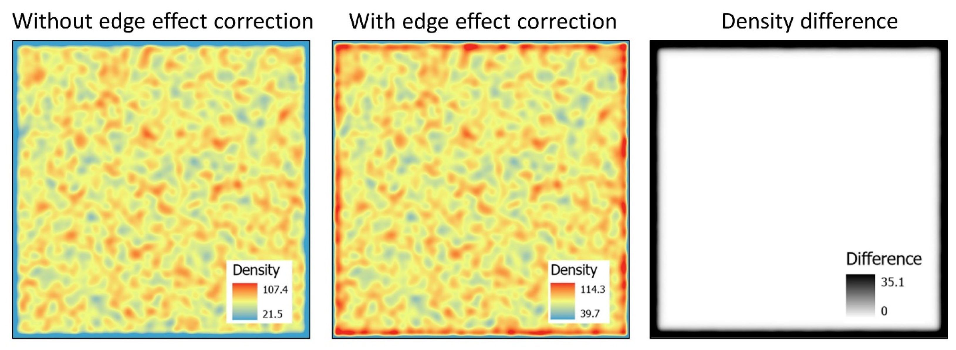
4.2.1.4. Impact of Edge Effect Correction

Edge effect correction may be necessary to obtain unbiased density estimates, especially at estimation locations close the boundary of the study area, when event locations outside the study area are not present (Figure 8). However, it incurs significant extra computational workload. With edge effect correction, the computation time of KDE with cross-validated fixed bandwidth and with adaptive bandwidths (Table 5) increases by roughly 3 and 18 folds compared to their KDE counterparts without edge correction (Table 4). Utilizing one GPU, the computing time of KDE with cross-validated fixed bandwidth and with adaptive bandwidths increases by 9.21 and 344.7 folds, respectively, compared to KDE with ‘rule-of-thumb’ bandwidth. Utilizing two GPUs, the number of folds increased in computation time is 7.83 and 288.39, respectively. Nevertheless, the speedup achieved on two GPUs improves from 1.61 on KDE with ‘rule-of-thumb’ bandwidth to 1.92 with adaptive bandwidths, implying that the multi-GPU extension still brings more significant acceleration on KDE tasks with complex bandwidth determination methods even when computationally expensive edge effect correction is carried out.

4.2.1.5. Impact of Computing Platforms

Completing the same KDE task on a synthetic dataset, the computation time on the intermediate and advanced platforms decreases by 2.97 and 12.57 folds, respectively, compared to that on the basic platform (Table 6). This is expected as the three platforms, from basic to advanced, are equipped with increasingly capable GPUs. Nonetheless, utilizing two GPUs on the basic and intermediate platforms both achieved a speedup of 1.92 (the maximum theoretical speedup is 2.0), suggesting compatibility and good performance of the multi-GPU-parallel KDE algorithm across platforms of varying computing capability.

4.2.2. Effects of Tile-Based Density Estimation

A synthetic dataset with 1,000,000 points in the artificial study area (represented as a raster at 0.005 cell size) was used to test the effectiveness of the tile-based density estimation strategy (Table 7). The study area raster for density estimation has 400 million cells (20,000 × 20,000), which requires about 1.5 GB GPU memory space (4 bytes per float-number cell value × 400 million cells). Whilst the Tesla GPU with 32 GB memory on the advanced computing platform could easily hold the whole raster in its memory as a single tile, the basic platform can only process the raster tile-by-tile, because the Quadro P1000 GPU therein has only 4 GB of memory, which also holds other data such as points, and by default only 20% of the memory left can be used for the raster tile. While the execution time was longer on the basic platform than on the advanced platform (I/O and computation time was 2.6 and 9.8 times as long, respectively), the GPU-parallel KDE algorithm was able to estimate the density rater in nine tiles on the basic platform. Enabled by the tile-based density estimation extension, the GPU-parallel KDE algorithm can now complete KDE tasks that involve density rasters larger than the GPU memory.

4.2.3. Point Pattern Analysis on the eBird Dataset

The multi-GPU-parallel and tile-based KDE algorithm was applied to the eBird dataset for density estimation with different bandwidth options and on different computing platforms to evaluate its usability on authentic large-scale point pattern analysis tasks. Density raster maps covering the world land areas between latitudes 60° S and 75° N were estimated with fixed bandwidth using all n = 13,806,513 eBird sampling locations at 1 km or 500 m spatial resolution. The space needed to store the full raster size in memory is approximately 3.4 GB at 1 km resolution (4 bytes per float-number cell value × 40,075 columns × 21,215 rows) and 13.6 GB at 500 m resolution (4 bytes per float-number cell value × 80,150 columns × 42,431 rows). A density raster map was estimated with adaptive bandwidths at 30 m resolution in a focus area (Colorado, United States) based on extracted eBird sampling locations within and around the study area (n = 324,983 points). For the focus area, the full raster size in memory is approximately 2.1 GB (4 bytes per float-number cell value × 27,090 columns × 19,760 rows). Edge effect correction is not necessary in these KDE cases because sampling locations beyond the study area boundaries are present in the dataset.

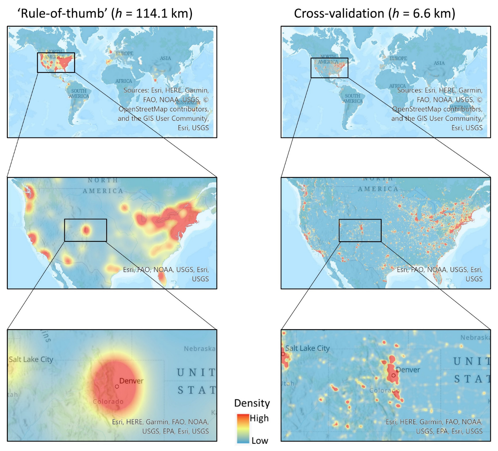
4.2.3.1. KDE with Fixed Bandwidth

As expected, the ‘rule-of-thumb’ bandwidth leads to over-smoothed density estimates that are good for revealing eBird sampling density trends at larger spatial scales (e.g., global, continental), whilst the cross-validated fixed bandwidth better captures sampling density variations at smaller scales (e.g., regional, metropolitan) (Figure 9) [24]. Regarding execution time for estimation at 1 km resolution (Table 8), consistent with the results from experiments using synthetic datasets, determining bandwidths through cross-validation incurs much more computation workload compared to using the simple ‘rule-of-thumb’ method. The computation time increases by about 12 and 19 folds on the intermediate and advanced platforms, respectively. However, the speedup achieved by utilizing two GPUs improves from 1.95 to 1.99, closely approaching the theoretical maximum of 2.0. Estimating density at 500 m resolution (Table 9), it took about 8 h (in 32 tiles) on the basic platform using two GPUs and 2 h (in 8 tiles) on the advanced platform, roughly a 4 folds increase from density estimation at 1 km resolution. The results indicate that the extended GPU-parallel KDE algorithm can effectively handle large-scale point pattern analysis tasks by dividing-and-conquering the problem using the tile-based density estimation strategy and by exploiting parallel computing power on multiple GPUs.

4.2.3.2. KDE with Adaptive Bandwidths

Compared to the 1-km resolution density map estimated with cross-validated fixed bandwidth, the 30-m resolution density map estimated with adaptive bandwidths can reveal density variations at even finer spatial scales (e.g., neighborhood) (Figure 10) [24]. As for execution time (Table 10), estimating the 30-m density map (in 9 tiles) with adaptive bandwidths can be completed in about 79 and 29 min on the basic and intermediate platforms (using two GPUs), respectively, and in 11 min on the advanced platform. The speedup achieved by utilizing two GPUs was 1.86 and 1.9 on the basic and intermediate platforms, respectively. Further, it shows that the tile-based density estimation and multi-GPU parallel computing extensions can enable fine-resolution density estimation with the computationally intricate adaptive bandwidth determination method.

5. Discussion

5.1. Cost-Benefit Analysis of the New Extensions

The multi-GPU parallel computing and the tile-based density estimation extensions, on the one hand, come with some overhead. First, multi-GPU parallel computing incurs extra cost on frequently transferring data between the host and multiple GPUs. For example, when iteratively determining the optimal adaptive bandwidths [20], at each iteration, densities at sample locations are estimated on multiple GPUs (e.g., utilizing two GPUs, each GPU is responsible for computing densities at half of the locations). The partial density arrays on each GPU are then copied to the host to form a complete density array, which is then copied back to the GPUs for computing updated bandwidths to compute density estimates at the next iteration. To assess such a data transfer cost, the time spent on every data transfer between the host and GPUs were recorded for the experiment of estimating 30-m resolution density raster on the basic computing platform with adaptive bandwidths in Colorado using eBird data. Results show moving data back-and-forth between the host and GPUs are very fast given the high peak memory bandwidth on modern GPUs (e.g., Table 1). It took only 2.22 and 6.52 s to transfer data between the host and one GPU and between the host and two GPUs, respectively. Data transfer cost increases when more GPUs are involved, but it remains negligible compared to the total execution time (147.96 and 78.79 min, respectively; Table 10). Even with a larger number of GPUs (e.g., more than two), data transfer cost is not expected to increase the execution time in any significant way.
Second, tile-based density estimation also incurs extra cost on reading/writing data multiple times from/to the raster file. Nonetheless, across all experiments in this study, I/O time is much less than computation time, seldomly exceeding 5% of the total execution time. In addition, I/O cost is determined by host characteristics (e.g., disk I/O speed). It does not correlate with the cost of data transfer among GPUs (i.e., utilizing a larger number of GPUs does not increase I/O cost).
However, the benefits of the two extensions are apparent. Multi-GPU parallel computing effectively exploits computing resources on multiple GPUs, with the speedup rate approaching the theoretical maximum, to speed up complex KDE computation involving very large numbers of points and density estimation cells. Tile-based density estimation overcomes memory constraint and makes it feasible to estimate densities at high spatial resolutions over large areas. The extensions should scale well to a larger number of GPUs, as analyzed above. Overall, the two extensions are highly cost-effective and scalable to handle large-scale point pattern analysis on massive datasets.

5.2. Recommendations on Using GPU-Parallel KDE

Experiment results have demonstrated that the multi-GPU-parallel and tile-based KDE algorithm is capable of handling very large-scale point pattern analysis tasks. It could be a useful tool for discovering patterns embedded in massive geographic point datasets to shed light on the underlying spatial processes [24,38]. Here are a few recommendations for users to effectively adopt this computational tool for their own application scenarios.
First and foremost, decide on an appropriate bandwidth option. Making such a decision requires careful consideration of the methodological and computational implications. Fixed bandwidth determined based on simple ‘rule-of-thumb’ methods, although it almost always leads to over-smoothed density estimates informative of patterns at coarse spatial granularity, is most convenient computationally. In contrast, fixed bandwidth determined through data-driven methods (e.g., cross-validation) often is able to capture density variations at finer spatial scales, but the computational processes are more involved. Determining adaptive bandwidths through data-driven methods, however, is computationally the most complicated but it results in density surfaces that can reveal patterns at the finest spatial granularity among the three bandwidth options. When the number of event locations is relatively small (e.g., a couple million points), any bandwidth option is feasible as KDE computation can be completed fairly quickly. For a large-scale point pattern analysis task (e.g., tens of millions of points), however, bandwidth (fixed or adaptive) determination through cross-validation on the full dataset may become burdensome due to the elongated execution time.
In such cases, users are advised to approach the KDE task at hand in one of the two following ways. (1) The GPU-parallel KDE offers an option to directly read bandwidths from the point data file. The user can thus run KDE with a progression of fixed bandwidths on the full dataset to identify an appropriate bandwidth that produces a satisfactory density surface. As an example, Zhang [24] utilized KDE with a series of bandwidths (e.g., 1/2, 1/4, 1/8, …, 1/128 of the ‘rule-of-thumb’ bandwidth) to generate density surfaces with varying levels of detail for detecting and visualizing hot-spots in massive point data across spatial scales. (2) Zoom in to a focus study area and run KDE with fixed or adaptive bandwidths determined through cross-validation on only data points within and around the focus area. This proves to be a reasonable compromise between the methodological and computational implications, as the advantage of cross-validated bandwidths happens to lie in revealing fine-scale density variations in local areas (Section 4.2.3.2; [24]).
The second is regarding whether to run KDE with edge effect correction [6]. Edge effect correction, even with a low-resolution study area boundary raster, incurs significant computational overhead (Section 4.2.1.4; [20]). Hence, wherever possible, it should be avoided, or its cost be reduced as much as possible. To re-iterate, edge effect correction can be omitted, for example, in the following situations. (1) Event locations (points) outside the density raster boundary are also present in the dataset, so there is no need for edge effect correction (e.g., experiments in Section 4.2.3). (2) Users deem a density surface with slight density estimation biases near the boundary still suits the application purpose and thus prefer shorter execution time over accurate density estimation. In cases where edge correction is absolutely necessary, users can still reduce its associated computational cost by using a low-resolution raster to represent the study area boundary to more quickly compute the approximate edge correction factors [28].

5.3. Point Pattern Analysis versus Heat Map Visualization

The KDE algorithm in this study was adopted to estimate a density raster covering a geographic study area at a certain spatial resolution (i.e., a grid of cells, each with an estimated probability density value indicating the likelihood of the event occurring at the cell location) based on a set of point event locations, with properly determined bandwidths, and with edge effect accounted for where necessary (Equation (1)). The output density raster is specifically intended to aid spatial point pattern analysis, which can be carried out in a variety of ways. Event hotspots can be extracted from the density raster using quantitative methods, for example, by simply applying a density threshold (i.e., cells with density above the threshold are regarded as hotspot areas). Alternatively, the estimated density raster can be visualized as a density map (i.e., “heat” map) for visually (thus qualitatively) locating hotspots, which can be performed in regular GIS software and in an interactive manner (e.g., zoom in, zoom out, and pan).
Rendering heat maps is never the ultimate goal, but rather a byproduct of KDE in the context of geographic point pattern analysis [5], although KDE has been used extensively for heat map visualization as a general way of summarizing a large amount of point data. Strategies have been developed to address the computation challenges associated with KDE-based heat map generation from big point data, for example, by utilizing big data infrastructure [39] and streaming computing [40], and by computing approximate, instead of exact, densities to reduce computing complexity [41]. These strategies could potentially accelerate KDE for point pattern analysis as well. However, several differences between the two KDE application scenarios may render the strategies not readily transferrable to point pattern analysis. First, density estimation in heat map visualization usually does not involve edge effect correction as it is not constrained by a geographic study area. Second, heat map visualization generally do not offer flexible bandwidth options (e.g., adaptive bandwidths). Third, heat map visualization often generates maps only for display (e.g., on computer screens) and densities are computed on-the-fly only at a small number of display pixels (e.g., 1280 × 960 pixels) at the current zoom level [42]. In contrast, density estimation for point pattern analysis could be at high-resolution over a large area (e.g., 80,150 × 42,431 cells at 500 m resolution covering the world between latitudes 60° S and 75° N; Section 4.2.3). Moreover, for heat map visualization, there may be no need to save densities at locations beyond the pixels within the current display extent, which greatly reduces memory demand, but for point pattern analysis the full extent density raster needs to be tracked.

6. Conclusions

This study develops a new GPU-parallel KDE algorithm that supports multi-GPU parallel computing and tile-based density estimation for large-scale point pattern analysis (e.g., massive points, large area, and high resolution). By dividing computation workload across GPUs, it can exploit computing resources on multiple GPUs to speedup complex KDE computation. The tile-based processing strategy addresses the memory bottleneck facing KDE over large areas at high spatial resolution. The results of the experiments conducted on platforms with differing computing capability confirm that the multi-GPU parallel KDE algorithm achieves significant speedup over the single GPU version. It achieves higher speedups, approaching the maximum theoretical speedup, on KDE tasks of a larger problem size (e.g., KDE tasks involving a larger number of points and/or density estimation cells, more complicated bandwidth determination mechanisms, and expensive edge effect correction). Moreover, the tile-based strategy towards density estimation renders it feasible to run the parallel KDE algorithm on computers with only limited GPU memory to complete ‘big’ KDE tasks (e.g., estimating a global 500-m resolution density raster based on tens of millions of eBird sampling locations). The scalable multi-GPU parallel computing and tile-based density estimation features, while incurring very little computational overhead, effectively enable the GPU-parallel KDE algorithm for large-scale spatial point pattern analysis on geospatial big data with the KDE method.
Due to limited resources, this study did not test the performance of the multi-GPU parallel KDE algorithms on more than two identical GPUs, although analyses suggest that it should scale well to a larger number of GPUs (Section 5.1). Another potential improvement on the current multi-GPU parallel KDE algorithms is to further extend it to support utilizing GPUs available on a network of compute nodes so it is even more capable of handling massive KDE tasks. The algorithm now only uses GPUs on the same computer for parallel computing, which was implemented based on the CUDA programming library. If it were to access GPUs on more than one compute nodes, more complex cross-computer programming libraries such as CUDA-aware MPI (message passing interface) (https://developer.nvidia.com/blog/introduction-cuda-aware-mpi/; accessed on 17 January 2023) would be needed for implementation, and additional cost of transferring data across nodes (for both GPU computation and I/O) is expected to be incurred.

Author Contributions

Conceptualization, methodology, data curation, analysis, writing—original draft preparation, and revision, Guiming Zhang; methodology, data analysis, writing—review and editing, Jin Xu. All authors have read and agreed to the published version of the manuscript.

Funding

This research was supported by the Faculty Research Fund (FRF) grant and the Professional Research Opportunities for Faculty (PROF) grant at the University of Denver.

Data Availability Statement

eBird observations were downloaded from the eBird website at https://ebird.org/data/download (accessed on 30 August 2022). Source codes of the multi-GPU-parallel and tiled KDE algorithm are available on GitHub at https://tinyurl.com/8jsy8ynk (accessed on 17 January 2023).

Acknowledgments

The author thanks the eBird project for making its data freely available and the many eBirders for contributing birding records.

Conflicts of Interest

The authors declare no conflict of interest.

References

  1. Shi, X.; Li, M.; Hunter, O.; Guetti, B.; Andrew, A.; Stommel, E.; Bradley, W.; Karagas, M. Estimation of environmental exposure: Interpolation, kernel density estimation or snapshotting. Ann. GIS 2019, 25, 1–8. [Google Scholar] [CrossRef] [PubMed] [Green Version]
  2. Xie, Z.; Yan, J. Kernel Density Estimation of traffic accidents in a network space. Comput. Environ. Urban Syst. 2008, 32, 396–406. [Google Scholar] [CrossRef] [Green Version]
  3. Nakaya, T.; Yano, K. Visualising crime clusters in a space-time cube: An exploratory data-analysis approach using space-time kernel density estimation and scan statistics. Trans. GIS 2010, 14, 223–239. [Google Scholar] [CrossRef]
  4. Yuan, K.; Chen, X.; Gui, Z.; Li, F.; Wu, H. A quad-tree-based fast and adaptive Kernel Density Estimation algorithm for heat-map generation. Int. J. Geogr. Inf. Sci. 2019, 33, 2455–2476. [Google Scholar] [CrossRef]
  5. Brunsdon, C. Estimating probability surfaces for geographical point data: An adaptive kernel algorithm. Comput. Geosci. 1995, 21, 877–894. [Google Scholar] [CrossRef]
  6. Diggle, P. A Kernel Method for Smoothing Point Process Data. J. R. Stat. Soc. Ser. C (Appl. Stat.) 1985, 34, 138–147. [Google Scholar] [CrossRef]
  7. van Dijk, J.; Longley, P.A. Interactive display of surnames distributions in historic and contemporary Great Britain. J. Maps 2020, 16, 68–76. [Google Scholar] [CrossRef] [Green Version]
  8. Okabe, A.; Satoh, T.; Sugihara, K. A kernel density estimation method for networks, its computational method and a GIS-based tool. Int. J. Geogr. Inf. Sci. 2009, 23, 7–32. [Google Scholar] [CrossRef]
  9. Xie, Z.; Yan, J. Detecting traffic accident clusters with network kernel density estimation and local spatial statistics: An integrated approach. J. Transp. Geogr. 2013, 31, 64–71. [Google Scholar] [CrossRef]
  10. Dai, D.; Taquechel, E.; Steward, J.; Strasser, S. The impact of built environment on pedestrian crashes and the identification of crash clusters on an urban university campus. West. J. Emerg. Med. 2010, 11, 294. [Google Scholar]
  11. Hohl, A.; Tang, W.; Casas, I.; Shi, X.; Delmelle, E. Detecting space–time patterns of disease risk under dynamic background population. J. Geogr. Syst. 2022, 24, 389–417. [Google Scholar] [CrossRef] [PubMed]
  12. Lee, J.; Gong, J.; Li, S. Exploring spatiotemporal clusters based on extended kernel estimation methods. Int. J. Geogr. Inf. Sci. 2017, 31, 1154–1177. [Google Scholar]
  13. Delmelle, E.; Dony, C.; Casas, I.; Jia, M.; Tang, W. Visualizing the impact of space-time uncertainties on dengue fever patterns. Int. J. Geogr. Inf. Sci. 2014, 28, 1107–1127. [Google Scholar] [CrossRef]
  14. Silverman, B.W. Density Estimation for Statistics and Data Analysis; Chapman and Hall: London, UK, 1986. [Google Scholar]
  15. Carlos, H.A.; Shi, X.; Sargent, J.; Tanski, S.; Berke, E.M. Density estimation and adaptive bandwidths: A primer for public health practitioners. Int. J. Health Geogr. 2010, 9, 39. [Google Scholar] [CrossRef] [PubMed] [Green Version]
  16. Shi, X. Selection of bandwidth type and adjustment side in kernel density estimation over inhomogeneous backgrounds. Int. J. Geogr. Inf. Sci. 2010, 24, 643–660. [Google Scholar] [CrossRef]
  17. Fotheringham, A.S.; Brunsdon, C.; Charlton, M. Quantitative Geogr. Perspectives on Spatial Data Analysis; Sage: Thousand Oaks, CA, USA, 2000; ISBN 1847876412. [Google Scholar]
  18. Breiman, L.; Meisel, W.; Purcell, E. Variable kernel estimates of multivariate densities. Technometrics 1977, 19, 135–144. [Google Scholar] [CrossRef]
  19. Abramson, I.S. On bandwidth variation in kernel estimates-A square root law. Ann. Stat. 1982, 10, 1217–1223. [Google Scholar] [CrossRef]
  20. Zhang, G.; Zhu, A.-X.; Huang, Q. A GPU-accelerated adaptive kernel density estimation approach for efficient point pattern analysis on spatial big data. Int. J. Geogr. Inf. Sci. 2017, 31, 2068–2097. [Google Scholar] [CrossRef]
  21. Lee, J.-G.; Kang, M. Geospatial Big Data: Challenges and Opportunities. Big Data Res. 2015, 2, 74–81. [Google Scholar] [CrossRef]
  22. Zhang, G. Spatial and Temporal Patterns in Volunteer Data Contribution Activities: A Case Study of eBird. ISPRS Int. J. Geo-Inf. 2020, 9, 597. [Google Scholar] [CrossRef]
  23. Psyllidis, A.; Gao, S.; Hu, Y.; Kim, E.-K.; McKenzie, G.; Purves, R.; Yuan, M.; Andris, C. Points of Interest (POI): A commentary on the state of the art, challenges, and prospects for the future. Comput. Urban Sci. 2022, 2, 20. [Google Scholar] [CrossRef] [PubMed]
  24. Zhang, G. Detecting and visualizing observation hot-spots in massive volunteer-contributed geographic data across spatial scales using GPU-accelerated kernel density estimation. ISPRS Int. J. Geo-Inf. 2022, 11, 55. [Google Scholar] [CrossRef]
  25. Wu, H.; Zhang, T.; Gong, J. GeoComputation for Geospatial Big Data. Trans. GIS 2014, 18, 1–2. [Google Scholar] [CrossRef]
  26. Yang, C. Utilizing Cloud Computing to Address Big Geospatial Data Challenges. Comput. Environ. Urban Syst. 2017, 61, 120–128. [Google Scholar] [CrossRef] [Green Version]
  27. Wang, S. A CyberGIS framework for the synthesis of Cyberinfrastructure, GIS, and spatial analysis. Ann. Assoc. Am. Geogr. 2010, 100, 535–557. [Google Scholar] [CrossRef]
  28. Zhang, G.; Huang, Q.; Zhu, A.-X.; Keel, J. Enabling point pattern analysis on spatial big data using cloud computing: Optimizing and accelerating Ripley’s K function. Int. J. Geogr. Inf. Sci. 2016, 30, 2230–2252. [Google Scholar] [CrossRef]
  29. Tang, W.; Feng, W.; Jia, M. Massively parallel spatial point pattern analysis: Ripley’s K function accelerated using graphics processing units. Int. J. Geogr. Inf. Sci. 2015, 29, 412–439. [Google Scholar] [CrossRef]
  30. Zhang, G. PyCLKDE: A big data-enabled high-performance computational framework for species habitat suitability modeling and mapping. Trans. GIS 2022, 26, 1754–1774. [Google Scholar] [CrossRef]
  31. Zhang, G.; Zhu, A.-X.; Liu, J.; Guo, S.; Zhu, Y. PyCLiPSM: Harnessing heterogeneous computing resources on CPUs and GPUs for accelerated digital soil mapping. Trans. GIS 2021, 25, 1396–1418. [Google Scholar] [CrossRef]
  32. Luebke, D. CUDA: Scalable parallel programming for high-performance scientific computing. In Proceedings of the 2008 5th IEEE International Symposium on Biomedical Imaging: From Nano to Macro, Paris, France, 14–17 May 2008; pp. 836–838. [Google Scholar]
  33. Shi, X.; Ye, F. Kriging interpolation over heterogeneous computer architectures and systems. GIScience Remote Sens. 2013, 50, 196–211. [Google Scholar] [CrossRef]
  34. Warmerdam, F. The Geospatial Data Abstraction Library. In Open Source Approaches in Spatial Data Handling; Hall, G.B., Leahy, M.G., Eds.; Springer: Berlin/Heidelberg, Germany, 2008; pp. 87–104. ISBN 978-3-540-74831-1. [Google Scholar]
  35. Qin, C.-Z.; Zhu, L.-J. GDAL/OGR and Geospatial Data IO Libraries. In The Geographic Information Science & Technology Body of Knowledge. 2020. Available online: https://gistbok.ucgis.org/bok-topics/gdalogr-and-geospatial-data-io-libraries (accessed on 30 August 2022).
  36. eBird. eBird Basic Dataset Metadata (v1.13). 2021. Available online: https://ebird.org/data/download/ebd (accessed on 30 August 2022).
  37. Sullivan, B.L.; Aycrigg, J.L.; Barry, J.H.; Bonney, R.E.; Bruns, N.; Cooper, C.B.; Damoulas, T.; Dhondt, A.A.; Dietterich, T.; Farnsworth, A.; et al. The eBird enterprise: An integrated approach to development and application of citizen science. Biol. Conserv. 2014, 169, 31–40. [Google Scholar] [CrossRef]
  38. Stein, A.; Detotto, C.; Belgiu, M. A spatial statistical study of the distribution of Sardinian nuraghes. Ann. GIS 2022, 28, 245–262. [Google Scholar] [CrossRef]
  39. Perrot, A.; Bourqui, R.; Hanusse, N.; Lalanne, F.; Auber, D. Large interactive visualization of density functions on big data infrastructure. In Proceedings of the 2015 IEEE 5th Symposium on Large Data Analysis and Visualization (lDAV), Chicago, IL, USA, 25–26 October 2015; pp. 99–106. [Google Scholar]
  40. Perrot, A.; Bourqui, R.; Hanusse, N.; Auber, D. HeatPipe: High throughput, low latency big data heatmap with spark streaming. In Proceedings of the 2017 21st International Conference Information Visualisation (IV), London, UK, 11–14 July 2017; pp. 66–71. [Google Scholar]
  41. Chan, T.N.; Cheng, R.; Yiu, M.L. QUAD: Quadratic-Bound-based Kernel Density Visualization. In Proceedings of the 2020 ACM SIGMOD International Conference on Management of Data, Portland, OR, USA, 14–19 June 2020; pp. 35–50. [Google Scholar]
  42. Chan, T.N.; Ip, P.L.; U, L.H.; Tong, W.H.; Mittal, S.; Li, Y.; Cheng, R. KDV-Explorer: A near real-time kernel density visualization system for spatial analysis. Proc. VLDB Endow. 2021, 14, 2655–2658. [Google Scholar] [CrossRef]
Figure 1. An illustration of KDE input (left) and output (right). Probability densities are estimated at raster cells that are within the study area, except for no-data cells.
Ijgi 12 00031 g001
Figure 2. Computation steps in the existing GPU-parallel KDE algorithm.
Ijgi 12 00031 g002
Figure 3. Cell-based parallelization (left) and point-based parallelization (right) of density raster estimation using multiple GPUs. Here, as an example, only two GPUs are used in the figure while the strategies apply to any number of GPUs.
Ijgi 12 00031 g003
Figure 4. The extended GPU-parallel KDE algorithm estimates density raster one tile at a time.
Ijgi 12 00031 g004
Figure 5. An example synthetic dataset (left) containing n = 500 random event locations in the rectangular study area discretized into a 10,000 rows × 10,000 columns raster (cell size 0.1) for density estimation, and the density raster (right) estimated with fixed bandwidths h = 7.668 determined using the ‘rule-of-thumb’ method.
Ijgi 12 00031 g005
Figure 6. eBird sampling event locations in 2021 (n = 13,806,513).
Ijgi 12 00031 g006
Figure 7. Density rasters estimated with different bandwidth options on a synthetic dataset (n = 1,000,000 points; density raster cell size = 0.05).
Ijgi 12 00031 g007
Figure 8. Density rasters estimated using ‘rule-of-thumb’ fixed bandwidth with or without edge effect correction, and their differences on a synthetic dataset (n = 1,000,000 points; density raster cell size = 0.05).
Ijgi 12 00031 g008
Figure 9. Density maps estimated with fixed bandwidth determined through the ‘rule-of-thumb’ method and through cross-validation on the eBird dataset between (n = 13,806,513 points; density raster cell size = 1 km).
Ijgi 12 00031 g009
Figure 10. Comparison of the density map estimated with fixed bandwidth (cross-validation) and adaptive bandwidths in Colorado and a zoom-in area in the Denver metropolitan area.
Ijgi 12 00031 g010
Table 1. Specifications of the three computing platforms.
PlatformCPUGPU
Precision 3620
(Basic)
Intel Core i7 CPUNVIDIA Quadro P1000 × 2
3.6 GHz max clock speed1.48 GHz max clock speed
4 cores (8 logical processors)4 GB memory
16 GB memory80 GB/s peak memory bandwidth
Precision 5820
(Intermediate)
Intel Xeon CPUNVIDIA Quadro P4000 × 2
3.7 GHz max clock speed1.48 GHz max clock speed
8 cores (16 logical processors)8 GB memory
64 GB memory243 GB/s peak memory bandwidth
PowerEdge T640
(Advanced)
Intel Xeon CPUNVIDIA Tesla V100 × 1
2.7 GHz max clock speed1.38 GHz max clock speed
24 cores (48 logical processors)32 GB memory
192 GB memory898 GB/s peak memory bandwidth
Table 2. Execution time (in seconds) for density estimation with adaptive bandwidths on synthetic datasets (varied number of points; density raster cell size = 0.05).
# Points# GPUsTotalI/OComputation# Folds Increased Speedup
100,000131.670.1731.501.00
220.100.1719.921.001.58
200,000185.450.1685.292.71
245.890.1745.722.291.87
500,0001281.410.19281.228.93
2152.290.20152.097.631.85
1,000,0001952.000.17951.8330.22
2496.350.18496.1624.901.92
2,000,00012237.940.152237.7971.04
21159.770.171159.6058.201.93
Table 3. Execution time (in seconds) for density estimation with ‘rule-of-thumb’ fixed bandwidth on synthetic datasets (n = 1,000,000 points; varied density raster cell size).
Cell Size# GPUsTotalI/OComputation# Folds Increased Speedup
0.5111.300.0011.291.00
213.240.0013.231.000.85
0.2113.240.0113.231.17
212.670.0212.650.961.05
0.1120.690.0820.621.83
217.870.0617.811.351.16
0.05147.670.1547.514.21
231.470.2131.262.361.52
0.021235.491.09234.4120.75
2125.651.27124.389.401.88
Table 4. Execution time (in seconds) for density estimation with three bandwidth options on a synthetic dataset (n = 1,000,000 points; density raster cell size = 0.05).
Bandwidth Option# GPUsTotalI/OComputation# Folds IncreasedSpeedup
Fixed bandwidth
(‘rule-of-thumb’)
147.670.1547.511.00
231.470.2131.261.001.52
Fixed bandwidth
(cross-validation)
1155.790.16155.633.28
285.720.1785.552.741.82
Adaptive bandwidths
(cross-validation)
1952.000.17951.8320.03
2496.350.18496.1615.871.92
Table 5. Execution time (in seconds) for density estimation with edge effect correction on a synthetic dataset (n = 1,000,000 points; density raster cell size = 0.05).
Bandwidth Option# GPUsTotalI/OComputation# Folds IncreasedSpeedup
Fixed bandwidth
(‘rule-of-thumb’)
150.070.1649.911.00
231.160.1531.011.001.61
Fixed bandwidth
(cross-validation)
1459.670.16459.519.21
2242.920.17242.757.831.89
Adaptive bandwidths
(cross-validation)
117,203.410.1817,203.23344.70
28941.880.198941.69288.391.92
Table 6. Execution time (in seconds) on different computing platforms for density estimation with adaptive bandwidths (no edge effect correction) on a synthetic dataset (n = 1,000,000 points; density raster cell size = 0.05).
Platform# GPUsTotalI/OComputation# Folds DecreasedSpeedup
Basic12829.950.172829.781.00
21473.410.171473.241.001.92
Intermediate1952.000.17951.832.97
2496.350.18496.162.971.92
Advanced1225.270.19225.0812.57n/a
Table 7. Execution time (in seconds) for density estimation with ‘rule-of-thumb’ fixed bandwidth (no edge effect correction) on a synthetic dataset (n = 1,000,000 points; density raster cell size = 0.005).
Platform# GPUs# TilesTotalI/OComputation
Advanced11772.3622.37749.99
Basic297370.7957.547313.25
Table 8. Execution time (in minutes) for density estimation with fixed bandwidth on the eBird dataset (n = 13,806,513 points; density raster cell size = 1 km; geographic extent: latitudes 60° S–75° N).
PlatformFixed Bandwidth# GPUs# TilesTotalI/OComputationSpeedup
Intermediate‘Rule-of-thumb’18226.161.51224.65
28116.791.50115.291.95
Cross-validation1152583.301.582581.72
2151297.521.751295.771.99
Advanced‘Rule-of-thumb’1832.311.8030.52
Cross-validation18567.921.76566.16
Table 9. Execution time (in minutes) for density estimation with ‘rule-of-thumb’ fixed bandwidth on the eBird dataset at 500 m resolution (n = 13,806,513 points; geographic extent: latitudes 60° S–75° N).
Platform# GPUs# TilesI/OTotalComputation
Intermediate23212.82482.13469.31
Advanced187.16116.57109.41
Table 10. Execution time (in minutes) for density estimation with adaptive bandwidths on the eBird sampling locations within and around Colorado (n = 324,983 points; density raster cell size = 30 m).
Platform# Tiles# GPUsTotalI/OComputationSpeedup
Basic91147.961.74146.23
9278.791.8876.911.90
Intermediate9151.431.4649.97
9228.471.5326.941.86
Advanced9111.141.679.47n/a
Disclaimer/Publisher’s Note: The statements, opinions and data contained in all publications are solely those of the individual author(s) and contributor(s) and not of MDPI and/or the editor(s). MDPI and/or the editor(s) disclaim responsibility for any injury to people or property resulting from any ideas, methods, instructions or products referred to in the content.

