Billion Tree Tsunami Forests Classification Using Image Fusion Technique and Random Forest Classifier Applied to Sentinel-2 and Landsat-8 Images: A Case Study of Garhi Chandan Pakistan

Abstract

In order to address the challenges of global warming, the Billion Tree plantation drive was initiated by the government of Khyber Pakhtunkhwa, Pakistan, in 2014. The land cover changes as a result of Billion Tree Tsunami project are relatively unexplored. In particular, the utilization of remote sensing techniques and satellite image classification has not yet been done. Recently, the Sentinel-2 (S2) satellite has found much utilization in remote sensing and land cover classification. Sentinel-2 (S2) sensors provide freely available images with a spatial resolution of 10, 20 and 60 m. The higher classification accuracy is directly dependent on the higher spatial resolution of the images. This research aims to classify the land cover changes as a result of the Billion Tree plantation drive in the areas of our interest using Random Forest Classifier (RFA) and image fusion techniques applied to Sentinel-2 and Landsat-8 satellite images. A state-of-the-art, model-based image-sharpening technique was used to sharpen the lower resolution Sentinel-2 bands to 10 m. Then the RFA classifier was used to classify the sharpened images and an accuracy assessment was performed for the classified images of the years 2016, 2018, 2020 and 2022. Finally, ground data samples were collected using an unmanned aerial vehicle (UAV) drone and the classified image samples were compared with the real data collected for the year 2022. The real data ground samples were matched by more than 90% with the classified image samples. The overall classification accuracies [%] for the classified images were recorded as 92.87%, 90.79%, 90.27% and 93.02% for the sample data of the years 2016, 2018, 2020 and 2022, respectively. Similarly, an overall Kappa hat classification was calculated as 0.87, 0.86, 0.83 and 0.84 for the sample data of the years 2016, 2018, 2020 and 2022, respectively.

1. Introduction

The introduction section is further subdivided into the following subsections.

1.1. Satellite Missions

Over the past few centuries, the global landscape has foreseen drastic land cover changes due to natural and anthropogenic activities [1,2,3]. To predict the impact of such changes on the human race, some sort of monitoring mechanism is required. With the invention of satellites and remote sensing technologies, the monitoring of natural resources over a very large landscape is no more a difficult task [4]. The first ever satellite for monitoring the surface of the Earth (Landsat 1) was launched on 23 July 1972 [5]. After the successful launching of Landsat 1, later on, several other satellites were also launched for monitoring commercial and non-commercial activities. Landsat provides free access to the remotely sensed data for monitoring natural resources such as forest dynamics [6,7]. In 2014, the first Sentinel satellite—Sentinel-1A satellite program—was launched by the European Space Agency (ESA). Later on, the Copernicus Program also launched other satellites such as Sentinels-1, 2, 3, and 5. Currently, the Copernicus Program also provides free access to multispectral images. Sentinel-2A and Sentinel-2B were launched on 23 June 2015 and 7 March 2017, respectively, ref. [8,9] with the capabilities of recording 13 wide-swaths bands.

1.2. Image Classification

For the efficient management of the landscape, another very important step is to classify the acquired images. The remote sensing community has been utilizing multispectral image classification methodologies since long ago. To improve classification accuracy, many efforts have been made to investigate state-of-the-art classification methods [10]. Several classification methods have been reported to evaluate multispectral images such as parametric statistical methods and non-parametric soft computing techniques. The soft computing techniques include neural networks, fuzzy inference systems, and fuzzy neural systems. To classify pixels in multispectral images, conventional statistical methods such as maximum likelihood, minimum distance classifier, and various clustering techniques are widely utilized. Detailed concepts about the maximum likelihood classifier are reported in [11]. As compared to the conventional classification methods, an artificial neural network (ANN) is a powerful tool that finds applications in many areas of science and engineering. ANN utilizes the input training data to robustly map the input observation vector to the output. In the existing literature, several applications of ANN classifiers have been reported such as dynamic learning neural networks for land cover classification [12], multi-layer perceptron (MLP), and radial basis function networks (RBN) for supervised classification [13], comparison with conventional classifiers [14], back-propagation (BP) ANN for geological classification [15,16], ANN for terrain classification [17] and three–four layers feed-forward fuzzy-ANN networks [18]. Moreover, the authors in [19,20,21] utilized ANN networks for the classification of pixels in multispectral images by combining them with split-merge and fuzzy K-means classifiers. Apart from ANN and fuzzy classifiers, a support vector machine (SVMs) is another type of supervised classification method that is widely utilized and reported in the literature [22]. SVM is very useful in cases where small training datasets are available [23,24,25]. Another type of classifier named decision trees is a type of nonparametric classifier and is robust to noise; however, such classifiers are not well exploited for remote sensing applications. An example of a decision tree classification technique for multispectral imagers is reported in [26]. Random forest algorithm (RFA) is a popular decision tree classifier for land cover classification. RFA is widely applied in data mining applications; however, its utilization is not fully exploited for remote sensing applications. RFA offers several advantages such as unexcelled accuracy and efficient implementation [27,28,29,30]. The RFA method is reported in the literature for the classification of land cover [31,32]. RFA offers more accuracy in the classified classes as compared to the traditional techniques and it is also a computationally cost-effective technique [33,34]. RFA is effectively utilized for both pixel-based and object-based classification and analysis [35]. The RF method belongs to the collection of tree-structured classification methods. The RF method adds randomness to the bagging method. Moreover, the RF classifier randomly chooses the best split nodes among the subset of predictions instead of splitting it amongst all variables. A new training dataset is created from the original dataset with replacement. This allows the RF classifier to achieve high accuracy and the time required for convergence is very short as compared to other traditional methods [35].

1.3. Image Fusion

Sentinel-2 satellites are widely utilized for landscape monitoring [36]. An additional feature of Sentinel-2 satellites is that they complement other satellites such as Landsat and SPOT for accurate observation of the Earth’s landscape [36,37,38,39]. For improvements in classification accuracies, the existing literature discusses several methods to fuse images of different satellites in order to obtain high spatial resolution of the converted images. For image fusion, Sentinel-2 and Landsat 8 operational land imager (OLI) are the ideal candidates because the wavelengths and geographic coordinates systems are the same for both the satellites. The Sentinel-2 satellite has thirteen spectral bands, out of which four bands are at 10 m, six bands are at 20 m and three bands are at 60 m spatial resolution, respectively. For Landsat 8 OLI, the first seven bands are at 30 m and the panchromatic band is at 15 m spatial resolution [40].

In the literature presented in [41,42], Sentinel-2 and Sentinel-1 image fusion techniques are presented. In [43], the authors presented Sentinel-2, Landsat 8, and Landsat 7 data fusion techniques using decision and pixel-level classifiers. In [44], the Sentinel-2 bands of 10 m and 20 m spatial resolution were sharpened to 3 m resolution. Similarly, in [45], an image fusion technique based on a support vector machine (SVM) is proposed for Sentinel-2 and Sentinel-1 satellite images of the Lower Magdalena region in Colombia. Authors in [46] presented an image fusion technique for the combination of Sentinel-2 and UAV images. In [47,48], an artificial neural network (ANN) is proposed for converting Sentinel-2 and Landsat 8 images to a 10 m spatial resolution. A model-based image fusion method is proposed in [49] for Sentinel-2 and Landsat 8 OLI to sharpen to all respective bands to 10 m resolution for both satellites.

1.4. Billion Tree Tsunami Project

The Billion Tree plantation drive was initiated by the government of Khyber Pakhtunkhwa, Pakistan, in 2014 (https://en.wikipedia.org/wiki/Billion_Tree_Tsunami) (accessed on 25 September 2022). The forestation drive covered the whole province of Khyber Pakhtunkhwa, Pakistan, and initially it was categorized into three regions named region 1, region 2 and region 3. Region 1 covers the central and southern region, while region 2 and region 3 cover the northern part of the province. A total of eight years have passed since the forestation drive was initiated but the land cover changes as a result of Billion Tree Tsunami project remain relatively unexplored. In particular, the utilization of remote sensing techniques and satellite image classification has not yet been done.

Based on the above literature review, the main contributions of this article are highlighted as the following:

• The land cover changes in the study area as a result of Billion Tree Tsunami project are relatively unexplored. In this article, data collected from four years (2016, 2018, 2020 and 2022) from our study area from Sentinel-2 satellites are classified and the respective land cover changes are calculated.
• Prior to classification, Sentinel-2 and Landsat 8 OLI images are combined using a model-based approach presented in [49]. As a result of image fusion, all 60 m, 30 m and 20 m bands are sharpened to 10 m spatial resolution for both Sentinel-2 and Landsat 8. However, in this research work, the Sentinel-2 sharpened images are utilized for classification purposes.
• A post classification statistical analysis of the classified images is presented using the concepts presented in [50] and by utilizing the semi-automatic classification plugin (SCP) [51]. Using statistical analysis, an accuracy assessment for the classified images is obtained and the overall assessment accuracies and Kappa hat parameters are calculated.
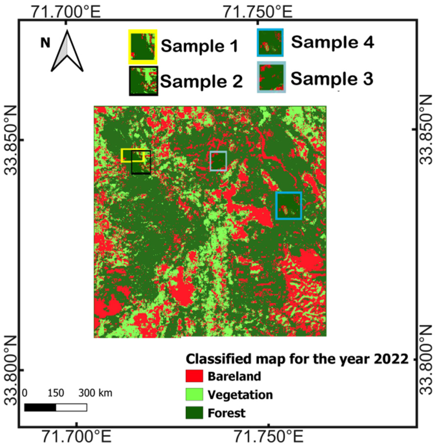
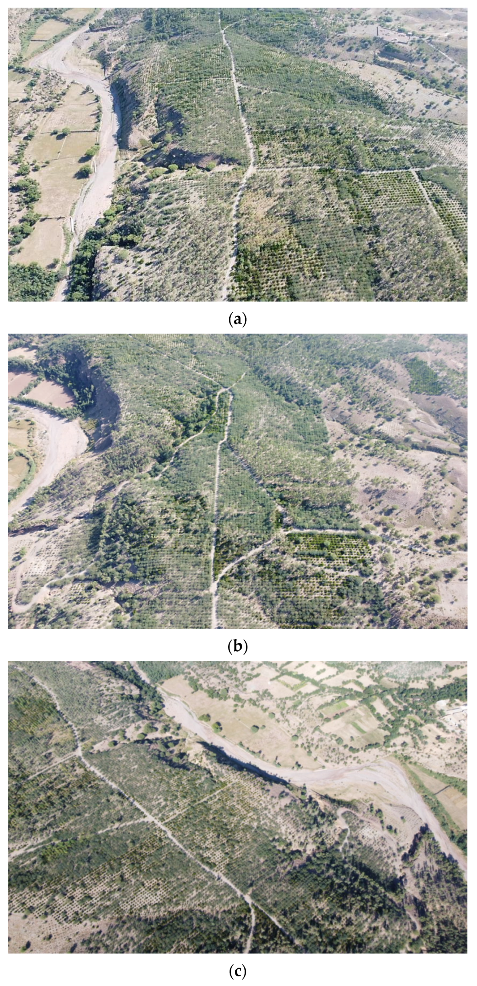
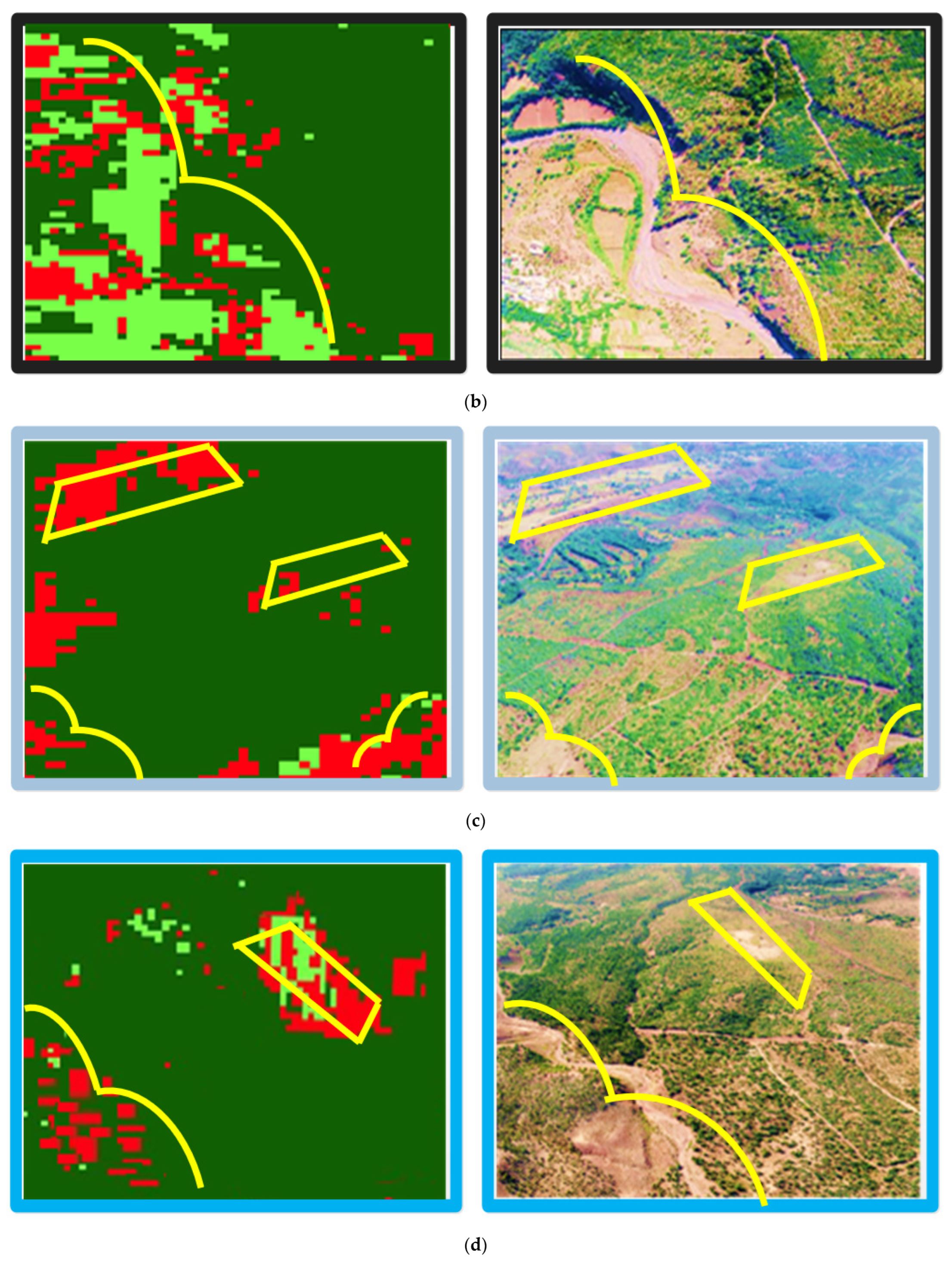
• Using an UAV drone, ground images are recorded for the classified image of the year 2022 and compared. A total of four sample areas are chosen within the total area of the classified image, and the coordinates of the sample areas are noted from the classified image and open street map. The ground images collected from the UAV are preprocessed and geo-referenced using MATLAB for its comparison with the classified image.

The rest of the paper is arranged as follows. In Section 2, materials and methods are discussed. Section 2 is further divided into subsections that include the details of the study area, image fusion method, classification, accuracy assessment and data recording using the UAV. Section 3 discusses the results and finally a conclusion is drawn based on the presented results.

2. Materials and Methods

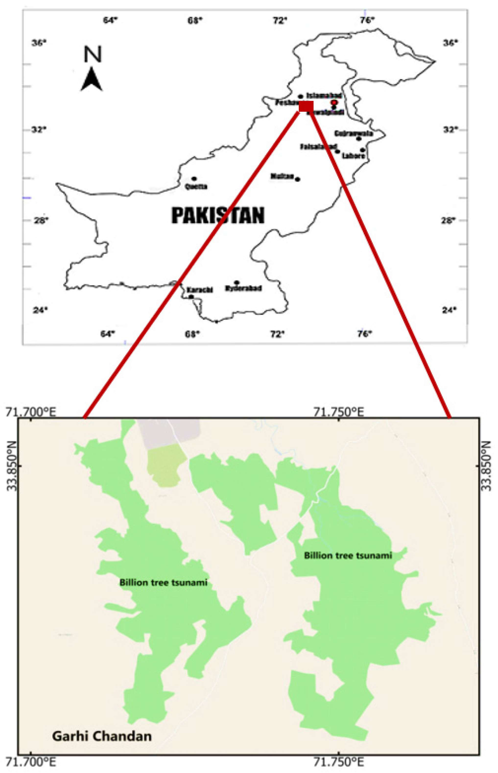
In this section, the details about the study area, image fusion method, classification, accuracy assessment and ground data sampling using an UAV are presented.

2.1. Study Area

Pakistan is geographically located between (23–38) degrees north in latitude and (61–78) degrees east in longitude. Ghari Chandan is situated nearby Peshawar, a city of Khyber Pakhtunkhwa province in Pakistan. Ghari Chandan is geographically located 33°50′0″ North and 71°42′0″ East. It is one of the sites in region 1 where the Billion Tree Tsunami plantation is already completed. The total area of our study location is 3141.6 hectares/31.42 million m².

Figure 1 shows the geographic map of Pakistan and the open street clipped map of our study area. It is observed from the open street map of the study area, that the forests are planted in two areas tagged as Billion Tree Tsunami, one to the left and the other to the right of the clipped map. In the study area, vegetation and forest growth is totally dependent on rain cycles and there are no canals or underground water available for irrigation purposes.

2.2. Image Fusion and Sharpening

In this work, the method presented in [49] is utilized to enhance the spatial resolution of all Sentinel-2 and Landsat 8 bands to 10 m. The proposed method uses optimization to estimate the projections into a low dimensional space. As given in [49], the cost function of the estimation method is represented as follows:

$$C(A,B)={\displaystyle \sum _{i=1}^{n}0.5\left|\right|{\varphi }_i-D_i{B}_i{a}_i\left|\right|}{}^2+{\displaystyle \sum _{j=1}^m{\delta }_j{\Omega }_w(z_j)}$$

(1)

The parameters given in Equation (1) and further concepts are discussed in [48,49]. In this work, the sharpened Sentinel-2 and Landsat 8 OLI images were downloaded using semi-automatic classification plugin (SCP) [45] and QGIS 3.16. A challenging task was how to link the downloaded data in the QGIS 3.16 to the sharpening algorithm written in MATLAB such that the geographical information of all bands was restored back after the image sharpening was performed. Figure 2 shows a flowchart that explains the whole process. As shown in the flowchart, the downloaded data for both Sentinel-2 and Landsat OLI satellites are imported to MATLAB. Prior to this step, raster world files are generated in QGIS and saved as. tfw files. Generally speaking, the raster in world file format will have the same geo spatial data for all bands of Sentinel-2 and Landsat 8 because the data is clipped to the same coordinated for both the satellites. After loading all the data onto the MATLAB working directory, built-in MATLAB functions are utilized to store the matrix and geospatial information. As explained earlier, ${\varphi }_i$ represents the structure array formed from the observed Sentinel-2 and Landsat 8 bands and as per the concepts presented in [49], the first 12 entries represent the Sentinel-2 bands except band 10, and the first seven bands of Landsat 8 are stored in the entries position 13–19. Further details are given in the flowchart shown in Figure 2.

2.3. Supervised Classification

In the introduction section, a detailed review about the three supervised classification, namely, the artificial neural network, decision tree and Random Forest Algorithm methods is presented. Artificial neural networks are computing systems inspired by the biological neural networks that constitute mathematical models derived from biological brains, which generate classification rules by recursively dividing data into increasingly homogeneous groups. The data is subdivided into smaller, more homogeneous groups (referred to as nodes) depending on predictive feature criteria. In comparison to the decision tree, the Random Forest Algorithm builds a “forest”, that is an ensemble of decision trees, usually trained with the “bagging/bootstrapping” method. The general idea of the bagging method is that a combination of learning models increases the overall result. A comparative analysis is shown in

Table 1. Comparison of ANN, decision tree and Random Forest Algorithm.

ANN	Decision Tree	Random Forest
The precision of the estimation depends on several factors such as increasing number of hidden layers, changing activation function and weights initialization	Suffers from over fitting if it is allowed to grow without control	Over fitting is addressed by taking the average of several decision trees or with most voting
Multi-layer neural networks are computationally costly and thus slow	Single tree is faster in computation	Multi decision tree requires relatively high computational power
Selection of hidden layers, weights and activation function is to be done manually or some other optimization techniques will be required	Fixed set of rules are required for prediction	Random buildup of decision trees and output is calculated based on average of several trees or majority voting

.

Based on the advantages offered by Random Forest Algorithm, this research work utilizes the Random Forest Algorithm for the forest classification. In this work, the SCP plugin of QGIS 3.16 is used for Random Forest classification of the data.

2.4. Accuracy Assessment

To calculate the total number of samples, the following relation is used [50,51]

$$S={\left({\displaystyle \sum _{i=1}^n{A}_i}\frac{{\delta }_i}{{\delta }_o}\right)}^2$$

(2)

where $S$ represents total number of samples to be designed for the classified image, $A_i$ represents the mapped area proportion to class $i$, ${\delta }_i$ shows the standard deviation of each class $i$ and ${\delta }_o$ represents the expected standard deviation to be achieved during accuracy assessment. In this work, ${\delta }_o$ = 0.01.

Now the samples for each class are calculated as follows [50,51]

$$S_i=\frac{\left(S{A}_i+\frac{S}{n}\right)}{2}$$

(3)

where $S_i$ represents the samples for each class and $n$ shows the number of classes. After sample design for each class, the rest of the processing is done using SCP plugin and QGIS 3.16 and the details are shown in Figure 3.

2.5. Ground Data Sampling Using UAV

In this work, a dji mavic mini 2 combo UAV was used to collect the ground data of the Billion Tree forests in our study area. The specifications of the UAV drone are given in the following link (https://www.dji.com/mini-2/specs) (accessed on 25 September 2022). Before collecting the ground data, a total of 4 sub sample areas were marked from within the classified image of the year 2022. Figure 4 shows the marked sub sample areas for which the ground data was collected using the UAV drone. As shown in Figure 4, the four sub sample areas are marked using yellow-, black-, light-sky-blue and dark-sky-blue-colored quadrilateral polygons. From QGIS, the clipped sub sample coordinates, length and width and respective centroids are tabulated in

Table 2. Sub sample coordinates in WGS 84/UTM zone 42N system.

	Sub Sample 1	Sub Sample 2	Sub Sample 3	Sub Sample 4
North	3,748,570	3,748,530	3,748,510	3,747,530
South	3,748,230	3,747,940	3,748,020	3,746,850
East	751,650	751,790	753,620	755,430
West	751,060	751,310	753,210	754,790
(L × W) m2	590 × 340	480 × 590	410 × 490	640 × 680
Centroid	295,170	240,295	205,245	320,340

.

The recorded coordinates for all sub samples are converted to decimal degree (DD). Since each sub sample represents quadrilateral polygons, so the corner point coordinates are marked with the help of a GPS device at the site location of each sub sample area. Then, for each rectangle polygon, the respective centroid can be easily marked on ground. The UAV can be vertically taken up from the centroid of each sub sample or it can record images when the camera and drone body is at an angle with respect to the ground plane of each sample. The geometric diagram interpretation for ground data collection using an UAV drone is shown in Figure 5a,b.

As given in Figure 5a,b, L and W represent the length and width of each sample, rs shows half of the length, r represents the radius of the imaginary circle viewed by the drone camera, h is the vertical height of the drone with respect to ground, hr, hm and hl show the sides of the triangles as perceived in the figures. The field of view (FOV) angle of the drone camera is represented as φ, the angular distance of the drone body from the centroid of the samples is measured by ρ, and α represents the angle between the ground axis and hm. As shown in the figure, the quadrilateral polygon has four corner points, P1, P2, P3, P4, and a center, C.

From the geometric interpretation of Figure 5a, the height of the drone can be calculated using the following expression, with α = 90 degrees.

$$h=\frac{r}{\tan (\raisebox{1ex}{$\varphi $}\!\left/ \!\raisebox{-1ex}{$2$}\right.)}$$

(4)

In Equation (4), $r$ is unknown, so we assume that $r=1.5\ast rs$ because for each sample $rs$ is known. From the geometric interpretation of Figure 5b, height of the drone can be calculated using the following expression with α > 90 degrees.

$$h=\frac{rm}{\tan (\rho -\raisebox{1ex}{$\varphi $}\!\left/ \!\raisebox{-1ex}{$2$}\right.)}$$

(5)

In Equation (5), $rm$ is unknown, so we calculate it from the current GPS location of the drone and the known centroid coordinate of each sample. After collection of ground data for all 4 samples, the following MATLAB algorithm is utilized for the images alignment and geo referencing. Please refer to Figure 6.

From (https://www.dji.com/mini-2/specs) (accessed on 25 September 2022), the drone can attain a maximum height of 4000 m above sea level, and it is equipped with Global Navigation Satellite System sensors such as GPS/GLONASS/GALILEO. The controllable range of the camera gimbals is between −90 to 0 degrees. The drone is equipped with a 12-megapixel camera with a total field of view (FOV) of 83 degrees. Using the mentioned parameters and Equation (5), the height and other parameters for the image collection are tabulated in

Table 3. Drone height and angle for ground data sampling.

	Sub Sample 1	Sub Sample 2	Sub Sample 3	Sub Sample 4
rs (m)	295	240	205	320
rm(m)	500	400	400	500
Φ (degrees)	83	83	83	83
ρ (degrees)-xb	−10	−10	−15	−15
ρ (degrees)-h	80	80	75	75
h (m)	628.5	502.8	604.3	755.4

. Please note that the angles are converted to radians. As shown in Table 3, the drone height is always within the range of 1 km from the ground level. Moreover, in Table 3, ρ (degrees)-xb represents the drone and camera angle with respect to the drone body x-axis, and ρ (degrees)-h shows the same angle with respect to the perpendicular line h.

For all samples, the images were recorded on 22 October 2022 with a camera zoom factor of 2, and the satellite images from 25 September 2022 were acquired for the year. Figure 7a–c shows the acquired clipped images. These images are preprocessed in MATLAB.

3. Results

In the section below, the results are presented with the following subsections.

3.1. Image Sharpening

The left side of Figure 8a shows the original Sentinel-2 band 1 (60 m), and the right side of Figure 8a shows the sharpened image representing band 1 (10 m) using the proposed method. Similarly, Figure 8b shows the original Landsat 8 band 1 (30 m) and the sharpened Landsat 8 band 1 (10 m). From Figure 8 and by visually comparing the 60 m bands sharpened to a 10 m spatial resolution, all blur pixels are sharpened, and the pixels of the obtained sharpened images are clear enough. Generally, it is hard to compare the original and sharpened bands visually, thus performance indicators reported in [49] are calculated. The performance indicators include relative dimensionless global error (ERGAS), root mean square error (RMSE), spectral angular mapper (SAM), universal quality index (UQI), signal-to-reconstruction error (SRE) and structural similarity index measure (SSIM).

Table 4. ERGAS, RMSE and SAM scores.

	ERGAS	RMSE	SAM
20 m	7.1	0.001	7.05
30 m	1.23	0	1.23
60 m	0.47	0	0

and

Table 5. SRE, SSIM and UIQI scores.

	SRE	SSIM	UIQI
Band 5-S (20 m)	13.12	0.88	0.50
Band 6-S (20 m)	14.14	0.89	0.50
Band 7-S (20 m)	14.27	0.89	0.55
Band 8A-S (20 m)	14.19	0.89	0.55
Band 11-S(20 m)	14.37	0.86	0.47
Band 12-S(20 m)	13.89	0.82	0.45
Band 8-L(20 m)	13.45	0.92	0.68
Average	13.918	0.8786	0.5286
Band 1-L (30 m)	11.01	0.89	0.62
Band 2-L (30 m)	11.31	0.86	0.69
Band 3-L (30 m)	13.33	0.87	0.69
Band 4-L (30 m)	13.43	0.87	0.67
Band 5-L (30 m)	15.05	0.85	0.68
Band 6-L (30 m)	14.46	0.81	0.66
Band 7-L (30 m)	12.37	0.81	0.60
Average	12.99	0.8514	0.6586
Band 1-S (60 m)	15.57	0.91	0.72
Band 9-S (60 m)	15.86	0.85	0.68
Average	15.71	0.88	0.70

shows the performance indicator of the sharpened bands calculated for 20 m, 30 m and 60 m data. As observed from the tabulated data, the calculated ERGAS, SAM and RMSE scores for 20 m, 30 m and 60 m bands are well within the range of values calculated in [49]. From Table 4 the estimated ERGAS scores of 0.47, 1.23 and 7.1 were recorded for 20 m, 30 m and 60 m bands, respectively. A lower ERGAS score represents that the distortion in the fused image is low. The lowest ERGAS score of 0.47 was recorded for the 60 m band, which means that it has the lowest distortion. Similarly, Table 5 shows the magnitude of SRE, SSIM and UIQI scores for 20 m, 30 m and 60 m bands and their respective averages. The comparison of the tabulated scores in Table 5 with the data presented in [49] show that all the scores are in an acceptable range. From Table 5, the average estimated UIQI scores of 0.52, 0.65 and 0.70 were recorded for 20 m, 30 m and 60 m bands, respectively. Here it is worth mentioning that UIQI index 1 means that the image quality is perfect with less distortion. A score of 0.70, which is close to 1, was recorded for 60 m. From Table 4, the estimated SAM scores of 7.05, 1.23, 0 were recorded for 20 m, 30 m bands, respectively. Here it is worth mentioning that a SAM score of zero means that the image has a small spectral angle distortion.

3.2. Image Classification

Figure 9 shows the classified data for the years 2016, 2018, 2020 and 2022. Since the Billion Trees plantation drive was initiated in 2014 and continued onwards, a two-year gap was chosen for the data collection. Moreover, the study area of Ghari Chandan has no abundant underground water for irrigation purposes and the growth of the plants is totally dependent on rainfall.

From Figure 9a–d, the classification reports are generated from the classified data and the results are tabulated in

Table 6. Parameters of classified images.

Year 2022
Class	Pixel Sum	Percentage %	Area (×106 m2)
1. Forest	177,669	56.553	17.7669
2. Bare land	79,766	25.390	7.97660
3. Vegetation	56,725	18.157	5.67250
Year 2020
Class	Pixel sum	Percentage %	Area (×106 m2)
1. Forest	113,858	36.502	11.4675
2. Bare land	158,051	50.670	15.9186
3. Vegetation	402,979	12.827	4.0298
Year 2018
Class	Pixel sum	Percentage %	Area (×106 m2)
1. Forest	69,337	22.070	6.9337
2. Bare land	180,561	57.474	18.0561
3. Vegetation	64,262	20.455	6.4262
Year 2016
Class	Pixel sum	Percentage %	Area (×106 m2)
1. Forest	30,047	9.564	3.0047
2. Bare land	227,790	72.507	22.7790
3. Vegetation	56,323	17.928	5.6323

. From the tabulated data for the years 2016, 2018, 2020 and 2022, the total classified area in each case is 3141.6 hectares/31.416 million m². The forest areas for the years 2016, 2018, 2020 and 2022 are estimated as 9.564%, 22.070%, 36.502% and 56.553%, respectively. From the estimated percent areas for all four years, it is concluded that for equal time intervals (2-year period), nearly proportional increases in the forest areas are observed. Moreover, the vegetation percent areas for the years 2016, 2018 and 2022 are almost in the same range. However, for the year 2020, a decreased classified area is observed for the vegetation class. This may be due to the classification accuracy errors and less rainy seasons in the study area.

3.3. Accuracy Assessment

Table 7. Samples stratification for the classified data of the year 2022.

Year 2022
Class	$\mathit{S}{\mathit{\delta }}_{\mathit{i}}$	$\mathit{S}\mathbf{/}\mathit{n}$	Average
1. Forest	147	87	117
2. Bare land	66	86	76
3. Vegetation	47	87	67
Total	260	260	260

shows the sample stratification for each class. In this work, a total of three classes are considered i.e., $n=3$. In addition, the standard deviation for each class was chosen as follows: ${\delta }_1=0.1,{\delta }_2=0.2,{\delta }_3=0.3$. From Equations (2) and (3), the parameters defined above, and the percentage of area proportion for each class given in Table 6 for the year 2022, the total number of samples calculated are tabulated as $S$ = 260. Table 7 shows the sample’s stratification for the classified data of the year 2022 for each class. From

Table 8. Accuracy assessment parameters for the classified data of the year 2022.

Area Based Error Matrix for the Classified Data of the Year 2022
Classified	Reference
		1. Forest	2. Bare land	3. Vegetation
	1. Forest	0.5442	0.0142	0.0071
	2. Bare land	0.0092	0.2354	0.0092
	3. Vegetation	0.0118	0.0196	0.1492
	Total % Area	0.5652	0.2692	0.1655
	Standard Error	0.0131	0.0126	0.0142
	PA [%]	96.28	87.42	90.12
	UA [%]	96.22	92.72	82.60
	Kappa hat	0.91	0.90	0.79
	Estimated area (×106 m2)	17.7564	8.4600	5.1995

, the accuracy assessment parameters for the classified data of the year 2022, the overall classification accuracy [%] is recorded as 92.87% with an overall Kappa hat classification = 0.8777. This proves that the classified area is mapped to the ground truths by a very high percentage. Similarly, using Equations (2) and (3), the defined standard deviation of each class $i$ and expected standard deviation and the percentage of area proportion for each class given in Table 6 for the year 2020, the total number of samples calculated are as follows: $S$ = 309.

Table 9. Samples stratification for the classified data of the year 2020.

Year 2020
Class	$\mathit{S}{\mathit{\delta }}_{\mathit{i}}$	$\mathit{S}\mathbf{/}\mathit{n}$	Average
1. Forest	113	103	108
2. Bare land	157	103	130
3. Vegetation	39	103	71
Total	309	309	309

shows the sample’s stratification for the classified data of the year 2020 for each class.

Table 10. Accuracy assessment parameters for the classified data of the year 2020.

Area Based Error Matrix for the Classified Data of the Year 2020
Classified	Reference
		1. Forest	2. Bare land	3. Vegetation
	1. Forest	0.2022	0.0612	0.0071
	2. Bare land	0.1622	0.1214	0.0090
	3. Vegetation	0.0237	0.3110	0.1022
	Total % Area	0.3881	0.4936	0.1183
	Standard Error	0.0231	0.0131	0.0099
	PA [%]	90.12	89.14	87.12
	UA [%]	88.34	82.10	82.60
	Kappa hat	0.85	0.80	0.77
	Estimated area (×106 m2)	12.1929	15.5065	3.7165

shows the accuracy assessment parameters such as area error matrix, overall accuracy, standard error and the Kappa hat score for the classified data of the year 2020. As tabulated in Table 10, an overall classification accuracy [%] of 90.79% with an overall Kappa hat classification of 0.8611 is achieved.

Using Equations (2) and (3), the defined standard deviation of each class $i$ and the expected standard deviation and the percentage of area proportion for each class given in Table 6 for the year 2018, the total number of samples calculated are as follows: $S$ = 393.

Table 11. Samples stratification for the classified data of the year 2018.

Year 2018
Class	$\mathit{S}{\mathit{\delta }}_{\mathit{i}}$	$\mathit{S}\mathbf{/}\mathit{n}$	Average
1. Forest	87	131	109
2. Bare land	225	131	178
3. Vegetation	81	131	106
Total	393	393	393

shows the samples stratification for the classified data of the year 2018 for each class.

Table 12. Accuracy assessment parameters for the classified data of the year 2018.

Area Based Error Matrix for the Classified Data of the Year 2018
Classified	Reference
		1. Forest	2. Bare land	3. Vegetation
	1. Forest	0.0097	0.5392	0.0258
	2. Bare land	0.0096	0.0116	0.1833
	3. Vegetation	0.1802	0.0202	0.0202
	Total % Area	0.1995	0.5711	0.2294
	Standard Error	0.0108	0.0129	0.0124
	PA [%]	90.31	94.42	79.91
	UA [%]	81.65	93.82	89.62
	Kappa hat	0.77	0.85	0.86
	Estimated area (×106 m2)	6.2689	17.9401	7.2069

shows the accuracy assessment parameters such as standard error in the area of each class, user and producer accuracies, Kappa hat and the estimated area. From the tabulated data, an overall accuracy [%] of 90.27% with a Kappa hat classification score of 0.8326 is observed. Moreover, the standard errors in area for each class are in the acceptable range. For the last dataset of the year 2016, using Equations (2) and (3), and the defined standard deviation of each class $i$ with expected standard deviation and the percentage of area proportion for each class given in Table 6, the total number of samples calculated are as follows: $S$ = 432.

Table 13. Samples stratification for the classified data of the year 2016.

Year 2016
Class	$\mathit{S}{\mathit{\delta }}_{\mathit{i}}$	$\mathit{S}\mathbf{/}\mathit{n}$	Average
1. Forest	40	144	92
2. Bare land	314	144	229
3. Vegetation	78	144	111
Total	432	432	432

shows the samples stratification for the classified data of the year 2016 for each class.

Table 14. Accuracy assessment parameters for the classified data of the year 2016.

Area Based Error Matrix for the Classified Data of the Year 2016
Classified	Reference
		1. Forest	2. Bare land	3. Vegetation
	1. Forest	0.0348	0.6776	0.0127
	2. Bare land	0.0000	0.0097	0.1695
	3. Vegetation	0.0830	0.0126	0.0001
	Total % Area	0.1179	0.6999	0.1823
	Standard Error	0.0108	0.0130	0.0074
	PA [%]	70.44	96.81	93.05
	UA [%]	86.81	93.44	94.59
	Kappa hat	0.85	0.78	0.93
	Estimated area (×106 m2)	3.7026	21.9875	5.7257

shows the accuracy assessment parameters such as standard error in the area of each class, user and producer accuracies, Kappa hat and the estimated area. From the tabulated data, an overall accuracy [%] of 93.02% with a Kappa hat classification = 0.8444 is achieved. The accuracy assessment scores are in the acceptable range, so it is concluded that the classified image is in perfect agreement with the true values.

3.4. Change Map of the Study Area for the Years 2016–2022

In this subsection, a change map for the period 2016–2022 is calculated and shown in Figure 10. From the obtained change map, the total area of the cross classes and % changes in the area of each cross class are given in Figure 11. From the presented results, it is obvious that during the time interval 2016–2022, approximately 41% of the bare land classified for the data of the year 2016 has been mapped onto forest class by the year 2022. Similarly, from Figure 11, it is shown that a 21% change in the area of the bare land class is observed during the time interval 2016–2022. This is due the fact that the study area had some natural plant growth and deforestation had occurred due to natural effects or human interventions. Except from the two above-discussed cross classes, the remaining cross classes have fewer changes in the areas.

3.5. Ground Data Matching

Figure 12a–d shows the classified sub area samples and the actual data recorded using a UAV drone. Figure 12a shows the classified sub area sample 1 and the corresponding ground data image recorded using the UAV. By comparing the two images, it is concluded that the classified sample area is in good agreement with the actual image. However, a portion of classified sample area represents vegetation class, and it cannot be matched to the real image. This is due the fact that the classification accuracy has some errors, as discussed in the accuracy assessment subsection.

Similarly, Figure 12b shows the classified sub area sample 2 and the corresponding ground data image recorded using the UAV. By comparing the two images, it is concluded that the classified sample area is in good agreement with the actual image. However, a portion of classified sample area below the tagged line represents a mix of vegetation and bare land classes. Figure 12c shows the classified sub area sample 3 and the corresponding ground data image recorded using UAV. By comparing the two images, it is concluded that the classified sample area is in good agreement with the actual image. However, the upper portion of the real image contains some portions that represent the bare land class; whereas, the classified sub area sample 3 does not include such a class. Figure 12d shows the classified sub area sample 4 and the corresponding ground data image recorded using UAV. By comparing the two images, it is concluded that the classified sample area is also in good agreement with the actual image. However, the right middle portion of the classified image contains a bare land class; whereas, the actual image does not include such a landscape.

4. Discussions

In order to verify the ground truth about the plantation drive done as a result of the Billion Tree Tsunami project initiation by the government of Pakistan in Khyber Pakhtunkhwa, province (https://en.wikipedia.org/wiki/Billion_Tree_Tsunami) (accessed on 25 September 2022), this research work utilized the multispectral satellite images freely available from Sentinel and Landsat programs and classified the data. Before classification, the data obtained from the two satellites were fused using a model-based approach [49] and all bands for both satellites were sharpened to a spatial resolution of 10.

For image sharpening, the performance indicators are tabulated in Table 4 and Table 5. From the tabulated data, the average scores of the signal-to-reconstruction error (SRE), structural similarity index measure (SSIM) and universal quality index (UQI) for 20 m bands are calculated as 13.918, 0.8786 and 0.5286. Similarly for 30 m bands, the average SRE, SSIM and UQI scores are noted as 12.99, 0.8514 and 0.6586, respectively. For 60 m bands, the average calculated scores for SRE, SSIM and UQI are 15.71, 0.88 and 0.70 respectively. Moreover, from Table 4, the calculated scores for the relative dimensionless global error (ERGAS), root mean square error (RMSE) and spectral angular mapper (SAM) for 20 m, 30 m and 60 m bands are in good agreement with the scores presented in [49]. From the above discussions, it is concluded that the image sharpening results for all bands have attained a high accuracy. It can also be verified that objective 2 defined in the introduction section is fulfilled. In order to fulfill objectives 1 and 3, the classified images and the accuracy assessment indicators are presented in Figure 8, Figure 9, Figure 10 and Figure 11 and Table 6, Table 7, Table 8, Table 9, Table 10, Table 11, Table 12, Table 13 and Table 14. From analysis of the tabulated data in the above tables, for the year 2022, an overall classification accuracy [%] was recorded as 92.87% with an overall Kappa hat classification = 0.8777. Similarly, for the classified data of the year 2020, an overall classification accuracy [%] of 90.79% with an overall Kappa hat classification of 0.8611 was achieved. For the year 2018, an overall accuracy [%] of 90.27% with a Kappa hat classification score of 0.8326 is observed and for the year 2016, an overall accuracy [%] of 93.02% with a Kappa hat classification = 0.8444 was achieved. These results show that the classified data is in a perfect agreement with the reference data. Moreover, the scores for the standard error (SE) in the area, user and producer accuracies are in the acceptable ranges. Lastly, a change map was created from the classified data of the years 2016–2022. The results are presented in Figure 9, Figure 10 and Figure 11. From the presented results, a 41% change in area of bare land from the classified data of the year 2016 is mapped as forests in the year 2022. This shows the authentication of objectives 1 and 3. The last objective of this study was to verify the classified data with the ground truths and it was fulfilled by recording the ground samples of four regions using an UAV. The results are given in Figure 12 and the classified samples are in good agreement with the ground data.

The image sharpening technique presented in [49] was utilized in this research work; however, an interface algorithm was developed that automatically copies the data from a designated folder of QGIS, extracts the geospatial raster data for each band and lastly combines the sharpened images with the geospatial raster data extracted in step 2 so that the final images are ready for classification in QGIS. This is a way in which the method presented in [49] was automated and the QGIS data was linked to MATLAB in a convenient way. As reported in [52], very limited studies have been conducted for land cover and forest mapping in Pakistan during the time period of 1993–2021 and only 73 peer-reviewed articles were published during the above-mentioned period of time. Moreover, from the data tabulated in [52], the images acquired from Landsat 2, 3, 5, 7, 8 were mostly utilized for forest mapping; whereas, in this research work, an image fusion technique was utilized to combine the Landsat 8 OLI and Sentinel-2 multispectral images for sharpening all the bands to 10 m spatial resolution. Moreover, the average overall accuracies for forest mapping in Pakistan are reported to range between 82 and 95%; however, in most cases, ground data is not considered. In our reported results, the same has been considered and verified. Overall, the research results presented in this work fulfil all the shortcomings (theoretical and experimental) pointed out in [52].

5. Conclusions and Future Work

This article has presented a supervised classification of the Billion Tree Tsunami forest plantation drive initiated by the government of Pakistan in Khyber Pakhtunkhwa province using a Random Forest Algorithm. For our study area, images were acquired from Sentinel-2 and Landsat 8 satellites and a model-based method was utilized for the sharpening of all bands to a 10 m spatial resolution. The sharpened data of four years was classified and an accuracy assessment was done for each dataset. From the results and discussion section, it has been concluded that the accuracy assessment scores including overall accuracy, Kappa hat and the standard area errors are in the acceptable range so the classified data is in good agreement with the reference data. Finally, the classified data of the year 2022 was compared with the real data acquired by an UAV, and both the datasets show satisfactory agreement with each other. This work has a potential future extension for developing algorithm-level autonomy for the UAV to virtually mark the sample areas using a GPS device and record the ground images. Similarly, the same techniques can be extended to classify and analyze all regions of the Billion Tree Tsunami project.

References

1. Hansen, M.C.; DeFries, R.; Townshend, J.R.; Sohlberg, R. Global land cover classification at 1 km spatial resolution using a classification tree approach. Int. J. Remote Sens. 2000, 21, 1331–1364. [Google Scholar] [CrossRef]
2. Hosonuma, N.; Herold, M.; De Sy, V.; De Fries, R.S.; Brockhaus, M.; Verchot, L.; Angelsen, A.; Romijn, E. An assessment of deforestation and forest degradation drivers in developing countries. Environ. Res. Lett. 2012, 7, 44009. [Google Scholar] [CrossRef]
3. Phiri, D.; Morgenroth, J.; Xu, C. Long-term land cover change in Zambia: An assessment of driving factors. Sci. Total Environ. 2019, 697, 134206. [Google Scholar] [CrossRef] [PubMed]
4. Jucker, T.; Caspersen, J.; Chave, J.; Antin, C.; Barbier, N.; Bongers, F.; Dalponte, M.; van Ewijk, K.Y.; Forrester, D.I.; Haeni, M.J.G.C.B. Allometric equations for integrating remote sensing imagery into forest monitoring programmes. Glob. Chang. Biol. 2017, 23, 177–190. [Google Scholar] [CrossRef] [PubMed] [Green Version]
5. Haack, B.N. Landsat: A tool for development. World Dev. 1982, 10, 899–909. [Google Scholar] [CrossRef]
6. Turner, W.; Rondinini, C.; Pettorelli, N.; Mora, B.; Leidner, A.K.; Szantoi, Z.; Buchanan, G.; Dech, S.; Dwyer, J.; Herold, M. Free and open-access satellite data are key to biodiversity conservation. Biol. Conserv. 2015, 182, 173–176. [Google Scholar] [CrossRef] [Green Version]
7. Denize, J.; Hubert-Moy, L.; Corgne, S.; Betbeder, J.; Pottier, E. Identification of winter land use in temperate agricultural landscapes based on Sentinel-1 and 2 Times-Series. In Proceedings of the IGARSS 2018-2018, IEEE International Geoscience and Remote Sensing Symposium, Valencia, Spain, 22–27 July 2018; pp. 8271–8274. [Google Scholar]
8. Immitzer, M.; Vuolo, F.; Atzberger, C. First Experience with Sentinel-2 data for crop and tree species classifications in Central Europe. Remote Sens. 2016, 8, 166. [Google Scholar] [CrossRef]
9. ESA. Sentinel-2 Missions-Sentinel Online; ESA: Paris, France, 2014. [Google Scholar]
10. Lu, D.; Weng, G. A survey of image classification methods and techniques for improving classification performance. Int. J. Remote Sens. 2004, 28, 823–870. [Google Scholar] [CrossRef]
11. Landgrebe, D.A. Signal Theory Methods in Multispectral Remote Sensing; John Wiley: Hoboken, NJ, USA, 2003. [Google Scholar]
12. Chen, K.S.; Tzeno, Y.C.; Chen, C.F.; Kao, W.I. Land cover classification of multispectral imagery using dynamic learning neural network. Photogramm. Eng. Remote Sens. 1995, 81, 403–408. [Google Scholar]
13. Foody, G.M. Supervised classification by MLP and RBN neural networks with and without an exhaustive defined set of classes. Int. J. Remote Sens. 2004, 5, 3091–3104. [Google Scholar] [CrossRef]
14. Huang, W.Y.; Lippmann, R.P. Neural Net and Traditional Classifiers. In Neural Information Processing Systems; American Institute of Physics: College Park, MD, USA, 1988; pp. 387–396. [Google Scholar]
15. Eberlein, S.J.; Yates, G.; Majani, E. Hierarchical multisensor analysis for robotic exploration. In Proceedings of the SPIE 1388, Mobile Robots, Advances in Intelligent Robotics Systems, Boston, MA, USA, 4–9 November 1990; Volume 578, pp. 578–586. [Google Scholar]
16. Cleeremans, A.; Servan-Schreiber, D.; McClelland, J.L. Finite State Automata and Simple Recurrent Networks. Neural Comput. 1989, 1, 372–381. [Google Scholar] [CrossRef]
17. Decatur, S.E. Application of neural networks to terrain classification. In Proceedings of the International Joint Conference on Neural Networks, Washington, DC, USA, 18–22 June 1989; Volume 1, pp. 283–288. [Google Scholar]
18. Kulkarni, A.D.; Lulla, K. Fuzzy Neural Network Models for Supervised Classification: Multispectral Image Analysis. Geocarto Int. 1999, 14, 42–51. [Google Scholar] [CrossRef]
19. Laprade, R.H. Split-and-merge segmentation of aerial photographs. Comput. Vis. Graph. Image Process. 1988, 44, 77–86. [Google Scholar] [CrossRef]
20. Hathaway, R.J.; Bezdek, J.C. Recent convergence results for the fuzzy c-means clustering algorithms. J. Classification 1988, 5, 237–247. [Google Scholar] [CrossRef]
21. Pal, S.K.; De, R.K.; Basak, J. Unsupervised Feature Evaluation: A Neuro-Fuzzy Approach. IEEE Trans. Neural Netw. 2000, 11, 366–376. [Google Scholar] [CrossRef] [Green Version]
22. Kulkarni, A.; McCaslin, S. Knowledge Discovery From Multispectral Satellite Images. IEEE Geosci. Remote Sens. Lett. 2004, 1, 246–250. [Google Scholar] [CrossRef]
23. Mountrakis, G.; Im, J.; Ogole, C. Support vector machines in remote sensing: A Review. Int. J. Photogramm. Remote Sens. 2011, 60, 247–259. [Google Scholar] [CrossRef]
24. Mantero, P.; Moser, G.; Serpico, S.B. Partially supervised classification of remote sensing images through–SVM-based probability density estimation. IEEE Trans. Geosci. Remote Sens. 2005, 43, 559–570. [Google Scholar] [CrossRef]
25. Mitra, P.; Shankar, B.U.; Pal, S.K. Segmentation of multispectral remote sensing images using active support vector machines. Pattern Recognit. Lett. 2004, 25, 1067–1074. [Google Scholar] [CrossRef]
26. Hansen, R.M.; Dubayah, R.; DeFries, R. Classification trees: An alternative to traditional land cover classifiers. Int. J. Remote Sens. 1990, 17, 1075–1081. [Google Scholar] [CrossRef]
27. Ghose, M.K.; Pradhan, R.; Ghose, S. Decision tree classification of remotely sensed satellite data using spectral separability matrix. Int. J. Adv. Comput. Sci. Appl. 2010, 1, 93–101. [Google Scholar]
28. Breiman, L. Random Forests. Mach. Learn. 2001, 45, 5–32. [Google Scholar] [CrossRef]
29. Gislason, P.O.; Benediktsson, J.A.; Sveinsson, J.R. Random forest for land cover classification. Pattern Recognit. Lett. 2006, 27, 294–300. [Google Scholar] [CrossRef]
30. Geetha, V.; Punitha, A.; Abarna, M.; Akshaya, M.; Illakiya, S.; Janani, A.P. An Effective Crop Prediction Using Random Forest Algorithm. In Proceedings of the 2020 International Conference on System, Computation, Automation and Networking (ICSCAN), Pondicherry, India, 3–4 July 2020; pp. 1–5. [Google Scholar] [CrossRef]
31. Pelletier, C.; Valero, S.; Inglada, J.; Champion, N.; Dedieu, G. Assessing the robustness of Random Forests to map land cover with high resolution satellite image time series over large areas. Remote Sens. Environ. 2016, 187, 156–168. [Google Scholar] [CrossRef]
32. Belgiu, M.; Drăgu¸t, L. Random forest in remote sensing: A review of applications and future directions. ISPRS J. Photogramm. Remote Sens. 2016, 114, 24–31. [Google Scholar] [CrossRef]
33. Pallagani, V.; Khandelwal, V.; Chandra, B.; Udutalapally, V.; Das, D.; Mohanty, S.P. dCrop: A Deep-Learning Based Framework for Accurate Prediction of Diseases of Crops in Smart Agriculture. In Proceedings of the 2019 IEEE International Symposium on Smart Electronic Systems (iSES) (Formerly iNiS), Rourkela, India, 16–18 December 2019; pp. 29–33. [Google Scholar] [CrossRef]
34. Rodriguez-Galiano, V.F.; Ghimire, B.; Rogan, J.; Chica-Olmo, M.; Rigol-Sanchez, J.P. An assessment of the effectiveness of a random forest classifier for land-cover classification. ISPRS J. Photogramm. Remote Sens. 2012, 67, 93–104. [Google Scholar] [CrossRef]
35. Ma, L.; Li, M.; Ma, X.; Cheng, L.; Du, P.; Liu, Y. A review of supervised object-based land-cover image classification. ISPRS J. Photogramm. Remote Sens. 2017, 130, 277–2933. [Google Scholar] [CrossRef]
36. Malenovský, Z.; Rott, H.; Cihlar, J.; Schaepman, M.E.; García-Santos, G.; Fernandes, R.; Berger, M. Sentinels for science: Potential of Sentinel-1, -2, and -3 missions for scientific observations of ocean, cryosphere, and land. Remote Sens. Environ. 2012, 120, 91–101. [Google Scholar] [CrossRef]
37. Korhonen, L.; Packalen, P.; Rautiainen, M. Comparison of Sentinel-2 and Landsat 8 in the estimation of boreal forest canopy cover and leaf area index. Remote Sens. Environ. 2017, 195, 259–274. [Google Scholar] [CrossRef]
38. Pesaresi, M.; Corbane, C.; Julea, A.; Florczyk, A.J.; Syrris, V.; Soille, P. Assessment of the added-value of Sentinel-2 for detecting built-up areas. Remote Sens. 2016, 8, 299. [Google Scholar] [CrossRef]
39. Drusch, M.; Del Bello, U.; Carlier, S.; Colin, O.; Fernandez, V.; Gascon, F.; Hoersch, B.; Isola, C.; Laberinti, P.; Martimort, P.; et al. Sentinel-2: ESA’s Optical High-Resolution Mission for GMES Operational Services. Remote Sens. Environ. 2012, 120, 25–36. [Google Scholar] [CrossRef]
40. USGS EROS Archive—Sentinel-2—Comparison of Sentinel-2 and Landsat. Available online: https://www.usgs.gov/centers/eros/science/usgs-eros-archive-sentinel-2-comparison-sentinel-2-and-landsat (accessed on 26 October 2022).
41. Drakonakis, G.I.; Tsagkatakis, G.; Fotiadou, K.; Tsakalides, P. OmbriaNet—Supervised Flood Mapping via Convolutional Neural Networks Using Multitemporal Sentinel-1 and Sentinel-2 Data Fusion. IEEE J. Sel. Top. Appl. Earth Obs. Remote Sens. 2022, 15, 2341–2356. [Google Scholar] [CrossRef]
42. Hafner, S.; Nascetti, A.; Azizpour, H.; Ban, Y. Sentinel-1 and Sentinel-2 Data Fusion for Urban Change Detection Using a Dual Stream U-Net. IEEE Geosci. Remote Sens. Lett. 2022, 19, 1–5. [Google Scholar] [CrossRef]
43. Chen, Y.; Bruzzone, L. Self-Supervised SAR-Optical Data Fusion of Sentinel-1/-2 Images. IEEE Trans. Geosci. Remote Sens. 2022, 60, 1–11. [Google Scholar] [CrossRef]
44. Li, Z.; Zhang, H.K.; Roy, D.P.; Yan, L.; Huang, H. Sharpening the Sentinel-2 10 and 20 m Bands to Planetscope-0 3 m Resolution. Remote Sens. 2020, 12, 2406. [Google Scholar] [CrossRef]
45. Clerici, N.; Calderon, C.A.V.; Posada, J.M. Fusion of Sentinel-1A and Sentinel-2A data for land cover mapping: A case study in the lower Magdalena region, Colombia. J. Maps 2017, 13, 718–726. [Google Scholar] [CrossRef] [Green Version]
46. Ma, Y.; Chen, H.; Zhao, G.; Wang, Z.; Wang, D. Spectral Index Fusion for Salinized Soil Salinity Inversion Using Sentinel-2A and UAV Images in a Coastal Area. IEEE Access 2020, 8, 159595–159608. [Google Scholar] [CrossRef]
47. Ao, Z.; Sun, Y.; Xin, Q. Constructing 10 m NDVI Time Series from Landsat 8 and Sentinel 2 Images Using Convolutional Neural Networks. IEEE Geosci. Remote Sens. Lett. 2020, 18, 1461–1465. [Google Scholar] [CrossRef]
48. Shao, Z.; Cai, J.; Fu, P.; Hu, L.; Lui, T. Deep learning-based fusion of Landsat-8 and Sentinel-2 images for a harmonized surface reflectance product. Remote Sens. Environ. 2019, 235, 111425. [Google Scholar] [CrossRef]
49. Sigurdsson, J.; Armannsson, S.E.; Ulfarsson, M.O.; Sveinsson, J.R. Fusing Sentinel-2 and Landsat 8 Satellite Images Using a Model-Based Method. Remote Sens. 2022, 14, 3224. [Google Scholar] [CrossRef]
50. Olofsson, P.; Foody, G.M.; Herold, M.; Stehman, S.V.; Woodcock, C.E.; Wulder, M.A. Good practices for estimating area and assessing accuracy of land change. Remote Sens. Environ. 2014, 148, 42–57. [Google Scholar] [CrossRef]
51. Congedo, Luca, Semi-Automatic Classification Plugin: A Python tool for the download and processing of remote sensing images in QGIS. J. Open Source Softw. 2021, 6, 3172. [CrossRef]
52. Ahmad, A.; Ahmad, S.R.; Gilani, H.; Tariq, A.; Zhao, N.; Aslam, R.W.; Mumtaz, F. A Synthesis of Spatial Forest Assessment Studies Using Remote Sensing Data and Techniques in Pakistan. Forests 2021, 12, 1211. [Google Scholar] [CrossRef]
Figure 1. Geographic map of Pakistan and the study area encircled in red rectangle.
Ijgi 12 00009 g001
Figure 2. Flowchart explaining how to link QGIS and MATLAB for image sharpening.
Ijgi 12 00009 g002
Figure 3. Flow chart representing accuracy assessment of the classified data.
Ijgi 12 00009 g003
Figure 4. Sub area samples marked on classified image for UAV data collection.
Ijgi 12 00009 g004
Figure 5. Sub area sample ground image collection using UAV (a) when UAV is vertical about point C and camera is vertically down (b) when UAV and camera are at an angle ρ from point C.
Ijgi 12 00009 g005aIjgi 12 00009 g005b
Figure 6. Flowchart explaining how to collect and process ground data using an UAV.
Ijgi 12 00009 g006
Figure 7. Real images acquired by UAV for ground data samples (a) sample 1 (b) sample 2 (c) sample 3 (d) sample 4.
Ijgi 12 00009 g007aIjgi 12 00009 g007b
Figure 8. (a) Left: Sentinel-2 band 1 original, Right: Sentinel-2 band-1 sharpened image. (b) Left: Landsat 8 band-1 original, Right: Landsat 8 band-1 sharpened image.
Ijgi 12 00009 g008
Figure 9. Classified images for the years (a) 2016, (b) 2018, (c) 2020, (d) 2022.
Ijgi 12 00009 g009
Figure 10. Change map for the years 2016–2022.
Ijgi 12 00009 g010
Figure 11. Cross classes % area calculated from the change map 2016–2022.
Ijgi 12 00009 g011
Figure 12. (a) Left: classified sub area sample 1, Right: Actual image of sub area sample 1, (b) Left: classified sub area sample 2, Right: Actual image of sub area sample 2, (c) Left: classified sub area sample 3, Right: Actual image of sub area sample 3, (d) Left: classified sub area sample 4, Right: Actual image of sub area sample 4.
Ijgi 12 00009 g012aIjgi 12 00009 g012b