Article

Incorporating Spatial Autocorrelation in Machine Learning Models Using Spatial Lag and Eigenvector Spatial Filtering Features

1
Department of Geo-Information Processing, Faculty of Geoinformation Science and Earth Observation (ITC), University of Twente, 7514 AE Enschede, The Netherlands
2
Department of Geography and Regional Research, University of Vienna, Universitätsstraße 7, 1010 Vienna, Austria
*
Author to whom correspondence should be addressed.
ISPRS Int. J. Geo-Inf. 2022, 11(4), 242; https://doi.org/10.3390/ijgi11040242
Submission received: 12 January 2022 / Revised: 22 March 2022 / Accepted: 2 April 2022 / Published: 7 April 2022

Abstract

:
Applications of machine-learning-based approaches in the geosciences have witnessed a substantial increase over the past few years. Here we present an approach that accounts for spatial autocorrelation by introducing spatial features to the models. In particular, we explore two types of spatial features, namely spatial lag and eigenvector spatial filtering (ESF). These features are used within the widely used random forest (RF) method, and their effect is illustrated on two public datasets of varying sizes (Meuse and California housing datasets). The least absolute shrinkage and selection operator (LASSO) is used to determine the best subset of spatial features, and nested cross-validation is used for hyper-parameter tuning and performance evaluation. We utilize Moran’s I and local indicators of spatial association (LISA) to assess how spatial autocorrelation is captured at both global and local scales. Our results show that RF models combined with either spatial lag or ESF features yield lower errors (up to 33% different) and reduce the global spatial autocorrelation of the residuals (up to 95% decrease in Moran’s I) compared to the RF model with no spatial features. The local autocorrelation patterns of the residuals are weakened as well. Compared to benchmark geographically weighted regression (GWR) models, the RF models with spatial features yielded more accurate models with similar levels of global and local autocorrelation in the prediction residuals. This study reveals the effectiveness of spatial features in capturing spatial autocorrelation and provides a generic machine-learning modelling workflow for spatial prediction.

1. Introduction

The volume of data generated in recent years is increasing tremendously and a large proportion of big data is geospatial (e.g., remote-sensing imagery, GPS trajectories, weather measurements) [1]. Geospatial big data bears the same features as normal big data, such as big volume, high velocity, and high variety, and provides new opportunities to uncover previously unknown insights into our world. However, one of the associated challenges with spatial big data lies in developing new methods to handle and analyze complex datasets where traditional approaches may fail [2].
Machine learning (ML) methods allow computers to learn from data and can extract information and identify structures from large and high-dimensional datasets [3]. With the advent of geospatial big data, ML has been universally employed in geoscientific research such as land cover classification [4,5], landslide susceptibility [6], climate change studies [7], and atmospheric dynamics [8]. One of the main uses of ML on geospatial data is spatial prediction in which a model is built using training samples to predict unknown values at specific locations [9,10].
In contrast with ML methods, which are generic and can be applied to various datasets, spatial methods specifically aim to analyze geospatial data. Spatial methods are built upon the first law of geography, which states that “everything is related to everything else, but near things are more related than distant things” [11,12,13]. Such characteristics of spatial phenomena imply the underlying spatial dependence or spatial autocorrelation (SAC). The presence of this spatial relationship violates the assumption of identical and independent distribution (i.i.d.) upon which many non-spatial statistical methods are predicated. Hence, spatial methods distinguish themselves in explicitly dealing with spatial dependence or SAC.
Spatial autoregressive [14] and geographically weighted regression (GWR) [15] are two commonly used spatial methods for spatial prediction. Models based on spatial autoregressive methods can be configured differently depending on where SAC is introduced [14,16]. For instance, the spatial lag model assumes SAC in the response variable and the spatial error model specifies spatial dependencies in the error term. GWR represents a localized linear regression method to build models that capture spatial heterogeneity by estimating spatially varying parameters [17]. Another research field that deals with spatial autocorrelation is geostatistics. Kriging covers a family of methods to create models that interpolate spatially autocorrelated variables. It captures SAC by determining the spatial covariance of samples using a variogram model. However, all these methods mentioned above suffer from divergent drawbacks. Spatial autoregressive and GWR mainly focus on linear relationships. Kriging usually requires assumptions about spatial distribution (e.g., second-order stationary), which may be unrealistic in practice [18]. Additionally, it is difficult to scale kriging and GWR for big spatial computation [19,20].
ML is generally accurate, flexible, and scalable for analyzing complex data but does not automatically recognize spatial context. Therefore, the direct application of ML to geospatial data without accounting for the potential spatial autocorrelation could lead to biased outcomes [21,22,23,24].
Present research concerning the incorporation of ML and spatial analysis is still relatively limited or scarce. Existing approaches could be roughly categorized in four directions: inclusion of spatial features in original algorithms [22,25,26], hybrid models with geostatistics [27,28,29,30], cluster-based methods in which cluster analysis on independent variables is introduced as a preprocessing procedure [31], and other algorithms exclusively designed for spatial problems such as spatial predictive clustering trees (PCTs) [32] and SpaceGAN [33].
The aforementioned four directions manifest diverse advantages and unique research values. In this paper, we investigate the inclusion of spatial features. In ML, features are equivalent to the notion of explanatory variables in statistics. Thus, spatial features refer to variables that reflect geographical connectivity and spatial relations between observations, potentially accounting for SAC [22]. Feature engineering represents a crucial process in ML that aims to extract and formulate suitable features for the expected model. Multiple options exist to specify spatial features: Euclidean distance fields (EDF), which include buffer distances (distance to sampling locations) and coordinates [25], spatial lag based on a definition of a neighborhood [26,34,35]. The major advantage of including spatial features over exclusively spatial algorithms is that this does not require direct modification of the original methods, thus reviving non-spatial ML in geographical contexts and maintaining the variety of models that are already established scientifically.
The goal of this study is to explore the role of spatial features in a generic ML prediction context. Specifically, our objectives are to (a) present a workflow for the engineering and evaluation of spatial features, and (b) assess whether such features capture SAC and improve prediction performance.

2. Related Work

Research on the combination of spatial features and ML is emerging in these years. Behrens et al. [25] introduced a spatial modeling framework with generic EDF as additional spatial covariates. They combined EDF with other commonly used environmental covariates in the case of digital soil mapping. Six ML methods were chosen to compare against a reference obtained from regression kriging. The inclusion of EDF enables ML to infer spatial autocorrelation when predicting at new locations without an additional step to correct residuals using kriging. Hengl et al. [22] presented a random forest framework for spatial prediction (RFsp) that accounts for spatial effects by using multiple distance-based features including EDF. They evaluated the effectiveness of buffer distances on five environmental datasets. Their results demonstrate that RFsp can produce similar predictions to ordinary kriging and regression kriging, while RFsp does not demand strict assumptions about distribution and stationarity. However, these authors also pointed out that it is difficult to derive buffer distance variables for large datasets.
Apart from explicit distance-based features, studies on the incorporation of other spatial features and ML mainly concentrate on spatial lags. Li et al. [26] proposed a geo-intelligent deep learning approach in which spatially and temporally lagged PM2.5 terms were combined with satellite-derived and socioeconomic indicators in a deep belief network model. Their analysis proved that including spatial lag as a representation of geographical relations significantly improves the accuracy of the estimations. Kiely and Bastian [34] incorporated spatial lag features into multiple ML algorithms to predict real estate sales. The comparison results indicated an enhanced predictive performance of spatially aware models over non-spatial counterparts. In the work of Zhu et al. [35], the authors followed the same technique as Li et al. [26] to include lagged features in several ML algorithms. The modified algorithms showed great improvement in terms of accuracy when reconstructing the surface air temperature across China.
In summary, current research confronts limitations as well as opportunities for further research. First, buffer distance features cannot fully satisfy the requirements for all spatial problems, especially the ones involving large amounts of data samples. Second, spatial lag features were constructed and examined with distance-based computations but they can also be engineered via the specification of spatial weight matrix and neighbor-based computations. Third, eigenvector spatial filtering features have not been developed and examined in the context of spatial ML prediction.

3. Methods

Figure 1 illustrates our modelling and analytical procedure, which is further detailed in the following subsections. Section 3.1 describes the data on which the experiments are based. Section 3.2 explains how spatial features are incorporated in ML. We propose two types of features: the spatial lag features (configured via a spatial weight matrix and neighbor-based computations) and the ESF features. In Section 3.3 we explain the training and evaluation of the models. The scripts used to engineer the spatial features, build the models, as well as to evaluate the results are available in a public repository (please refer to Data Availability Statement).

3.1. Data Sources

Two public spatial datasets with different properties are used in this study to test the usability of the proposed modelling.

3.1.1. Meuse River Dataset

Meuse is a classical spatial dataset in geostatistics that consists of samples collected in a flood plain of the river Meuse in the Netherlands. Hengl et al. [22] used Meuse dataset for one of the experiments where distance-based spatial features were introduced in ML models. It is internally integrated with several R packages such as “gstat” [36] and “sp” [37]. Furthermore, due to its publicity and availability, it has been used for other spatial analytical tasks such as spatial clustering [38] and spatial autoregressive models [39]. We use 153 samples for which four heavy metal concentrations were being measured. Geographical locations are also included, together with soil and landscape variables. Details about the data variables are described in Table 1. Interpolation of zinc concentration is usually the main focus of this dataset. Flooding frequency and distance to the river can be considered as covariates in regression kriging to predict zinc concentration with the assumption that the river is the main source of zinc. Figure 2a shows the distribution of zinc concentrations. Each category has an approximately equal number of observations that are determined by quantiles. A higher concentration of zinc is observed along the western riverbank.

3.1.2. California Housing Dataset

This dataset contains 20,640 observations of California housing prices based on 1990 California census data. Each row represents a census block group or district (the smallest geographical unit for which the U.S. Census Bureau publishes sample data). It was originally used by Pace and Barry [40] to build spatial autoregressive models, and it is considered a standard example dataset with spatial autocorrelation [33]. Median house price, location of the samples, and six other explanatory variables are described in Table 2. The price values are classified by quantiles in Figure 2b. Coastal regions usually hold higher house prices, especially for districts around metropolitan cities such as San Francisco and Los Angeles. Because different districts are populated with varying numbers of households, the total number of rooms or bedrooms (original pre-processed variables) were divided by the number of households in this study to obtain the average variable. Here the task is to create a model that predicts housing prices.

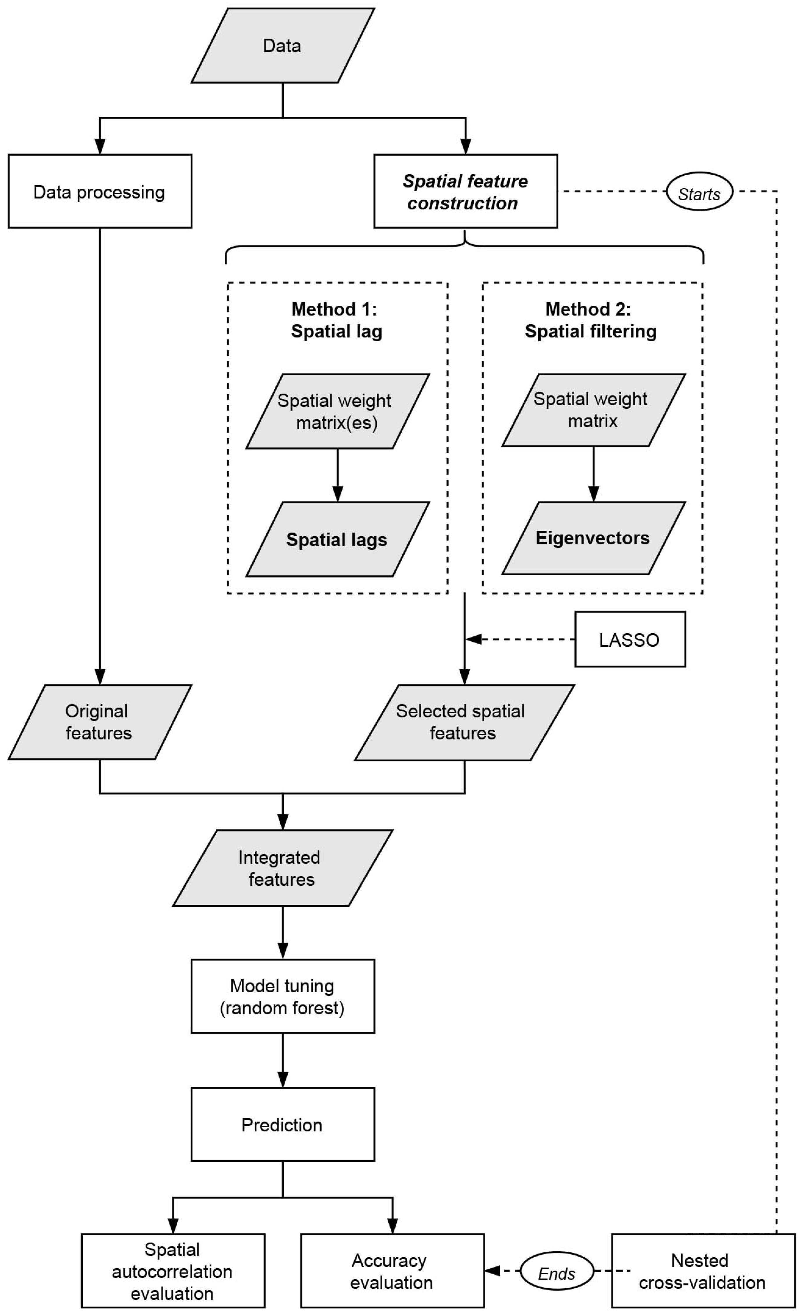
3.2. Construction and Processing of Spatial Features

3.2.1. Spatial Lag Features

The spatial lag features capture the spatial autocorrelation of the dependent variables (y) in surrounding areas. The spatial lag of location i is calculated as the weighted sum of values from location i to j:
L a g i = j w i j y j
A spatial weight matrix (wij) is necessary to construct lag features. In principle, the construction of such a spatial weight matrix involves two procedures: definition of a neighborhood, and calculation of spatial weights. The neighborhood determines which locations are linked (i to j) and the weights determine the strength of links. The weights can be either determined by binary settings or calculated through distance-based functions such as inverse distance and kernel functions. Different specifications of the matrix represent varying spatial structures. However, there does not exist a consensus on the choice of a spatial weight matrix [41]. In this study, the binary setting of a k-nearest neighbor is utilized as it provides a convenient interface to construct the spatial weight matrix by changing the value of parameter k. K-nearest neighbor also introduces an adaptive connectivity configuration, in which the number of neighbors is constant but the distance range between neighbors is not. The weight matrix is row-standardized such that lag features represent the average of surrounding values. Thus, the weight values are:
w i j = { 1 / k ,   i f   i   a n d   j   a r e   n e i g h b o r s 0 ,                                     o t h e r w i s e  
Many efforts have been invested in selecting an appropriate spatial matrix for spatial autoregressive regression. Rather than one single matrix, different spatial weight matrices can be used to include multiple spatial lags in one regression model aiming to capture different types of dependence [42]. We follow a similar approach: for the Meuse dataset, an increasing sequence of 5, 10, 15 is used for parameter k (thus creating three spatial weights matrices) to generate the spatial lag features. As the California housing dataset covers a larger area, 5, 10, 15, 50 nearest neighbors are employed (thus creating four spatial weights matrices) to generate the spatial lag features. This is a data-driven approach to empirically configure the k values and include different possibilities of the neighbors. These values as well as the number of matrices can be changed depending on the characteristics of the data and problem at hand.

3.2.2. Eigenvector Spatial Filtering

Eigenvector spatial filtering (ESF) is a regression technique proposed by Getis and Griffith [43] to enhance the model results in the presence of spatial dependence. This idea is originated from Moran’s I, in which the spatial weight matrix is used to capture the spatial covariations.
ESF decomposition is conducted on the matrix
( I 11 T / n ) W ( I 11 T / n )  
where I is an n-by-n identity matrix, 1 is an n-by-1 vector of ones, and W is the spatial weight matrix as defined by Getis and Griffith [43]. The extracted eigenvectors furnish the underlying latent map patterns [44].
The transformation of the spatial matrix occurs to make it positive semi-definite. Orthogonal and uncorrelated eigenvectors are used as synthetic variables in the regression problem to enable the model to account for spatial autocorrelation [43,45,46,47].
Eigen-decomposition, which is essential for ESF, is computationally intensive for large samples. To improve computing efficiency, Murakami and Griffith [20] proposed to approximate the first L (L << n) eigenvectors using the Nyström extension [48]. They employed k-means clustering on the spatial coordinates and regarded the cluster centers as the knots for the Nyström extension. The authors advised calculating at least 200 eigenvectors to effectively remove positive spatial autocorrelation with small approximation errors and to capture spatial characteristics successfully.
ESF is often used as an exploratory technique, but it can also be used to predict values at unknown locations by using the Nyström approximation. However, this approximation technique cannot deal with negative spatial dependence and is only limited to spatial weight matrices that are based on positive semidefinite kernels such as Gaussian or exponential kernels [20].
In this study, we adopt the common exponential kernel from Murakami and Griffith [20] because these authors demonstrated its usability in large datasets. The elements of the spatial weight matrix are calculated as:
w i j = exp ( d i j r )
where dij is the distance between location i and j, and r is given by the maximum length in the minimum spanning tree that connects all the samples. The exponential kernel can be substituted with any kernel function to meet the requirements of other problems as long as the kernel is semidefinite [20]. Due to the sample size and computational concern of eigen-decomposition, only the first 200 eigenvectors are approximated for California housing data. For the Meuse dataset, the exact eigenvalues are calculated without approximation.

3.3. Machine Learning and Benchmarking Models

This section explains the implementation of the machine learning (ML) models using Random Forest (Section 3.3.1) as well as that of the benchmark model based on Geographically Weighted Regression (Section 3.3.2). The implementation includes hyperparameter tuning and feature selection for the ML models and parameter tuning for the benchmark model. The modelling procedures were implemented for the two data sets (Meuse and California) and to create four kinds of models: (i) non-spatial models purely based on the original features available for each dataset, (ii) spatial lag models, (iii) ESF models, and (iv) benchmark models.

3.3.1. Random Forest

Random forest (RF) is used in this study for its general accuracy and successful applications in diverse geoscientific problems [28,35,49]. RF has also been used as a framework recently to integrate distance variables in spatial prediction [22]. During the training phase, we tuned the number of features used in node splitting (commonly known as “mtry “). The number of trees is kept at a moderate size of 200 trees for a balance between computational efficiency and predictive stability.
We implemented a least absolute shrinkage and selection operator (LASSO) feature selection approach to minimize the number of spatial features used to train the models as well as to get a better sense of their usefulness. LASSO is a regularization method developed by Tibshirani [50] that is widely used ML for feature selection. It sets an L1 constraint on linear regression and penalizes the coefficients by shrinking a part of them to exactly zero. A hyper-parameter λ ≥ 0 controls the strength of L1 penalty in LASSO, which can be tuned by cross-validation. Features with non-zero coefficients are preserved in the final model. The largest value of lambda such that the error is within one standard error of the minimum is often used for the selected model [51].
Although RF can help combat the problem of the curse of dimensionality [52], numerous studies use feature selection methods in combination with RF [53]. Empirical results have shown that applying dimensionality reduction techniques with RF may yield nearly the same predictive performance [54] or it can even increase it [55].
Furthermore, we foresee that the proposed modelling workflow could be implemented with alternative algorithms for which dimensionality reduction may be needed when the number of dimensions is too large for the sample size [56,57,58]. Except for the original shape of the data, a high number of dimensions may also result after a feature engineering process. For instance, ESF may introduce 200 or more additional eigenvector features. For a dataset with a smaller size, the number of features may exceed the number of observations. Regarding spatial lag, any number of features could be added if that is desired. The LASSO approach retains the representative features (ESF or Spatial Lag) and excludes the unnecessary ones, which is beneficial when applying and testing models in terms of model interpretability, complexity, and time efficiency. Although LASSO has been chosen because it is a common approach and it is computationally efficient, it is also a linear model. Hence, features with non-linear relationships, which can be detected by RF, may be excluded. Its application should be used selectively and by considering the data and the problem at hand. Furthermore, alternative feature selection methods may be considered, such as RF mean decrease in accuracy, RF Recursive Feature Elimination, VSURF, SVM Recursive Feature Elimination, and Correlation-based Feature Selection [59,60].

3.3.2. Geographically Weighted Regression

To benchmark our proposed modelling approach, we use both a traditional “a-spatial” RF and a classical spatial statistical model, namely a Geographically Weighted Regression (GWR). GWR has been successfully used to model various geospatial application domains, including the housing market [61], health [62], tourism [63], sharing economy [64], policy-making [65], and crime [66].
GWR returns local parameter estimates for each relationship between dependent and independent variables at each location and can thus produce a parameter surface across the study region [67]. The method explores local linear relationships and is designed for ratio covariates. Therefore, in the implementation of the GWR model for the Meuse data we excluded the variables ffreq, soil, landuse, and lime as opposed to the RF models. For the California models, the same set of covariates was used.
The models were implemented by the MGWR module in Python spatial analysis library (PySAL) developed by Oshan et al. [68]. The authors suggest optimizing a model fit criterion to select the bandwidth when there is no theoretical guide to manually specify it. The fit criterion that we employed for the optimization of the bandwidth is the corrected Akaike information criterion (AICc). Default settings were employed for the kernel function (i.e., “bi-square”) and the kernel type (i.e., adaptive nearest neighbor). The bi-square kernel function is the default behavior because it avoids a potential issue of all observations retaining some weight and also because it indicates the distance above which the parameters have no influence [68]. In addition, the adaptive kernel type ensures that there will be no calibration issues in the sparsely populated regions of the study area.

3.4. Performance Evaluation

To retrieve a more objective performance evaluation of our approach, we adopted the idea of nested cross-validation (CV). The fundamental idea of CV is to separate the dataset into different parts: training and testing. This ensures that the information of the test subset does not leak during the training process. The result is given by CV and therefore represents an objective estimate of how the model will generalize on unseen data. With nested CV the optimal hyper-parameters of inner folds are tested in an outer fold, in an iterative and nested manner [69]. Nested CV is a suitable approach to evaluate the generalization abilities of a model that prevents bias in estimates [70], also known as “double cross” [71].
Two layers of k-fold cross-validation are included in the nested CV. The outer CV serves for estimation while the inner CV takes care of other procedures such as hyper-parameter tuning (in our RF implementation this is the selected feature). Inner folds are obtained by splitting the outer training folds. The hyper-parameters are determined by inner CV, then the optimal values are used to fit a model on the outer training set. The generalized performance reported by nested CV is the average over the outer testing folds.
The nested CV process used in this study is further summarized as follows:
(a)
Split the dataset into K outer folds.
(b)
For each outer fold k = 1, 2, …, K: outer loop for model evaluation:
  • Take fold k as outer testing set outer-test; take the remaining folds as outer training set outer-train.
  • Split the outer-train into L inner folds.
  • For each inner fold l = 1, 2, …, L: inner loop for hyper-parameter tuning:
    i.
    Take fold l as inner testing set inner-test and the remaining as inner-train.
    ii.
    Calculate spatial features on the inner-train.
    iii.
    Perform cross-validated LASSO on inner-train with spatial features, and determine the lambda λ with “one-standard-error” rule; Select the spatial features with non-zero coefficients.
    iv.
    For each hyper-parameter candidate, fit a model on the inner-train with the combined feature set.
    v.
    Calculate the selected spatial features on the inner-test.
    vi.
    Evaluate the model on inner-test with the assessment metric.
  • For each hyper-parameter candidate, average the assessment metric values across L folds and choose the best hyper-parameter. In our experiments, the hyperparameter that was tested was mtry.
  • Calculate spatial features on the outer-train.
  • Perform cross-validated LASSO on outer-train with spatial features, and determine the lambda λ with “one-standard-error” rule. Select the spatial features with non-zero coefficients.
  • Train a model with the best hyper-parameter on the outer-train.
  • Calculate the selected spatial features on the outer-test.
  • Evaluate the model on outer-test with the assessment metric.
(c)
Average the metric values over K folds, and report the generalized performance.
The lag features for testing samples (steps 3. V and 8) were derived from a rebuilt spatial weight matrix, which describes the spatial relations between this single testing location and all the training samples. Eigenvector features of testing samples were approximated by Nyström extension value (steps 3. V and 8). For the LASSO procedure we employed a 10-fold CV (steps 3. III and 6).
The evaluation metric that we use (steps 3. VI and 9) is the root mean square error (RMSE). The nested CV process was implemented in 5 outer folds (K) and 3 inner folds (L). Thus, 5 models were tested and derived the average test error. This error indicates the generalization ability of a model; in other words, how the final model would perform on potential unseen data.
For the benchmark GWR models, data were split into 80% train data and 20% test data (20% yields an equal size to an outer CV fold). Then, the RMSE of the predicted values from the test data were calculated too. Furthermore, we calculated as training error the RMSE when all data are fitted into a model (repeated to all model types: non-spatial, spatial lag, ESF, and GWR). This error indicates the fitting ability of a model; in other words, how well the model fits this specific dataset.

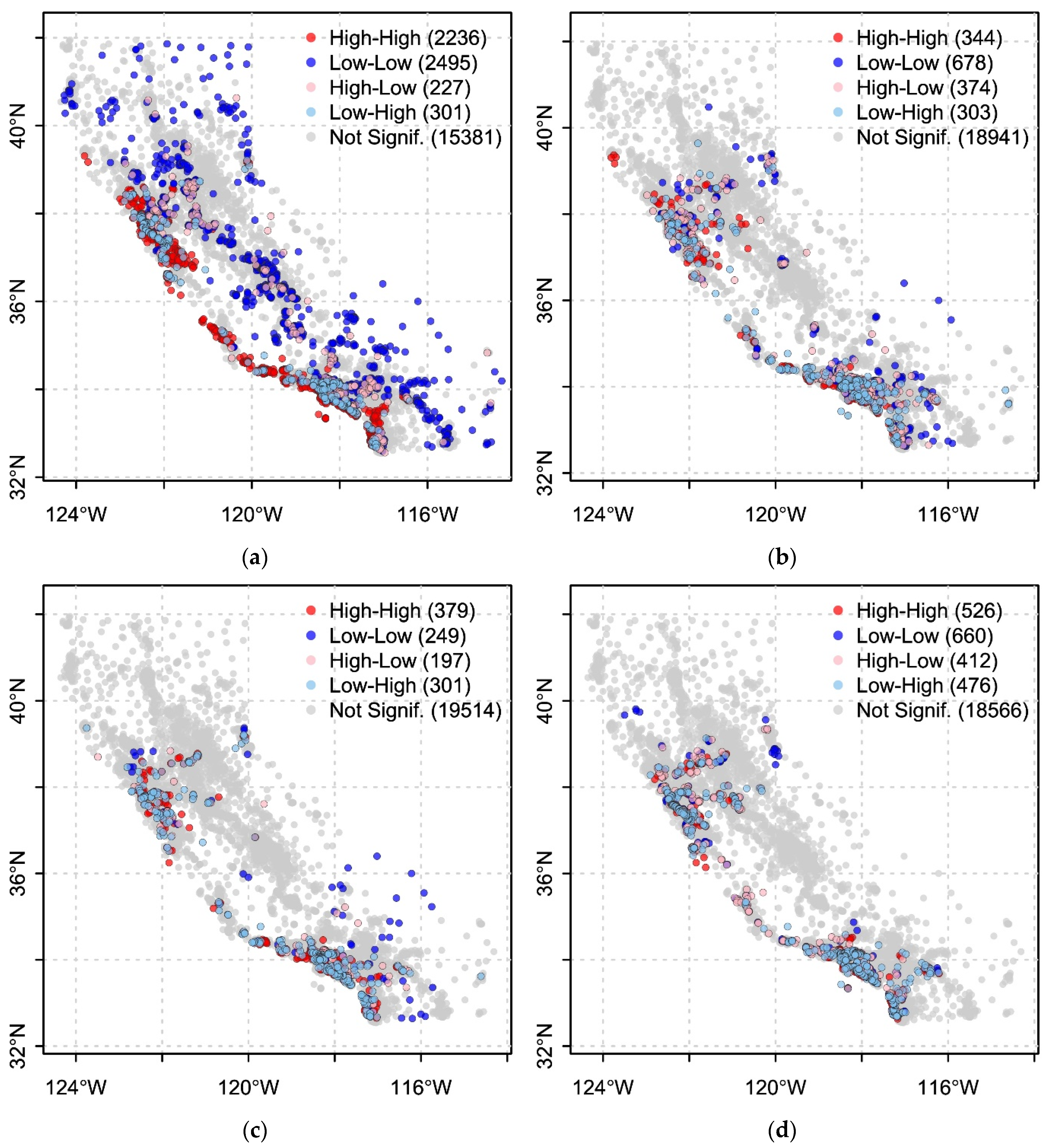
3.5. Spatial Autocorrelation Evaluation

When data-driven models are directly applied to spatial data without considering spatial effects, residuals might remain spatially autocorrelated [25,48,69]. Preferably the SAC of residuals should be minimized or even eliminated, which would imply that the model performs similarly in space and that there are minimal (or no) subregions with strong patterns of over- or underestimated values. The Moran’s I metric can be used for this purpose to detect and quantify global spatial autocorrelation in residuals. Moran’s I varies from −1 to +1. A positive value indicates positive spatial autocorrelation and a negative value indicates otherwise. Zero value means no spatial autocorrelation.
Furthermore, local indicators of spatial association (LISA) clusters of residuals are utilized to examine the existence of local patterns. LISA were built from the decomposition of Moran’s I and introduced by Anselin [72] to assess local spatial autocorrelation. Four groups with significant local spatial autocorrelation (High-High, Low-Low, Low-High, High-Low) can be captured by LISA. High-High (HH) and Low-Low (LL) indicate clustering of high and low values, respectively. Low-High (LH) denotes low values surrounded by high values, and the High-Low (HL) group denotes high values surrounded by low values.
Both the global Moran’s I and LISA were tested under Monte Carlo simulation [72] and were derived from nearest neighbor spatial weights matrices based on k = 5 nearest neighbors. These statistics were implemented in a model that was trained using a standard 5-fold CV on the entire dataset. The CV was used to derive the optimal mtry and then LASSO was used to select the spatial features. The final model (i.e., model fit all data) was trained using the subset of features and the best mtry.

4. Results

Section 4.1 describes the specification of the models, such as which spatial features were constructed and selected for the models as well as the values of the optimized parameters. In Section 4.2, we analyze the impact of the explanatory variables and how this varies by each model. Section 4.3 presents the performance evaluation results derived by RMSE calculations, while Section 4.4 presents the spatial autocorrelation evaluation results derived by Moran’s I and LISA statistics (maps depicting the distribution of models’ residuals can be found in the Supplementary Materials).

4.1. Specifications of the Models

The models and their specifications are shown in Table 3. For the GWR models, the bandwidth was optimized at 50 m for the Meuse data and 80 m for the California data. Although RF Meuse models are trained on different feature sets (e.g., non-spatial has only original features or lag model has fewer features than the ESF model), the best “mtry” value is equal to 5 for all of them. For the RF California models, the “mtry” is higher (i.e., 6) for the spatial models and lower (i.e., 2) for the non-spatial model.
Regarding the spatial lag features of the Meuse data, they were constructed with the number of nearest neighbors equal to 5, 10, 15, respectively, while the selected one was the lag_k5. For the California data, lags of more k-nearest-neighbors were used and the selected ones were these for 5, 10, and 15 neighbors.
The Meuse dataset contains fewer than 200 observations, so the eigenvalues of the weight matrix were not approximated but rather precisely calculated. The ESF features were then selected by LASSO. Eigenvector features are indicated by “ev” and a number. “ev1” represents the eigenvector corresponding to the largest eigenvalues, and likewise, the numbers follow. However, since the California dataset contains more than 20,000 observations, it is impractical and unnecessary to calculate eigenvalues of the full spatial weight matrix. Thus, 200 eigenvalues were approximated from the exponential kernel matrix. Due to the content limits, the selected ESF features are not shown in Table 3 but were in total 77 features.

4.2. Importance of Explanatory Variables

In this section, we look at the influence that each explanatory variable (i.e., features) has on the tested models (Table 4). For the RF models, the relative feature importance of the final model is extracted. Relative feature importance is obtained by scaling the original values to 0–100%. For the benchmark GWR models, different estimate parameters are calculated in each location. To compare the impact of the covariates, we present the mean absolute coefficient derived from the standardized coefficients at each location. Figure 3 shows the bedroomsAvg and population coefficients for the California dataset, as well as the elevation and distance coefficients for the Meuse dataset. We see that the coefficient values vary spatially and the patterns also are different between the covariates. This indicates spatial heterogeneity in both datasets. Furthermore, we calculated the number of observations (i.e., locations) for which the coefficient is significant. Following the approach by da Silva and Fotheringham [73], significance is calculated with corrected t-tests for testing the significance of local parameter estimates to avoid excessive false positives.
For the Meuse GWR model, the variable om (organic matter) has the highest mean absolute standardized coefficient (i.e., 0.43) but is also insignificant for more than half of the locations. For the Meuse RF models, distance to the river and elevation are the first and respectively the second most influential features for all models. Interestingly, for the GWR models, although coefficients’ values may vary across locations due to spatial heterogeneity they are also significant everywhere. This indicates how important these two features are for the models regardless of considering or not spatial properties (e.g., autocorrelation or heterogeneity). Spatial autocorrelation is also important in modelling Meuse data because the inclusion of spatial features such as lag_k5 or ev34 displaces other features (e.g., om or ffreq) further down regarding their relative importance. Nevertheless, spatial features appear to be less influential compared to distance and elevation.
Regarding the California models, the results are quite different. First, spatial features are largely predominant in the spatial lag and ESF models, which indicates that spatial autocorrelation is important for the house-price models. Secondly, in the GWR models, for a large number of locations non-spatial features are not significant, which indicates a larger diversity in “where” in the study area these explanatory variables are important (at least compared to the Meuse data). Furthermore, in some cases, these are the features with high-to-moderate coefficients in the models (e.g., roomsAvg and income). For instance, income coefficient values are insignificant for 28.16% of the samples (5814 locations). This could explain why in the non-spatial model, income is ranked first regarding its feature importance.

4.3. Performance Evaluation—RMSE Error

In Table 5 we see the training and test errors derived from RMSE values across the models. In both datasets, models with spatial features yielded the lowest test errors. That is the ESF model Meuse with a test error of 171.82 and the Spatial Lag model California with a test error of 44034.95. GWR models have the second-lowest errors. Concerning the highest errors, for the Meuse data, the test error is the highest in the non-spatial model (191.04), but for the California data, the ESF model has the highest error (68158.81).
The training errors show that the spatial features models fit the data better than the non-spatial models. However, they also show how largely lower the errors are compared to the test errors. To a certain degree this is because the training error is derived from models (model fit all data) of larger sample size, but also because with the inclusion of more features, RF tends to overfit the data, and thus when applied to unseen data the error will be higher. The training errors of the GWR models are much higher than those of the RF models. Nevertheless, they also have closer values to the values of the test errors. Thus, when using GWR to train a model to be used for out-of-sample predictions, the evaluation of the trained model will be more realistic than that of an RF model.
When comparing non-spatial with spatial RF models, the test error in three out of the four comparisons (i.e., 1. spatial lag Meuse vs. non-spatial Meuse, 2. ESF Meuse vs. non-spatial Meuse, 3. spatial lag California vs. non-spatial California, 4. ESF California vs. non-spatial California), shows that the models with spatial features are more accurate because the error has lower values ranging from 4% up to 33%. The exception to this is the ESF California model with a 3% higher test error compared to the error of non-spatial California model. Similarly, incorporating either spatial lag or ESF substantially lowers the training error (ranging from 5% up to 40% of lower values).

4.4. Spatial Autocorrelation Evaluation—Lobal and Local Moran’s I

Both the global and local autocorrelation of the residuals is significantly improved in the spatial RF models and the GWR models compared to the non-spatial models. In Table 6, we see the Moran’s I values and the number of insignificant LISA clusters of the residuals. Maps that depict the four LISA groupings including the insignificant values are shown in Figure 4 (for the Meuse data) and Figure 5 (for the California data). The maps show the clustering regions of overestimated values (HH), underestimated values (LL), as well as cluster outliers (HL and LH). The integer in parentheses refers to the number of observations within each category.
Regarding the number of insignificant LISA clusters, the GWR model has the highest number for the Meuse data (139) and the ESF model has the highest number for the California data (19,514). In an ideal model, there would be no significant LISA clusters at all. This would imply at first that there are no other spatial properties that are not captured by the models, and secondly, it could validate that the performance evaluation done by a global statistic, such as RMSE, is robust and does not vary greatly within the study area.
Similar observations to the LISA clusters can be made for the Moran’s I values that show statistically significant clustering patterns for both non-spatial models (i.e., 0.2 for the Meuse data and 0.42 for the California data). The Meuse ESF model still exhibits significant autocorrelation (i.e., 0.19), yet lower than the respective non-spatial model. The spatial lag models have insignificant p-values, indicating that the Null hypothesis cannot be rejected and the patterns are random. The GWR models have statistically significant autocorrelation but much lower than the non-spatial models and very close to a random pattern (expected I value).
These results accord with our expectation that the inclusion of spatial information is supposed to help capture the spatial autocorrelation and increase accuracy and share a consensus with previous related research [27,34,35,47].

5. Discussion

This study investigated the incorporation of two spatial features, i.e., spatial lag and eigenvector spatial filtering, in ML to account for spatial autocorrelation. However, the models that we employed (RF, Spatial-lag RF, ESF RF, and GWR) cannot explain the behavior of our target features, and our outcomes are interpreted by association and correlation, rather than causality. Therefore, the focus of our analysis and results is on the predictive performance and the error reduction of the models (both globally and locally).
Rather than only one single spatial lag feature used by previous studies, multiple spatial lag features were constructed for our experiments. Various k values of the k-nearest-neighbor were used to indicate different possibilities of the spatial weight matrix. A data-driven LASSO procedure was introduced to select the most informative subset of spatial lag features. For ESF features, a classic exponential kernel was employed to create a positive semidefinite weight matrix. The eigenvectors extracted from the weight matrix represent varying map patterns. To reduce the number of eigenvectors, the same LASSO procedure was adopted to select a parsimonious subset of ESF features.
The prediction errors of spatial random forest models have dropped in three out of four experiments. Thus, in line with the findings from previous related studies [25,26,35,74], we found that the incorporation of spatial features helps to build more accurate models when applied to unseen data. Furthermore, GWR models have the second-lowest errors showing their superiority as well over non-spatial random forest models. Additionally, the training errors of the GWR models were higher than the errors of all other random forest models but at the same time closer to the respective test errors.
When spatial features were induced in the random forest models, the global spatial autocorrelation was successfully reduced in the residuals (up to 95% in the California housing case). The size of high-high and low-low clusters shrunk, and the number of non-significant LISA values has increased. GWR models gave similar results showing that both a spatial heterogeneity-based model as well as a spatial dependency-based machine learning model reduce spatial autocorrelation of the prediction residuals compared to traditional (a-spatial) machine learning workflows. The decrease or elimination of the SAC in the prediction residuals has been discussed and assumed in previous related studies, but here we provide evidence to this claim via the results of global and local SAC statistics.
However, the effects on reducing heterogeneous local clusters (HL and LH clusters in LISA) are marginal. How to explicitly express the outlier clusters remains unexplored and requires further research. Furthermore, it is worth the effort for future studies to explore whether the combination of spatial lag and ESF features would yield a better model performance.
Both GWR models and machine learning models with spatial features improve the predictive performance and exhibit a more robust evaluation of the errors in space. The advantage of the models with spatial features against the GWR models is that they can detect non-linear relationships and also include categorical features. These favorable characteristics call for further investigation of such models and perhaps examining possibilities to include simultaneously spatial heterogeneity and spatial autocorrelation in machine learning workflows. An opportunity to do this would be to further expand the geographical implementation of RF, named Geographical Random Forest (GRF) [74,75], which captures the spatial heterogeneity process, by the inclusion of spatial dependence features that capture the spatial autocorrelation.
Our experiments involve a classic, spatial prediction scenario. That is out-of-sample prediction at different locations within the same study area. Furthermore, this workflow can be used to derive a model in an area a and time t-1 and use it to predict target y in the area a and time t, when covariates in t are known and target y is unknown. These are common prediction tasks in many application domains for which traditional ML algorithms have been used such as crime [76,77], health/epidemiology [78,79,80], housing [81,82], traffic [83,84], and socioeconomic indicators [85,86].
What if we want to use a fitted model to spatially extrapolate; in other words, apply the model in a different study area? A non-spatial model may perform the same (if not better) than a model with spatial features that were trained in a different study area or spatial CV may be needed to evaluate model accuracy [24,87]. More research is needed to reveal how various spatial prediction scenarios may or may not require altering the modelling workflow and the algorithms being used. In addition, our modelling workflow does not automatically create a continuous surface of estimated values from observation points similar to what kriging geostatistical methods [88] or the more recent RFsp technique [22] can do. However, with a different set of covariates (i.e., raster data), this can also be a possible application.
When comparing the two types of spatial models (spatial lag and ESF), we cannot conclude if one type performs better than the other regarding the Moran’s I or the LISA clusters, but the decrease of the error was consistent only for the spatial lag models. Furthermore, the influence of spatial features in the Meuse models is not as powerful as that in California housing models. Meuse data have a smaller number of observations than the California data, which may be the first possible explanation of the difference. Such data (i.e., heavy metals in soils) are sampled with a spacing of observations which may impact the degree of spatial autocorrelation measured. With a larger sample, the intensity of sampling will be increased and thus spacing will decrease, resulting in an increased degree of spatial autocorrelation [89]. Furthermore, different spatial mechanisms of zinc concentration and housing price could be a second possible explanation for the observation. For example, this study shows that house prices relate to an autoregressive response (i.e., the spatial lag) more than zinc concentration. This was evidenced by the use of a spatial weight matrix that was constructed based on the concept of spatial proximity (i.e., nearest neighbors). However, a study by Ejigu and Wencheko [39], which examined Meuse data as well, showed that two locations may be close geographically but separated by other factors and as such shall not be considered as near neighbors. The authors recommend using a weighting matrix that combines geographic proximity and covariate information when the distributions of the outcome variable change with values of the covariate. A third possible explanation is that Meuse predictors are better and thus stronger in predicting the dependent variable compared to the predictors used for the California data. Investigation on more datasets with varying data sizes and themes would uncover a more complete understanding of the performance of the two proposed spatial features.
Regarding the spatial weight matrix, we experimented with various k values of the k-nearest-neighbor resulting in different spatial weight matrices for the spatial lag features. Nevertheless, more k values can be tested. Similarly, for the construction of ESF features or the implementation of the GWR models we employed default suggestions for the settings that involved different spatial weight matrices (i.e., distance-based exponential kernel function for ESF and distance-based Bi-square kernel function for GWR). Future research may consider performing a sensitivity analysis on these settings. Additionally, a possible research direction would be to automatically configure the spatial weight matrices within the model tuning phase and also include various definitions of weight matrices (e.g., distance band, k nearest neighbors, kernel functions, contiguity based, or proximity-based coupled with covariate information).
Last, our experiments were conducted with random forest and we observed variations of model performance among the two datasets. New application studies with other ML algorithms (such as support vector machine, neural networks) are needed to understand the robustness and efficiency of our proposed spatial ML modelling workflow.

Supplementary Materials

The following supporting information can be downloaded at: https://www.mdpi.com/article/10.3390/ijgi11040242/s1, Figure S1: Meuse dataset, model residuals: (a) Non-spatial model, (b) spatial-lag model, (c) ESF model; Figure S2: California dataset, model residuals: (a) Non-spatial model, (b) spatial-lag model, (c) ESF model.

Author Contributions

Conceptualization and methodology, Xiaojian Liu, Raul Zurita-Milla and Ourania Kounadi; software, formal analysis, validation, visualization, writing—original draft preparation, Xiaojian Liu and Ourania Kounadi; writing—review and editing, supervision, Raul Zurita-Milla and Ourania Kounadi All authors have read and agreed to the published version of the manuscript.

Funding

Open Access Funding by the University of Vienna.

Institutional Review Board Statement

Not applicable.

Informed Consent Statement

Not applicable.

Data Availability Statement

GitHub repository: Incorporating spatial autocorrelation in machine learning. https://github.com/xj-liu/spatial_feature_incorporation, accessed on 1 January 2022.

Acknowledgments

We thank the anonymous reviewers for their valuable comments and suggestions that helped us to improve our analytical work.

Conflicts of Interest

The authors declare no conflict of interest.

References

  1. Goodchild, M.F. The quality of big (geo) data. Dialogues Hum. Geogr. 2013, 3, 280–284. [Google Scholar] [CrossRef]
  2. Kitchin, R. Big data and human geography: Opportunities, challenges and risks. Dialogues Hum. Geogr. 2013, 3, 262–267. [Google Scholar] [CrossRef]
  3. Hoffmann, J.; Bar-Sinai, Y.; Lee, L.M.; Andrejevic, J.; Mishra, S.; Rubinstein, S.M.; Rycroft, C.H. Machine learning in a data-limited regime: Augmenting experiments with synthetic data uncovers order in crumpled sheets. Sci. Adv. 2019, 5, eaau6792. [Google Scholar] [CrossRef] [PubMed] [Green Version]
  4. Aguilar, R.; Zurita-Milla, R.; Izquierdo-Verdiguier, E.; De By, R.A. A Cloud-Based Multi-Temporal Ensemble Classifier to Map Smallholder Farming Systems. Remote Sens. 2018, 10, 729. [Google Scholar] [CrossRef] [Green Version]
  5. Řezník, T.; Chytrý, J.; Trojanová, K. Machine Learning-Based Processing Proof-of-Concept Pipeline for Semi-Automatic Sentinel-2 Imagery Download, Cloudiness Filtering, Classifications and Updates of Open Land Use/Land Cover Datasets. ISPRS Int. J. Geo-Inf. 2021, 10, 102. [Google Scholar] [CrossRef]
  6. Pradhan, A.M.S.; Kim, Y.-T. Rainfall-Induced Shallow Landslide Susceptibility Mapping at Two Adjacent Catchments Using Advanced Machine Learning Algorithms. ISPRS Int. J. Geo-Inf. 2020, 9, 569. [Google Scholar] [CrossRef]
  7. Zurita-Milla, R.; Goncalves, R.; Izquierdo-Verdiguier, E.; Ostermann, F.O. Exploring Spring Onset at Continental Scales: Mapping Phenoregions and Correlating Temperature and Satellite-Based Phenometrics. IEEE Trans. Big Data 2019, 6, 583–593. [Google Scholar] [CrossRef]
  8. Reichstein, M.; Camps-Valls, G.; Stevens, B.; Jung, M.; Denzler, J.; Carvalhais, N.; Prabhat. Deep learning and process understanding for data-driven Earth system science. Nature 2019, 566, 195–204. [Google Scholar] [CrossRef]
  9. Kanevski, M.; Pozdnoukhov, A.; Timonin, V. Machine Learning Algorithms for GeoSpatial Data. Applications and Software Tools. In Proceedings of the 4th International Congress on Environmental Modelling and Software, Barcelona, Spain, 1 July 2008; p. 369. [Google Scholar]
  10. Shekhar, S.; Jiang, Z.; Ali, R.Y.; Eftelioglu, E.; Tang, X.; Gunturi, V.M.V.; Zhou, X. Spatiotemporal Data Mining: A Computational Perspective. ISPRS Int. J. Geo-Inf. 2015, 4, 2306–2338. [Google Scholar] [CrossRef]
  11. Michael, F.G. Geographical information science. Int. J. Geogr. Inf. Syst. 1992, 6, 31–45. [Google Scholar]
  12. Miller, H.J. Geographic representation in spatial analysis. J. Geogr. Syst. 2000, 2, 55–60. [Google Scholar] [CrossRef]
  13. Tobler, W.R. A Computer Movie Simulating Urban Growth in the Detroit Region. Econ. Geogr. 1970, 46, 234–240. [Google Scholar] [CrossRef]
  14. Anselin, L. Spatial Econometrics: Methods and Models; Springer: Dordrecht, The Netherlands, 1988. [Google Scholar] [CrossRef] [Green Version]
  15. Brunsdon, C.; Fotheringham, S.; Charlton, M. Geographically weighted regression. J. R. Stat. Soc. Ser. D 1996, 47, 431–443. [Google Scholar] [CrossRef]
  16. Löchl, M.; Axhausen, K.W. Modelling hedonic residential rents for land use and transport simulation while considering spatial effects. J. Transp. Land Use 2010, 3, 39–63. [Google Scholar] [CrossRef] [Green Version]
  17. Wheeler, D.C. Geographically Weighted Regression. In Handbook of Regional Science; Springer: Berlin/Heidelberg, Germany, 2014; pp. 1435–1459. [Google Scholar]
  18. Fouedjio, F.; Klump, J. Exploring prediction uncertainty of spatial data in geostatistical and machine learning approaches. Environ. Earth Sci. 2019, 78, 38. [Google Scholar] [CrossRef]
  19. Kleijnen, J.P.C.; van Beers, W.C.M. Prediction for big data through Kriging: Small sequential and one-shot designs. Am. J. Math. Manag. Sci. 2020, 39, 199–213. [Google Scholar] [CrossRef]
  20. Murakami, D.; Griffith, D.A. Eigenvector Spatial Filtering for Large Data Sets: Fixed and Random Effects Approaches. Geogr. Anal. 2018, 51, 23–49. [Google Scholar] [CrossRef] [Green Version]
  21. Dormann, C.F.; McPherson, J.M.; Araújo, M.B.; Bivand, R.; Bolliger, J.; Carl, G.; Davies, R.G.; Hirzel, A.; Jetz, W.; Kissling, W.D.; et al. Methods to account for spatial autocorrelation in the analysis of species distributional data: A review. Ecography 2007, 30, 609–628. [Google Scholar] [CrossRef] [Green Version]
  22. Hengl, T.; Nussbaum, M.; Wright, M.N.; Heuvelink, G.B.M.; Gräler, B. Random forest as a generic framework for predictive modeling of spatial and spatio-temporal variables. PeerJ 2018, 6, e5518. [Google Scholar] [CrossRef] [Green Version]
  23. Meyer, H.; Reudenbach, C.; Wöllauer, S.; Nauss, T. Importance of spatial predictor variable selection in machine learning applications—Moving from data reproduction to spatial prediction. Ecol. Model. 2019, 411, 108815. [Google Scholar] [CrossRef] [Green Version]
  24. Pohjankukka, J.; Pahikkala, T.; Nevalainen, P.; Heikkonen, J. Estimating the prediction performance of spatial models via spatial k-fold cross validation. Int. J. Geogr. Inf. Sci. 2017, 31, 2001–2019. [Google Scholar] [CrossRef]
  25. Behrens, T.; Schmidt, K.; Rossel, R.A.V.; Gries, P.; Scholten, T.; Macmillan, R.A. Spatial modelling with Euclidean distance fields and machine learning. Eur. J. Soil Sci. 2018, 69, 757–770. [Google Scholar] [CrossRef]
  26. Li, T.; Shen, H.; Yuan, Q.; Zhang, X.; Zhang, L. Estimating Ground-Level PM2.5 by Fusing Satellite and Station Observations: A Geo-Intelligent Deep Learning Approach. Geophys. Res. Lett. 2017, 44, 11985–11993. [Google Scholar] [CrossRef] [Green Version]
  27. Chen, L.; Ren, C.; Li, L.; Wang, Y.; Zhang, B.; Wang, Z.; Li, L. A Comparative Assessment of Geostatistical, Machine Learning, and Hybrid Approaches for Mapping Topsoil Organic Carbon Content. ISPRS Int. J. Geo-Inf. 2019, 8, 174. [Google Scholar] [CrossRef] [Green Version]
  28. Foresti, L.; Pozdnoukhov, A.; Tuia, D.; Kanevski, M. Extreme precipitation modelling using geostatistics and machine learning algorithms. In geoENV VII–Geostatistics for Environmental Applications; Springer: Dordrecht, The Netherlands, 2010; pp. 41–52. [Google Scholar]
  29. Hengl, T.; Heuvelink, G.B.M.; Kempen, B.; Leenaars, J.G.B.; Walsh, M.G.; Shepherd, K.D.; Sila, A.; Macmillan, R.A.; De Jesus, J.M.; Tamene, L.; et al. Mapping soil properties of Africa at 250 m resolution: Random forests significantly improve current predictions. PLoS ONE 2015, 10, e0125814. [Google Scholar] [CrossRef]
  30. Hengl, T.; Heuvelink, G.B.M.; Rossiter, D.G. About regression-kriging: From theory to interpretation of results. Comput. Geosci. 2007, 33, 1301–1315. [Google Scholar] [CrossRef]
  31. Mueller, E.; Sandoval, J.S.O.; Mudigonda, S.; Elliott, M. A Cluster-Based Machine Learning Ensemble Approach for Geospatial Data: Estimation of Health Insurance Status in Missouri. ISPRS Int. J. Geo-Inf. 2018, 8, 13. [Google Scholar] [CrossRef] [Green Version]
  32. Stojanova, D.; Ceci, M.; Appice, A.; Malerba, D.; Džeroski, S. Dealing with spatial autocorrelation when learning predictive clustering trees. Ecol. Inform. 2013, 13, 22–39. [Google Scholar] [CrossRef] [Green Version]
  33. Klemmer, K.; Koshiyama, A.; Flennerhag, S. Augmenting Correlation Structures in Spatial Data Using Deep Generative Models. Available online: https://arxiv.org/pdf/1905.09796.pdf (accessed on 23 December 2021).
  34. Kiely, T.J.; Bastian, N.D. The spatially conscious machine learning model. Stat. Anal. Data Min. ASA Data Sci. J. 2020, 13, 31–49. [Google Scholar] [CrossRef]
  35. Zhu, X.; Zhang, Q.; Xu, C.-Y.; Sun, P.; Hu, P. Reconstruction of high spatial resolution surface air temperature data across China: A new geo-intelligent multisource data-based machine learning technique. Sci. Total Environ. 2019, 665, 300–313. [Google Scholar] [CrossRef]
  36. Pebesma, E.J. Multivariable geostatistics in S: The gstat package. Comput. Geosci. 2004, 30, 683–691. [Google Scholar] [CrossRef]
  37. Bivand, R.S.; Pebesma, E.; Gómez-Rubio, V. Applied Spatial Data Analysis with R, 2nd ed.; Springer: Berlin/Heidelberg, Germany, 2013. [Google Scholar] [CrossRef]
  38. D’Urso, P.; Vitale, V. A robust hierarchical clustering for georeferenced data. Spat. Stat. 2020, 35, 100407. [Google Scholar] [CrossRef]
  39. Ejigu, B.A.; Wencheko, E. Introducing covariate dependent weighting matrices in fitting autoregressive models and measuring spatio-environmental autocorrelation. Spat. Stat. 2020, 38, 100454. [Google Scholar] [CrossRef]
  40. Pace, R.K.; Barry, R. Sparse spatial autoregressions. Stat. Probab. Lett. 1997, 33, 291–297. [Google Scholar] [CrossRef]
  41. Bauman, D.; Drouet, T.; Dray, S.; Vleminckx, J. Disentangling good from bad practices in the selection of spatial or phylogenetic eigenvectors. Ecography 2018, 41, 1638–1649. [Google Scholar] [CrossRef] [Green Version]
  42. Debarsy, N.; LeSage, J. Flexible dependence modeling using convex combinations of different types of connectivity structures. Reg. Sci. Urban Econ. 2018, 69, 48–68. [Google Scholar] [CrossRef]
  43. Getis, A.; Griffith, D.A. Comparative Spatial Filtering in Regression Analysis. Geogr. Anal. 2002, 34, 130–140. [Google Scholar] [CrossRef]
  44. Griffith, D.; Chun, Y. Spatial Autocorrelation and Spatial Filtering. In Handbook of Regional Science; Springer: Berlin/Heidelberg, Germany, 2014; pp. 1477–1507. [Google Scholar]
  45. Cupido, K.; Jevtić, P.; Paez, A. Spatial patterns of mortality in the United States: A spatial filtering approach. Insur. Math. Econ. 2020, 95, 28–38. [Google Scholar] [CrossRef]
  46. Paez, A. Using Spatial Filters and Exploratory Data Analysis to Enhance Regression Models of Spatial Data. Geogr. Anal. 2018, 51, 314–338. [Google Scholar] [CrossRef]
  47. Zhang, J.; Li, B.; Chen, Y.; Chen, M.; Fang, T.; Liu, Y. Eigenvector Spatial Filtering Regression Modeling of Ground PM2.5 Concentrations Using Remotely Sensed Data. Int. J. Environ. Res. Public Health 2018, 15, 1228. [Google Scholar] [CrossRef] [Green Version]
  48. Drineas, P.; Mahoney, M.W.; Cristianini, N. On the Nyström Method for Approximating a Gram Matrix for Improved Kernel-Based Learning. J. Mach. Learn. Res. 2005, 6, 2153–2175. [Google Scholar]
  49. Li, J.; Heap, A.D.; Potter, A.; Daniell, J.J. Application of machine learning methods to spatial interpolation of environmental variables. Environ. Model. Softw. 2011, 26, 1647–1659. [Google Scholar] [CrossRef]
  50. Tibshirani, R. Regression shrinkage and selection via the lasso. J. R. Stat. Soc. Ser. B Methodol. 1996, 58, 267–288. [Google Scholar] [CrossRef]
  51. Friedman, J.H.; Hastie, T.; Tibshirani, R. Regularization Paths for Generalized Linear Models via Coordinate Descent. J. Stat. Softw. 2010, 33, 1–22. [Google Scholar] [CrossRef] [PubMed] [Green Version]
  52. Caruana, R.; Karampatziakis, N.; Yessenalina, A. An empirical evaluation of supervised learning in high dimensions. In Proceedings of the 25th International Conference on Machine Learning, Helsinki, Finland, 5–9 July 2008; pp. 96–103. [Google Scholar]
  53. Belgiu, M.; Drăguţ, L. Random forest in remote sensing: A review of applications and future directions. ISPRS J. Photogramm. Remote Sens. 2016, 114, 24–31. [Google Scholar] [CrossRef]
  54. Vasan, K.K.; Surendiran, B. Dimensionality reduction using Principal Component Analysis for network intrusion detection. Perspect. Sci. 2016, 8, 510–512. [Google Scholar] [CrossRef] [Green Version]
  55. Abdulhammed, R.; Musafer, H.; Alessa, A.; Faezipour, M.; Abuzneid, A. Features Dimensionality Reduction Approaches for Machine Learning Based Network Intrusion Detection. Electronics 2019, 8, 322. [Google Scholar] [CrossRef] [Green Version]
  56. Bengio, Y.; Delalleau, O.; Le Roux, N. The curse of dimensionality for local kernel machines. Technol. Rep. 2005, 1258, 12. [Google Scholar]
  57. Trunk, G.V. A problem of dimensionality: A simple example. IEEE Trans. Pattern Anal. Mach. Intell. 1979, 1, 306–307. [Google Scholar] [CrossRef]
  58. Verleysen, M.; François, D. The Curse of Dimensionality in Data Mining and Time Series Prediction. In International Work-Conference on Artificial Neural Networks; Springer: Berlin/Heidelberg, Germany, 2005; pp. 758–770. [Google Scholar] [CrossRef]
  59. Ma, L.; Fu, T.; Blaschke, T.; Li, M.; Tiede, D.; Zhou, Z.; Ma, X.; Chen, D. Evaluation of Feature Selection Methods for Object-Based Land Cover Mapping of Unmanned Aerial Vehicle Imagery Using Random Forest and Support Vector Machine Classifiers. ISPRS Int. J. Geo-Inf. 2017, 6, 51. [Google Scholar] [CrossRef]
  60. Georganos, S.; Grippa, T.; VanHuysse, S.; Lennert, M.; Shimoni, M.; Kalogirou, S.; Wolff, E. Less is more: Optimizing classification performance through feature selection in a very-high-resolution remote sensing object-based urban application. GIScience Remote Sens. 2017, 55, 221–242. [Google Scholar] [CrossRef]
  61. Cellmer, R.; Cichulska, A.; Bełej, M. Spatial Analysis of Housing Prices and Market Activity with the Geographically Weighted Regression. ISPRS Int. J. Geo-Inf. 2020, 9, 380. [Google Scholar] [CrossRef]
  62. Chen, D.-R.; Truong, K. Using multilevel modeling and geographically weighted regression to identify spatial variations in the relationship between place-level disadvantages and obesity in Taiwan. Appl. Geogr. 2012, 32, 737–745. [Google Scholar] [CrossRef]
  63. Soler, I.P.; Gemar, G. Hedonic price models with geographically weighted regression: An application to hospitality. J. Destin. Mark. Manag. 2018, 9, 126–137. [Google Scholar] [CrossRef]
  64. Zhang, Z.; Chen, R.J.C.; Han, L.D.; Yang, L. Key Factors Affecting the Price of Airbnb Listings: A Geographically Weighted Approach. Sustainability 2017, 9, 1635. [Google Scholar] [CrossRef] [Green Version]
  65. Ali, K.; Partridge, M.D.; Olfert, M.R. Can geographically weighted regressions improve regional analysis and policy making? Int. Reg. Sci. Rev. 2007, 30, 300–329. [Google Scholar] [CrossRef]
  66. Cahill, M.; Mulligan, G. Using Geographically Weighted Regression to Explore Local Crime Patterns. Soc. Sci. Comput. Rev. 2007, 25, 174–193. [Google Scholar] [CrossRef]
  67. Charlton, M.; Fotheringham, A.S. Geographically Weighted Regression: A Tutorial on Using GWR in ArcGIS 9.3. 2009. Available online: https://www.geos.ed.ac.uk/~gisteac/fcl/gwr/gwr_arcgis/GWR_Tutorial.pdf (accessed on 1 January 2022).
  68. Oshan, T.M.; Li, Z.; Kang, W.; Wolf, L.J.; Fotheringham, A.S. mgwr: A Python Implementation of Multiscale Geographically Weighted Regression for Investigating Process Spatial Heterogeneity and Scale. ISPRS Int. J. Geo-Inf. 2019, 8, 269. [Google Scholar] [CrossRef] [Green Version]
  69. Schratz, P.; Muenchow, J.; Iturritxa, E.; Richter, J.; Brenning, A. Hyperparameter tuning and performance assessment of statistical and machine-learning algorithms using spatial data. Ecol. Model. 2019, 406, 109–120. [Google Scholar] [CrossRef] [Green Version]
  70. Cawley, G.C.; Talbot, N.L.C. On Over-fitting in Model Selection and Subsequent Selection Bias in Performance Evaluation. J. Mach. Learn. Res. 2010, 11, 2079–2107. [Google Scholar]
  71. Stone, M. Cross-validatory choice and assessment of statistical predictions. J. R. Stat. Soc. Ser. B Methodol. 1974, 36, 111–133. [Google Scholar] [CrossRef]
  72. Anselin, L. Local Indicators of Spatial Association—LISA. Geogr. Anal. 1995, 27, 93–115. [Google Scholar] [CrossRef]
  73. da Silva, A.R.; Fotheringham, A.S. The multiple testing issue in geographically weighted regression. Geogr. Anal. 2016, 48, 233–247. [Google Scholar] [CrossRef]
  74. Georganos, S.; Grippa, T.; Gadiaga, A.N.; Linard, C.; Lennert, M.; VanHuysse, S.; Mboga, N.; Wolff, E.; Kalogirou, S. Geographical random forests: A spatial extension of the random forest algorithm to address spatial heterogeneity in remote sensing and population modelling. Geocarto Int. 2021, 36, 121–136. [Google Scholar] [CrossRef] [Green Version]
  75. Kalogirou, S.; Georganos, S. SpatialML. R Foundation for Statistical Computing. Available online: https://cran.r-project.org/web/packages/SpatialML/SpatialML.pdf (accessed on 1 January 2022).
  76. Ristea, A.; Al Boni, M.; Resch, B.; Gerber, M.S.; Leitner, M. Spatial crime distribution and prediction f or sporting events using social media. Int. J. Geogr. Inf. Sci. 2020, 34, 1708–1739. [Google Scholar] [CrossRef] [Green Version]
  77. Lamari, Y.; Freskura, B.; Abdessamad, A.; Eichberg, S.; De Bonviller, S. Predicting Spatial Crime Occurrences through an Efficient Ensemble-Learning Model. ISPRS Int. J. Geo-Inf. 2020, 9, 645. [Google Scholar] [CrossRef]
  78. Shao, Q.; Xu, Y.; Wu, H. Spatial Prediction of COVID-19 in China Based on Machine Learning Algorithms and Geographically Weighted Regression. Comput. Math. Methods Med. 2021, 2021, 7196492. [Google Scholar] [CrossRef]
  79. Young, S.G.; Tullis, J.A.; Cothren, J. A remote sensing and GIS-assisted landscape epidemiology approach to West Nile virus. Appl. Geogr. 2013, 45, 241–249. [Google Scholar] [CrossRef]
  80. Almalki, A.; Gokaraju, B.; Mehta, N.; Doss, D.A. Geospatial and Machine Learning Regression Techniques for Analyzing Food Access Impact on Health Issues in Sustainable Communities. ISPRS Int. J. Geo-Inf. 2021, 10, 745. [Google Scholar] [CrossRef]
  81. Zhou, X.; Tong, W.; Li, D. Modeling Housing Rent in the Atlanta Metropolitan Area Using Textual Information and Deep Learning. ISPRS Int. J. Geo-Inf. 2019, 8, 349. [Google Scholar] [CrossRef] [Green Version]
  82. Čeh, M.; Kilibarda, M.; Lisec, A.; Bajat, B. Estimating the Performance of Random Forest versus Multiple Regression for Predicting Prices of the Apartments. ISPRS Int. J. Geo-Inf. 2018, 7, 168. [Google Scholar] [CrossRef] [Green Version]
  83. Acker, B.; Yuan, M. Network-based likelihood modeling of event occurrences in space and time: A case study of traffic accidents in Dallas, Texas, USA. Cartogr. Geogr. Inf. Sci. 2018, 46, 21–38. [Google Scholar] [CrossRef]
  84. Keller, S.; Gabriel, R.; Guth, J. Machine Learning Framework for the Estimation of Average Speed in Rural Road Networks with OpenStreetMap Data. ISPRS Int. J. Geo-Inf. 2020, 9, 638. [Google Scholar] [CrossRef]
  85. Dong, L.; Ratti, C.; Zheng, S. Predicting neighborhoods’ socioeconomic attributes using restaurant data. Proc. Natl. Acad. Sci. USA 2019, 116, 15447–15452. [Google Scholar] [CrossRef] [Green Version]
  86. Feldmeyer, D.; Meisch, C.; Sauter, H.; Birkmann, J. Using OpenStreetMap Data and Machine Learning to Generate Socio-Economic Indicators. ISPRS Int. J. Geo-Inf. 2020, 9, 498. [Google Scholar] [CrossRef]
  87. Crosby, H.; Damoulas, T.; Jarvis, S.A. Road and travel time cross-validation for urban modelling. Int. J. Geogr. Inf. Sci. 2020, 34, 98–118. [Google Scholar] [CrossRef]
  88. Diggle, P.J.; Tawn, J.A.; Moyeed, R.A. Model-based geostatistics. J. R. Stat. Soc. Ser. C Appl. Stat. 1998, 47, 299–350. [Google Scholar] [CrossRef]
  89. Griffith, D.A. The geographic distribution of soil lead concentration: Description and concerns. URISA J. 2002, 14, 5–14. [Google Scholar]
Figure 1. Procedures for the proposed spatial machine learning prediction workflow.
Ijgi 11 00242 g001
Figure 2. Distribution of samples using quantile breaks; (a) Meuse River dataset and (b) California housing dataset.
Ijgi 11 00242 g002
Figure 3. Distribution of standardized GWR coefficients: (a) Meuse dataset, elevation, (b) Meuse dataset, distance, (c) California dataset, average bedrooms, (d) California dataset, population.
Ijgi 11 00242 g003
Figure 4. LISA clusters for the Meuse data: (a) Non-spatial model, (b) Spatial Lag model, (c) ESF model, and (d) GWR model. The significance level of LISA clustering is set to 5%.
Ijgi 11 00242 g004
Figure 5. LISA clusters for the California data: (a) Non-spatial model, (b) Spatial Lag model, (c) ESF model, and (d) GWR model. The significance level of LISA clustering is set to 5%.
Ijgi 11 00242 g005
Table 1. Variable description of Meuse River dataset.
VariableDescription
xX coordinate (EPSG: 28992)
yY coordinate (EPSG: 28992)
zincTop soil heavy metal concentration (mg/kg)
elevRelative elevation above local river bed
omOrganic matter
ffreqFlooding frequency class
soilSoil type
landuseLand use class
limeLime class
distDistance to river Meuse
Table 2. Variable description of California housing dataset.
VariableDescription
longitudeWGS 84 coordinate
latitudeWGS 84 coordinate
housing_median_ageMedian house age in the district
roomsAvgAverage number of rooms per household
bedroomsAvgAverage number of bedrooms per household
populationTotal population in the district
householdsTotal households in the district
median_incomeMedian income of the district
median_house_valueMedian house price of the district
Table 3. Models and their specifications. n/a = not applicable specification for GWR models.
ModelsConstructed Spatial FeaturesSelected Spatial
Features
Optimal MtryBandwidth
Non-spatial model Meusen/an/a5n/a
Spatial Lag model Meuselag_k5, lag_k10, lag_k15lag_k55n/a
ESF model Meuseev1~ev152ev8, ev11, ev125n/a
GWR model Meusen/an/an/a50
Non-spatial model Californian/an/a2n/a
Spatial Lag model Californialag_k5, lag_k10, lag_k15, lag_k50lag_k5, lag_k10, lag_k156n/a
ESF model Californiaev1-ev 20077 features6n/a
GWR model Californian/an/an/a80
Table 4. Impact of the explanatory variables on the models. For each model, the variables are ordered and enlisted based on their impact (e.g., the highest relative importance is at the top and the lowest at the bottom). R.I = relative importance, Coeff. = mean absolute value of the standardized estimated parameters, Insig. = number of insignificant parameters.
Meuse Models
Non-SpatialSpatial LagESFGWR
R.IR.IR.ICoeff.Insig.
dist (100%)dist (100%)dist (100%)om (0.43)93
elev (56%)elev (44%)elev (46%)elev (0.37)0
om (25%)lag_k5 (33%)om (40%)dist (0.33)0
ffreq (10%)om (32%)lime (12%)
lime (9%)lime (11%)ev34 (11%)
landuse (1%)ffreq (9%)ev8 (9%)
soil (0%)soil (1%)ffreq (7%)
landuse (0%)ev11 (4%)
landuse (3%)
soil (1%)
ev12 (0%)
California Models
Non-SpatialSpatial LagESFGWR
R.IR.IR.ICoeff.Insig.
income (100%)lag_k5 (100%)ev1 (100%)bedroomsAvg (0.67)254
households (22%)lag_k10 (38%)ev4 (85%)households (0.66)104
population (16%)income (26%)ev147 (54%)roomsAvg (0.64)2013
roomAvg (10%)lag_k15 (18%)ev10 (43%)population (0.50)143
houseAge (8%)roomsAvg (7%)roomsAvg (42%)income (0.31)5814
bedroomsAvg (0%)houseAge (3%)ev21 (42%)houseAge (0.12)940
population (2%)ev8 (39%)
households (1%)ev64 (38%)
bedroomsAvg (0%)ev136 (37%)
Table 5. RMSE—Training and Testing Errors. For the RF models test error is the average of the RMSE for each fold, and for the GWR models test error is the RMSE of the test data. Training error is the RMSE of the fit for all data models.
ModelsModels—Outer Folds—RMSETest ErrorModel Fit All Data
Fold 1Fold 2Fold 3Fold 4Fold 5Training Error
Non-spatial model Meuse179.54123.25191.55201.07259.77191.0483.59
Spatial Lag model Meuse181.05120.44195.43187.23229.00182.6379.69
ESF model Meuse149.87109.02182.29176.88241.04171.8275.52
GWR model Meusen/a177.80134.53
Non-spatial model California65,589.3564,799.5366,965.3368,654.9363,721.7165,946.1729,857.57
Spatial Lag model California44,018.0143,306.1645,092.3644,457.4743,300.7744,034.9517,949.20
ESF model Meuse California70,264.7167,756.0266,949.0066,348.5369,475.8068,158.8120,825.50
GWR model Meuse Californian/a49,077.1032,415.91
Table 6. Global and local spatial autocorrelation of model residuals. The p-value of the Moran’s I is approximated under Monte Carlo simulation of 1000 times.
ModelsNo of Insignificant LISA Clusters of ResidualsMoran’s I of Residuals
Non-spatial model Meuse1260.20 (0.001)
Spatial Lag model Meuse1340.029 (0.227)
ESF model Meuse1300.19 (0.001)
GWR model Meuse1390.08 (0.029)
Non-spatial model California15,3810.42 (0.001)
Spatial Lag model California18,9410.023 (0.999)
ESF model Meuse California19,5140.019 (0.999)
GWR model Meuse California18,5660.016 (0.0009)
Publisher’s Note: MDPI stays neutral with regard to jurisdictional claims in published maps and institutional affiliations.

