Topographic Characteristics of Drainage Divides at the Mountain-Range Scale—A Review of DTM-Based Analytical Tools

Abstract

We review DTM-based measures that can be applied to study the main drainage divides of mountain ranges. Both measures proposed in the past and new or modified approaches are presented, in order to show an ensemble of tools and jointly discuss their information potential and problematic issues. The first group focuses on the main drainage divide (MDD) as a line running along the range and includes elevation profile, sinuosity, and orientation. The second one includes measures used to compare morphometric properties of two parts of the range, located on the opposite sides of the MDD, such as range asymmetry, morphometric properties of drainage basins, and the position of MDD versus maximum elevation within the range. In the third group, morphometric properties of the terrain immediately adjacent to the MDD are considered. These include properties of areas located far beyond the range symmetry line, topographic asymmetry, longitudinal stream profiles, and relief types derived from automatic landform classifications. The majority of these tools supports identification of sectors of the MDD, anomalous in terms of elevation, symmetry of the range, or the geomorphic context. All these measures were applied to the test area of the Sudetes range in Central Europe.

1. Introduction

Drainage divides as flow-separating lines are among the most fundamental geomorphic features, and their importance is evident at a whole range of spatial scales, from small-scale plots used in runoff simulation experiments to mountain ranges and great escarpments. Likewise, they play a prominent role within a variety of inquiries into how erosional landscapes evolve, from numerical and analogue modelling of artificial terrains to attempts to reconstruct the long-term development of land surfaces in the geological past or to predict the future evolution of mountain ranges. The more unexpected is the finding that proposals to characterize water divides quantitatively have been rather few, and there is no protocol or a “standard” set of measures to apply in geomorphic characterization of drainage divides. This remains in contrast to several allied fields of inquiry in geomorphology, within which quantitative evaluation of topographic patterns has become central. For example, drainage basin morphometry and stream network analysis have long been a part of routine in hydrological modelling, studies of fluvial dissection, and tectonic geomorphology. Some measures used to characterize the shapes of drainage basins take their perimeters (i.e., drainage divides) into account, but the length (course) of the divide is but one input parameter for further calculations rather than a property of specific interest itself.

Quantitative inquiries into characteristics of drainage divides may be split into several groups, with the focus on: (a) the geometry of a singular divide, (b) the topology of drainage divide network, and (c) the morphometric properties of terrain adjacent to the divide. Within the first group, perhaps the simplest measure to calculate is the sinuosity of the divide, which—analogously to the sinuosity index used in fluvial [1,2] or tectonic geomorphology [3]—relates its actual length to a straight line connecting two selected end points. Comparison of sinuosity values along the divide may inform about boundary fault activity and intensity of uplift-triggered headward erosion [4] or the history of anticline growth [5]. Struth et al. [6] analysed longitudinal elevation profiles of main divides in the Andes in Colombia and recognized “drainage depressions,” understood as sections located below the average altitude of the divide. These were interpreted to indicate areas affected by captures in the recent geological past.

The second approach has been recently advanced by Scherler and Schwanghart [7,8], who developed an algorithm to derive drainage divide networks from digital elevation models and proposed several metrics to quantify them. Some of these metrics relate to the divides themselves (e.g., catchment-specific divide distance, understood as a distance between a node of the divide and the divide endpoints), whereas others include the neighbourhood, linking the (b) and (c) groups named above. Among them is the divide asymmetry index (DAI), which, considered in conjunction with an examination of spatial distribution of anomalously low or very close-to-stream divides, helped to identify sites of potential instability of the divide, interpreted as sites of either former stream beheading or future capture. Another means of analysis was suggested by Lindsay and Seibert [9] and involves computation of “branch length,” defined as the distance of separation of flow paths (the distance along a flow path initiated at one grid cell to the confluence with the flow path passing through a second cell, which may be located on the opposite side of the divide). Calculation of a maximum branch length may help to assess the significance of a divide in regional erosional topography. Larger values are pertinent to locations on water divides that feed flows that converge at a very distant confluence point, indicating a prominent role played by this divide.

Metrics belonging to the third group, proposed to characterize drainage divides and their stability (or instability), were rather simple and included local relief, local slope (both to some extent correlated), and channel bed elevation, all derived for a predefined reference area [10]. Regional morphotectonic studies of mountain ranges involved comparative analysis of various indices calculated for the opposite sides of a divide [11,12,13], whereby qualitative inspection of visualizations can be enhanced by statistical analysis [14]. However, perhaps the most common approach nowadays to evaluate drainage divides in terms of their stability is through the examination of across-divide differences in the values of the chi-index, which normalizes stream profiles by using an elevation and spatial integral of the drainage area [15]. Several studies have shown differences in chi-index values between opposite sides of a divide and, consequently, hypothesized divide instability and the predicted direction of divide migration from an area characterized by lower values towards an area typified by higher values [6,16,17,18]. However, this approach works best if the uplift pattern, bedrock erodibility, and climatic conditions are uniform, which is hardly the case for long mountain ranges and prominent orographic barriers. Moreover, the choice of reference base (base level) was shown to dramatically influence the results and, hence, interpretation [10].

The review above shows that the divide itself at the mountain-range scale is seldom characterized. Much more often, its history and future behaviour are inferred from indices calculated for drainage basins or topographic metrics of the belt adjoining the divide. In this contribution, we intend to present a range of DTM-derived measures, both simple and more complex, which may be used in an analysis of the first-order (main) drainage divide of a mountain range (MDD) at a large spatial scale. They help to evaluate symmetry/asymmetry of the mountain range, along-divide topographic variability, and morphometric properties of areas adjacent to the divide. However, most of these measures can be also applied to lower-order drainage divides within a larger area of interest. The mountain-range scale is defined as relevant to terrain elevations of the length between ~10² km and ~ 10³ km, thus being long enough to have varied topography and a perhaps complicated history that reflects both exogenic and endogenic influences. All numerical values and visualizations can be easily derived from digital elevation models. Some of these measures have already been used, whereas other solutions are proposed here for the first time. Their presentation will be followed by a summary discussion of their information potential, problematic issues, and complementarity versus redundancy.

We exemplify our approach taking the Sudetes mountain range in Central Europe as a study area. The area is sufficiently large (c. 300 km × 80 km, length of main divide >500 km) and complex in terms of relief to expect variability of MDD characteristics, helpful to test the relevance of procedures proposed here. It also has relatively clear topographic boundaries of the range, helping to draw meaningful borders of the study area, necessary for some computations. A high-resolution LiDAR DTM is available for the entire area, which allowed us to select a 10 m × 10 m resolution as best adjusted to capture relevant topographic properties and minimize the effects of anthropic landforms. However, in this study we did not intend to solve specific problems of the geomorphic evolution of the Sudetes range and, hence, to explain intra-regional differences as revealed by different measures. These will become the subject of a separate study.

2. Study Area

The Sudetes are the highest part of the Central European mountain-and-upland belt that stretches from the Paris Basin in the west to the Carpathians in the east (Figure 1A). They consist of a mosaic of elevated blocks, intervening uplands, and intramontane troughs and basins, with the total altitude difference between the highest and the lowest points in the order of 1400 m. Several mountain massifs rise above 1000 m a.s.l. (Izerskie Mts., Karkonosze, Orlické Mts., Sowie Mts., Śnieżnik Massif, Hrubý Jeseník; Figure 1C), but they are isolated from one another and do not form a continuous ridgeline. This complex topography reflects superimposition of effects of non-uniform vertical movements in the Late Cenozoic and long-term rock-controlled denudation that produced many structural landforms [19,20,21,22]. Geologically, the Sudetes represent a Variscan (Palaeozoic) orogenic belt, dominated by pre-Variscan basement rocks and products of Carboniferous to Early Permian magmatism, discontinuously covered by little deformed, terrestrial, and shallow marine sedimentary rocks spanning the Permian—Late Cretaceous interval (Figure 1B) [23,24].

The complex topography of the Sudetes is reflected in the contorted course of the main drainage divide (Figure 1), which separates the NE side, drained to the Baltic Sea via the fluvial system of the Odra river and the SW side, drained to the North Sea via the Labe river in the west and to the Black Sea via the Morava river in the east. Alternating shifts in the MDD to the NE and SW are evident, as are jumps from the axial parts of second-order mountain massifs into intramontane basins. Another notable feature is that the position of the MDD is not necessarily coincident with the maximum altitudes, especially in the central part of the Sudetes.

3. Data Sources and Pre-Processing

All analytical procedures presented in this study are based on a digital elevation model of a 10 m × 10 m resolution. The primary data sources were two LiDAR DTM datasets that cover the Polish and the Czech part of the study area—Numeryczny Model Terenu (NMT) [26] and Digitální model reliéfu České republiky 5. generace (DMR5G) [27], respectively, with both having initially a 1 m × 1 m resolution and less than 0.3 m of declared vertical error. They were re-projected to a specified coordinate system (UTM 33 N) and resampled into a lower resolution to remove anthropogenic features and facilitate computations. The MDD line was generated semi-automatically, with the use of the ArcGIS Hydrology toolset. The procedure first involved delimitation of drainage basins from the depressionless, hydrologically corrected DTM. However, it should be remembered that in specific situations (e.g., karst areas, not present in the Sudetes) the filling of sinks may affect the course of the designated water divides, so a thorough control and expert manual correction of the catchment boundaries, and the final MDD may be required. After conversion to linear features, appropriate sections of drainage basin borders were selected and merged into the final MDD representation. Pre-processing also involved delimitation of the mountain range, important for the calculation of sinuosity of the MDD and analysis of drainage asymmetry of the range. At this stage, some arbitrary decisions regarding the exact location of boundaries of the mountain range may be necessary, as they are not necessarily clear-cut in the topography. In our case, problematic sections were those located in areas where the transition from the mountains into the foreland or adjacent uplands is gradual rather than associated with a range front. Placing the boundary along a line connecting solid bedrock outcrops and along major river valleys were the options used for the Sudetes. The delimitation issue is important because of its implications for calculations of some measures, calling for caution at the interpretation stage, as will be discussed later. Most of the measures and procedures described below can be performed with the tools available in the standard GIS software packages, sometimes with the required extensions/plug-ins for hydrological analysis, and supplementary statistical software. However, in some cases, dedicated tools may be helpful, such as for chi-index calculations. This study was performed using ArcGIS and SAGA for spatial analysis and the R package for statistical analysis, whereas a dedicated LSDTools software was used to calculate the chi-index.

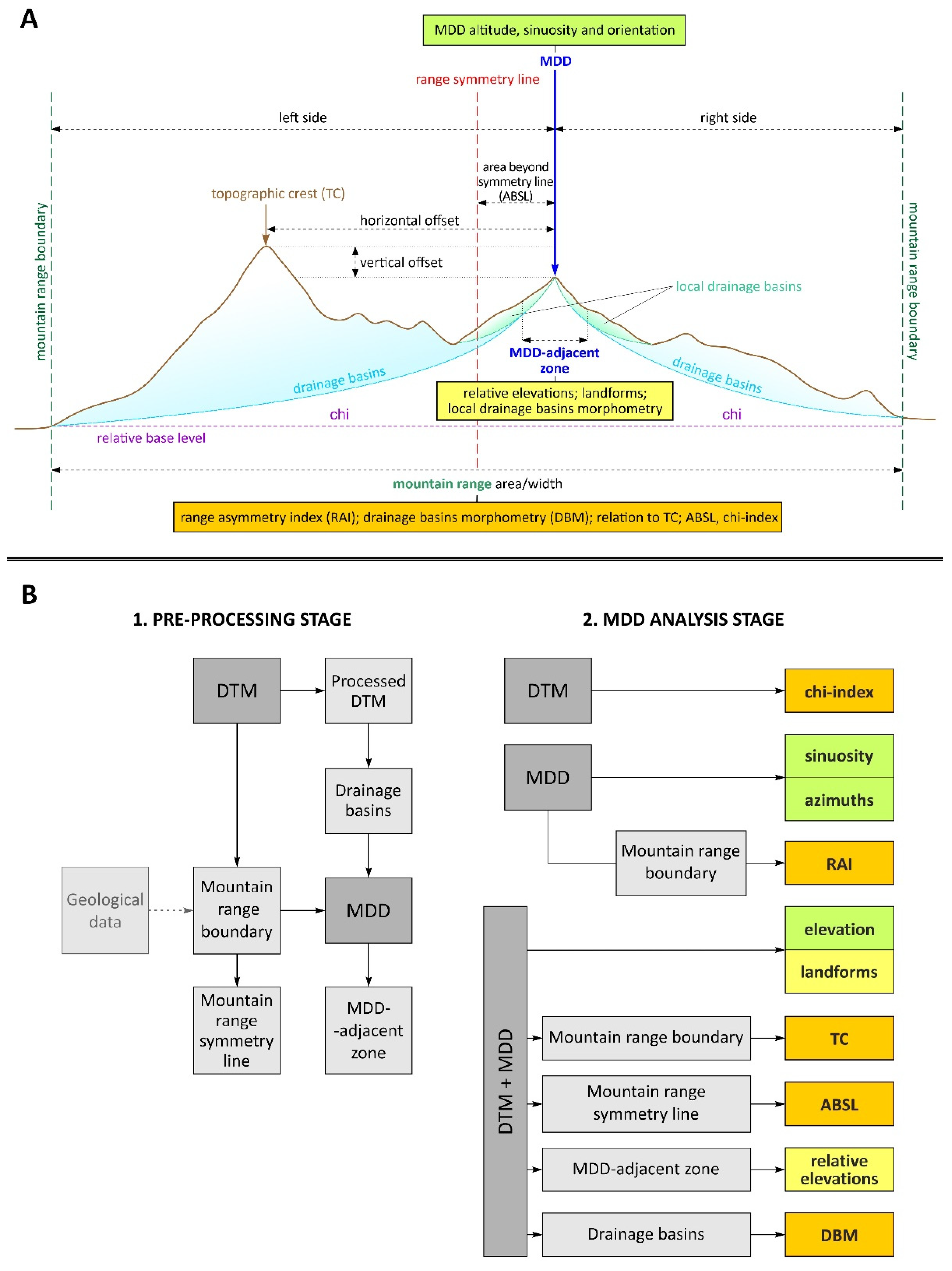
4. Measures to Characterize the Main Drainage Divide

The main section of the article is divided into three parts, reflecting the spatial dimension of each group of measures. The first group of measures (Section 4.1) focuses on the main drainage divide as a line running along the mountain range (1-dimensional). The relevant properties include the altitude change along the MDD, the sinuosity of the MDD, and the orientation of segments within the MDD (azimuth). The second one (Section 4.2) includes two-dimensional measures used to compare morphometric properties of two parts of the mountain range, located on the opposite sides of the MDD. The MDD is thus considered as a reference line to evaluate the symmetry/asymmetry of the range. The relevant measures are range asymmetry, morphometric properties of drainage basins on the opposite sides of the MDD, and the position of MDD versus maximum elevation within the range, also known as the Topographic Crest (TC). In the third group (Section 4.3) we also consider two-dimensional morphometric properties of the terrain, but the analysis is restricted to the close neighbourhood of the MDD, either forming a narrow belt parallel to it or bounded by the nearest distinctive topographic border (MDD-parallel major valley, fault-generated escarpments). This is based on an assumption that within a very wide mountain range of a complicated topographic structure, the relief characteristics of distal (peripheral) parts may have limited relevance to the MDD itself and its evolution immediately adjacent to the MDD, assuming that within a very wide mountain range of complicated topographic structure, relief characteristics of distal parts have limited relevance to the MDD itself and its evolution. These include parameters of drainage basins, topographic metrics related to relief energy and slope, longitudinal stream profiles, and synthetic relief representations derived from automatic landform classifications. Thus, more than ten properties in total are introduced and evaluated, but the list is certainly not exhaustive and further analytical tools may be added. Likewise, specific computational setups for particular properties may differ from those proposed by us, including the resolution change. Figure 2 shows schematically the spatial dimensions of these different properties of the MDD on an idealized cross-section of a mountain range and the flowchart followed in the analysis.

In the following sub-sections, each measure is presented using an identical template. The rationale behind its selection and information potential are presented first. This is followed by presentation of how a given measure was computed. The evaluation of the results of the exercise, carried out for the study area of the Sudetes, concludes each sub-section. These partial assessments are starting points to evaluate the whole ensemble, presented in Section 5.

4.1. Properties of MDD

4.1.1. Altitude

The altitude of the MDD and its change along a mountain range is a simple variable that can be directly derived from DEM and presented in the form of a longitudinal profile. Disregarding both geographical extremities of the range, where altitudes are expected to be low (unless the boundary is drawn at high-elevation cols, separating one range from another one), the MDD may run at a relatively constant altitude or show considerable up and down shifts, decreasing in altitude when crossing intramontane basins or low-lying passes. It may be hypothesized that the latter situation reveals either strong lithological or structural influence and, hence, the occurrence of more erodible zones within the mountain range, or the presence of down-faulted or otherwise depressed areas. However, descending altitudes of the MDD may also indicate geologically recent fluvial diversions (captures or overflows) or glacially conditioned rearrangements of valley networks (glacier transfluence sites). Thus, they potentially show places of drainage divide instability. Struth et al. [6] considered parts of the MDD profile that were below its average altitude as “drainage depressions” and suspected recent captures. Another feature of interest is the relationship between the altitude of MDD and the distribution of highest peaks within the range, which do not necessarily coincide (see Section 4.2.3).

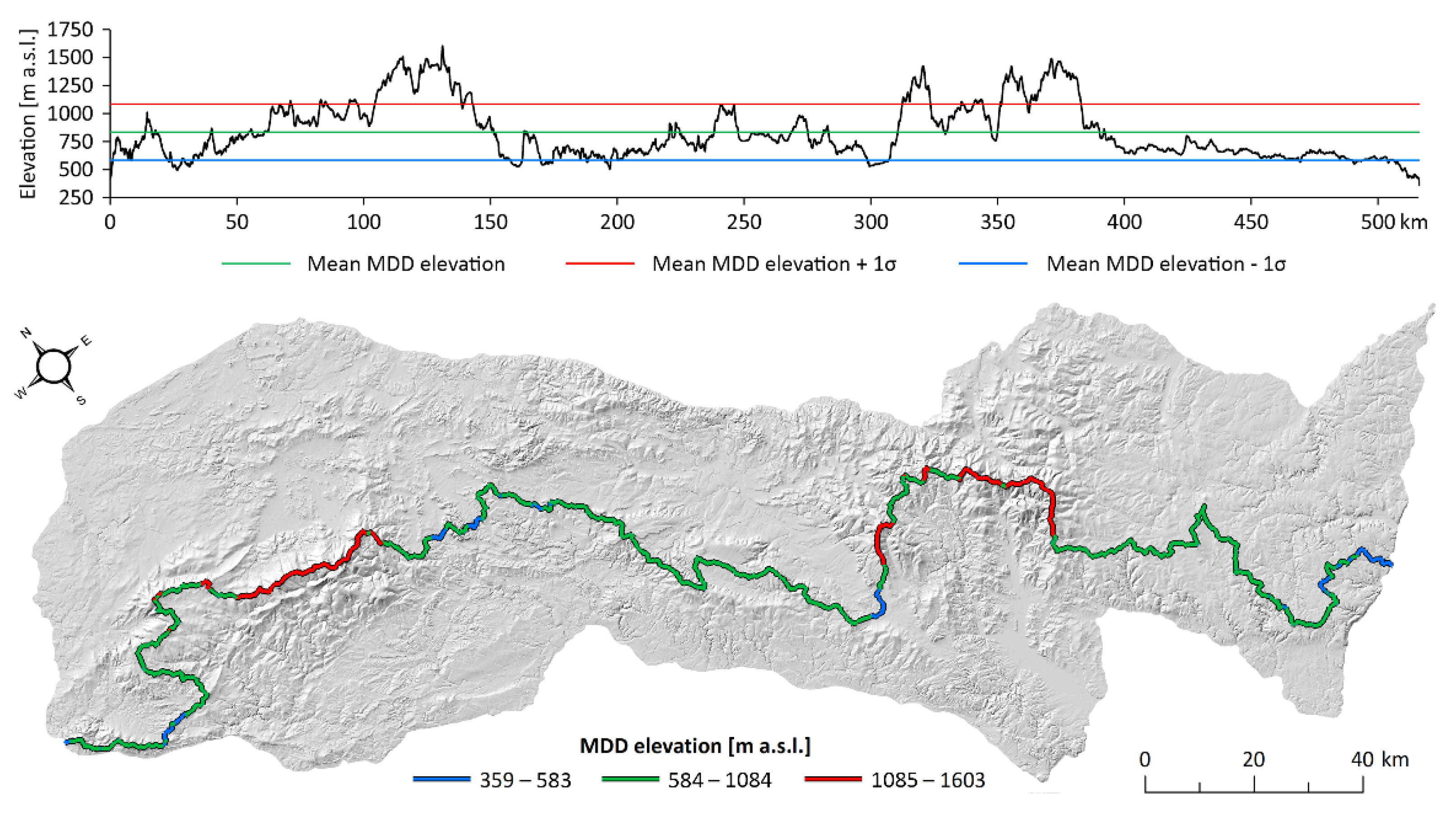
The elevation statistics of the MDD were calculated basing on DTM values located along the MDD line, in the constant interval of 20 m. Statistics included minimum, maximum, and mean values and the standard deviation. Consequently, the elevation values were reclassified in order to extract segments of particularly high and low elevations, using the criterion of mean + 1σ and mean − 1σ, respectively (Figure 3).

The MDD in the Sudetes covers an altitude range of 1244 m, with the mean value of 834 m a.s.l. and the lowest spot at 359 m a.s.l. at the SE extremity of the range, and includes the highest peak of the range (1603 m a.s.l.). Considerable jumps and drops in altitude are evident on the graph (Figure 2), but the analysis can be enhanced by applying simple statistical measures such as standard deviation. Consideration of altitudes above the mean + 1σ (>1085 m a.s.l. in our case) and below the mean − 1σ (<583 m a.s.l.) allowed us to recognize several notable topographic elevations and depressions along the MDD (Figure 3). However, the statistical distribution of altitudes along the MDD is important. In the Sudetes, the elevation of the MDD is right-skewed (skewness ~1). Therefore, MDD segments identified as excessively high are about twice as long as those excessively low (Figure 3). Nonetheless, a few notable depressions within the range were identified.

4.1.2. Sinuosity

Sinuosity is a measure that relates an actual length of a linear feature to the straight reference line, and its very use assumes certain meaning of the straight course, so that deviation from the straight line and its magnitude, expressed by the sinuosity index, has some information potential. In the context of drainage divides, a straight course indicates a similar pace of evolution of drainage basins on the opposite sides, where no gains or losses of catchment areas occur. By contrast, increasing sinuosity suggests more efficient, but localized headward erosion on one side, resulting in the enlargement of headwater parts of catchments and an upstream shift of the divide. The reasons for non-uniform erosion are multiple and may be related to the available relief, efficient spring sapping, the contributing role of landslides, or local lithological differences. Consequently, higher sinuosity might be expected at higher altitudes. At the mountain-range scale, the general interpretation of sinuosity is similar, and if the MDD follows a straight line, uniform erosion and evolution of drainage basins on both sides may be hypothesized. Drainage divide stability is likely to be associated with straight courses. However, at the large spatial scale, deviations from the straight line are caused by regional rather than local factors and may be related to non-uniform uplift; strong lithological control on erosional efficacy; considerable differences in climate conditions in different parts of a range (due to orographic barrier effect and decreasing maritime influences), particularly precipitation; or the length of time since the inception of the divide [4].

The sinuosity index (SI) is defined as:

$$SI=L/L_s$$

$L$—actual length of the divide; $L_s$—length of the straight line between end points.

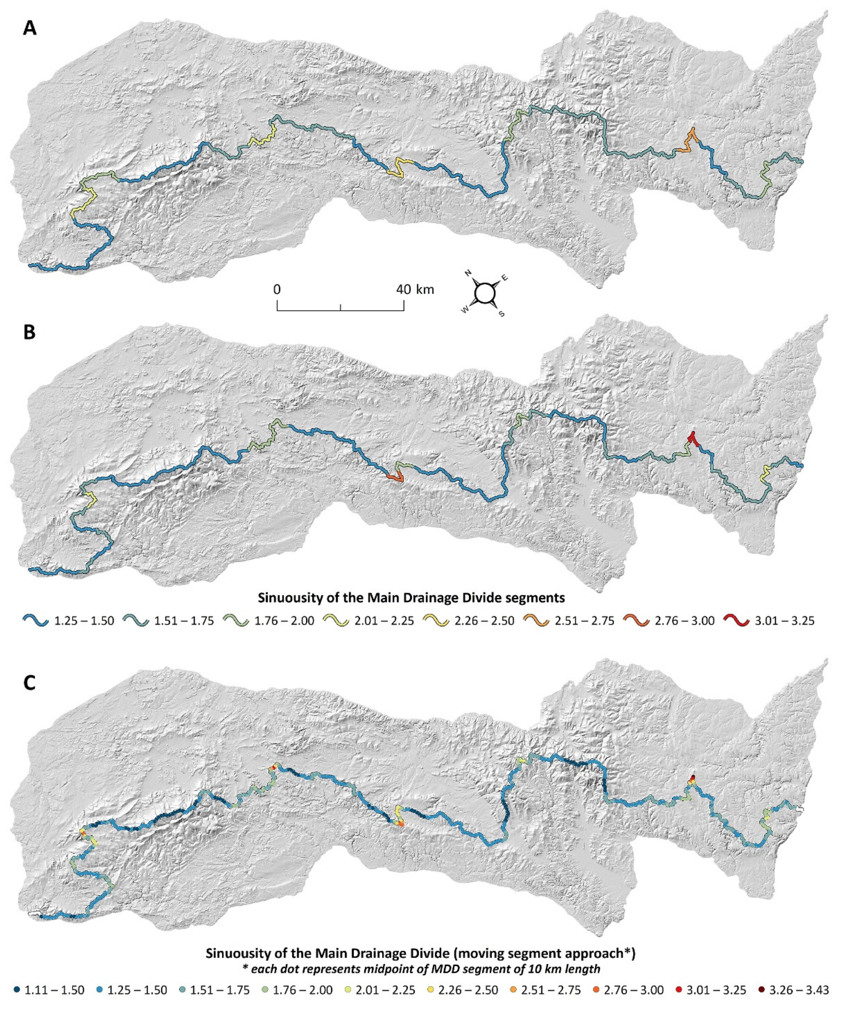
Its calculation is straightforward and involves the simple division of two values. More problematic is the decision regarding the end points, selected to derive the length of the reference straight line, and may involve an arbitrary determination of a point where the mountain range ends. Furthermore, a single (mean) value for the entire range will only be useful if it can be compared with similar values derived from other ranges. However, the variability of SI within a mountain range may have significant information potential but requires slicing the MDD into shorter segments according to a predefined value. In our exercise, two divisions were used, into 10 and 20 km long reaches, so that SI was calculated for more than 50 and 25 sections, respectively. These were considered most meaningful for the ~500 km long MDD of the Sudetes, but in other areas different lengths may be more useful. Realizing the rather arbitrary choice of slicing, we also used a moving-segment approach, setting its length for 10 km and a movement distance of segment endpoints along the MDD line for 1 km. In addition, we calculated SI for 100 m height intervals to check if there is any preferential association between altitude and sinuosity, which might suggest elevation-dependent different pathways of MDD evolution, assuming that higher sinuosity indicates less uniform headward erosion.

The SI value for the entire MDD of the Sudetes was 2.1. The spatial pictures of SI variability for 10 km and 20 km long sections are fairly similar (Figure 4), typically below 1.75 (more than 70% of the total length), but there a few notable exceptions, with much higher values, up to 3.25. They are all related to deep indentations of the MDD rather than to significant small-scale variability, as confirmed by the picture for 20 km slicing. The use of a moving segment (Figure 4C) yielded similar results, identifying the same sectors of the MDD as the most sinuous but also emphasizing short sectors of extremely high or low sinuosity. Examination of the relationship with altitude did not reveal any specific pattern, with all average values for 100 m height intervals within the 1.0–1.5 range of SI.

4.1.3. Orientation

Orientation complements the sinuosity index and informs about the preferential direction(s) followed by the MDD, which may, or may not, coincide with the general strike of a mountain range. Significant coincidence may indicate a relatively simple history of geomorphic evolution of the range, with rather uniform development of drainage basins on its opposite sides. However, this is not equal to the persistence (stability) of the divide, because uniform migration in one direction, perpendicular to the range extension, will produce a similar effect. By contrast, considerable diversity of directions likely suggests complex geomorphic development, reflecting either non-uniform headward erosion on the opposite sides of the divide or the presence of multiple second-order morphostructures within the boundaries of the range, with their own uplift/subsidence histories. An over-representation of directions perpendicular to the strike of the range may point to the existence and significance of transversal structures, which focus erosion and hence, indirectly, contribute to the emergence of MDD sections inconsistent with the general direction.

Quantitative analysis of MDD orientation was based on segments of constant length of 100 m. Each segment was transformed into a straight section connecting both endpoints, allowing one to calculate the line bearing and assign it into one of eight orientation classes: N–S, NNE–SSW, NE–SW, ENE–WSW, E–W, ESE–WNW, SE–NE, and SSE–NNW). A further procedure included the calculation of percentages of each orientation class in the total MDD length, as well as in segments located within selected morphostructural units. The illustrative plots were generated using the Polar Plots ArcGIS extension [28].

In the Sudetes, shares of different directions vary within the 9–17% range of the total—hence, nearly by the factor of two (Figure 5). The highest representation typifies the SE–NW direction, coincident with the general strike of the range, but, taken alone, it accounts for less than one fifth of the total length of the MDD. Even if combined with two adjacent directions (ESE–WNW and SSE–NNW), it is still less than half of the total length. Among the remaining directions, N–S and E–W are most represented. Altogether, this distribution pattern suggests a complicated history of drainage organization within the range, although taken alone it does not reveal the underlying reasons.

Analysis of the orientation of the MDD can be extended, with exploration of various spatial relationships. For example, sub-regions within a range may be analysed separately in order to identify areas with different MDD orientation patterns. Figure 5 illustrates that the dominant directions of the MDD may be considerably different between individual minor geomorphic units within complex relief. In the Sudetes, sector 1 shows the very consistent dominance of the NW–SE direction, which is also present in sector 3; so, these two broadly follow the extension of the entire range. In sector 2, the pattern reveals the preference for the W–E to the NW–SE directions. However, the East Sudetes show a different pattern, with a significant contribution of the NE–SW direction (sector 4) and the NNE–SSW (sector 5), hence perpendicular to the range.

4.2. MDD as a Reference Line for Range Symmetry

4.2.1. Range Asymmetry

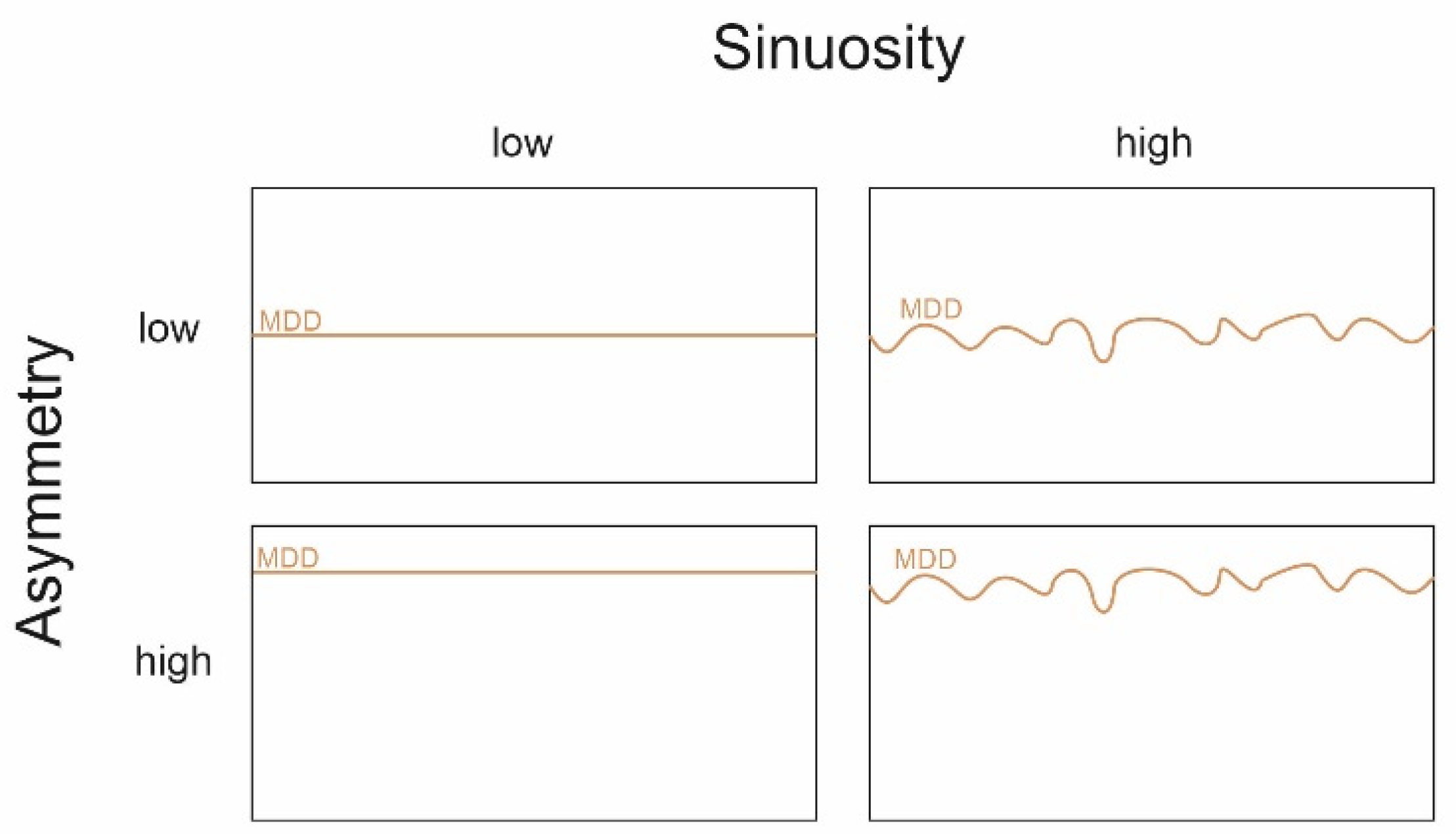
Except for rare cases of ubiquitous transversal drainage, mountain ranges separate areas drained in opposite directions, with the main drainage divide acting as a boundary. The MDD may run more or less along the central part of the range, or it may be shifted towards one of its topographic boundaries. If the latter occurs, the range becomes asymmetrical in the sense that the two parts located on the opposite sides of the MDD are of unequal size. This may correspond to non-uniform distribution of other variables such as average slope, with the smaller area being steeper. A lateral shift of the MDD may be consistent along the range, or it may alternate from one side to the other, accounting also for considerable sinuosity of the MDD at the range-scale. However, these two properties convey different messages, as illustrated by Figure 6.

Asymmetry in location of the MDD within the range is addressed by the Range Asymmetry Index (RAI), which expresses this property quantitatively and may be calculated for both the entire range and swaths of predefined width, perpendicular to the strike of the range, following the formula:

$$\mathrm{RAI}=\left|\frac{{\mathrm{A}}_{\mathrm{L}}-{\mathrm{A}}_{\mathrm{R}}}{{\mathrm{A}}_{\mathrm{L}}+{\mathrm{A}}_{\mathrm{R}}}\right|$$

where ${\mathrm{A}}_{\mathrm{L}}$ and ${\mathrm{A}}_{\mathrm{R}}$ are the areas of the mountain range on the opposite sides of the MDD. In our case, the NE side of MDD was considered “left.” Ideal symmetry will result in the RAI value of 0, whereas the value close to 1 would indicate extreme asymmetry.

In the Sudetes, the main watershed divides the range into two unequal parts, with the RAI equal to 0.2 and the NE side occupying c. 60 per cent of the area (Figure 7). However, this range-long asymmetry does not result from a consistent shift in the MDD to the south-west, as demonstrated by the jagged course of the separating line on Figure 7A and the variability of the RAI (Figure 7B). Along the entire range it is only the central-western part (from 45 to 83 km and 90 to 110 km) where the MDD runs relatively close to the theoretical line of equal division (RAI < 0.2). In the rest of the area one can identify several considerable shifts of the MDD to SW, so that the SW side accounts for less than 40% of the range width. By contrast, only one evident shift to NE occurs, between 155 and 185 km, but it is very prominent. Locally, the percentage of the SW-drained side of the range exceeds 80%, resulting in the RAI exceeding 0.6.

4.2.2. Properties of Drainage Basins on the Opposite Sides of MDD (Range-Scale)

Further insights into the asymmetry of a range can be obtained from a comparative analysis of morphometric properties of drainage basins located on the opposite sides of the MDD. In this exercise, basin outlets are located at the topographic boundaries of the range, and the basins are considered in their entire extent. At the same time, only basins bordered by the MDD are taken into account. This setup allows one to expect similarities within each side of the range, as well as between the two sides, for symmetrical ranges, whereas asymmetric ranges will likely show dissimilar morphometric properties of drainage basins on the opposite sides. In the specific case of multiple lateral shifts of the MDD along the range, high variability is also expected within each side.

The selection of morphometric variables is decided by the operator, but in general it may include various measures applied to drainage basin characteristics [29,30,31], especially those used in morphotectonic studies. In this study, variables related to both relief (hypsometric integral, mean slope, percentage of slope above 20° within the entire basin, and within the 500 m buffer zone from the MDD) and basin shape (compactness and circularity) were used to characterize 41 drainage basins (

Table 1. Morphometric differences between river basins on the opposite sides of the MDD in the light of statistical tests. Asterisks indicate p-values significant at ¦Á = 0.05 (*) and a = 0.01 (**).

Parameter	Range-Scale (See Figure 7A)	Incised into the MDD (See Figure 7B)	Within Second-Order Morphostructures (See Figure 7B)
			I	II	III	IV	V
Hypsometric integral	0.029 *	0.566	0.713	0.255	0.036 *	0.346	0.013 *
Mean slope	0.052	0.207	0.046 *	0.366	0.148	0.818	0.002 **
$\mathrm{Slopes}>20°$ (%)	0.139	0.333	0.220	0.360	0.355	0.496	0.024 *
$\mathrm{Slopes}>20°$ within buffer zones (%)	0.999	0.708	0.986	0.222	0.791	0.555	0.856
Basin compactness	0.003 **	0.041 *	0.894	0.002 **	0.006 **	0.295	0.319
Basin circularity	0.013 *	0.000 **	0.102	0.060	0.000 **	0.718	0.329

; Figure 8A). To examine morphometric differences between river basins on the opposite sites of MDD, statistical testing was carried out. The probability distribution of residual values of morphometric variables, which determines whether a parametric t-test (if the distribution is normal) or its non-parametric alternative (Mann–Whitney–Wilcoxon test) should be applied, was assessed by a Shapiro–Wilk test for normality. The homogeneity of variance, important in terms of the application of Welch’s correction in the parametric test, was examined by Levene’s test.

In terms of relief, the SW side of the range proved steeper (supplementary Material), but the differences within the range of 1.5–3.75° are not significant statistically. By contrast, the value of hypsometric integral is markedly higher for the SW side and is statistically significant. Two variables relevant to the shape of basins have values that are significantly different for the opposite sides of the range, with higher values typifying the SW side. These values are interpreted to characterize areas subject to less uplift and more advanced denudation, which are the conditions allowing for more efficient drainage integration and lateral growth of drainage basins [31,32]. Even though the rationale for such an explanation is not entirely clear, it is nevertheless significant that the two groups of indicators did not provide an unequivocal picture and consistent information, making interpretation difficult. However, two factors may have influenced the results of the exercise. First, in response to lateral shifts in the MDD, the areas and number of basins vary considerably, so that basic observation units may not be fully comparable (Figure 8A). Second, and perhaps more importantly, the complex topography of the Sudetes results in considerable relief heterogeneity of the basins, especially on the NE side. They include both fairly steep relief close to the MDD and much more subdued topography far away from the MDD, yielding average values of uncertain meaning. Therefore, a similar exercise was also carried out for much smaller drainage basins within individual blocks (morphostructures) inside the Sudetes, crossed by the MDD (see Section 4.3.4).

4.2.3. MDD Versus Topographic Crest and Synthetic Divide

The main drainage divide may connect the highest peaks of the range, but it is also possible that these are located beyond the MDD, within second- and higher-order divides radiating from it, within parallel ridges disconnected from the MDD, or as isolated elevations away from the MDD. For example, Forte et al. [11] have shown that this is the case in the Greater Caucasus and the line connecting the most elevated peaks (“topographic crest”), identified within range-perpendicular swaths of predefined width, is not coincident with the MDD, running consistently to the north of it. This offset was interpreted in terms of regional tectonic history as the evidence of northward propagation of deformation and the younger age of the topographic crest in relation to the drainage divide [33]. Another approach to examine spatial coincidences or inconsistencies at the subcontinental scale involves delimitation of a “synthetic drainage divide” [34,35]. It is an outcome of filtering of topography at short (50 km), medium (100 km), and long (150 km) wavelengths, which eliminates topographic features with spectral dimensions below the given wavelength. The “synthetic drainage divide” is believed to reflect the operation of various endogenic processes that produce crustal deformation due to both crustal tectonics and dynamic mantle influences. The method leads to the identification of areas where the positions of the actual and “synthetic” divide differ, opening the room for various explanations. Furthermore, these spatial offsets can be quantified using the root-mean-square deviation, and the wavelength-dependent best fit of a filtered topography to the actual drainage divide can be calculated. This approach has been used to such contrasting geodynamic settings as the northern Rocky Mountains [34], the Rif Range and Betic Cordillera, and the Appalachians [35], leading to the general conclusion that the position of the divide is largely controlled by exogenic processes, which may modify to variable extent long-wavelength topography arising from crustal processes.

The idea of a topographic crest may work properly in mountain ranges with well-defined axial ridges but is more difficult to implement in horst-and-graben relief such as represented by the Sudetes. Indeed, the highest spots within swaths alternate between two sides of the MDD, and, in consequence, a continuous topographic crest would not be a very meaningful feature along the entire range (although it can be identified within specific areas). Therefore, a different approach was tested. The range was divided into 100 m wide swaths perpendicular to the sides of a rectangle that encompasses the entire range using the minimum bounding geometry principle (Figure 9A). Within each swath, the position of the MDD and the location of the highest spot were indicated. The latter may lie on the MDD, but this is not necessarily the case (Figure 9A). This approach also helps to visualize altitude variability within each swath, highlighting the relative elevation of the MDD (compare the upland part in the east versus a relatively narrow, but most elevated ridge in the west, between 40–65 km). Graph B compares the altitude variability along the MDD with altitudes of the highest spots within each swath along the range, both in terms of absolute height (top) and height difference (bottom). Finally, graph C informs about the horizontal offset between the MDD and the maximum altitude, including the direction. To complete the information, selected cross-sections illustrate different spatial and altitudinal relationships between the MDD and the highest spots within specific parts of the range (Figure 9D).

This approach revealed the considerable complexity of topographic and altitude relationships within the range. There are only a few sections of the MDD, where it coincides with the highest elevations. For example, 200–300 m large vertical offsets in the central part of the Sudetes, at 85–135 km, are associated with the presence of prominent second-order mountain crests, which are not followed by the MDD. These may be completely disconnected from the MDD (Sowie Mts., Kamienne Mts.), or run parallel to the MDD, in close distance (Orlické Mts.). Physical separation of the MDD and the line of highest altitudes (horizontal offset) vary considerably too, reaching as much as >30 km (note that the mean width of the range was 59.2 km) (Figure 9C). Characteristic are isolated spikes, indicating horizontal offset by >10 km (up to 30 km in extreme case). These are related to localized high elevations quite far away from the MDD. Explanations for these offsets are of different kinds and include higher rock resistance, resulting in isolated peaks and massifs (Kamienne Mts.), as well as the presence of second-order uplifted areas within the range-scale block-faulted topography (Sowie Mts.).

4.3. Morphometric Characteristics of Terrain Adjacent to MDD

4.3.1. Properties of Areas beyond the Theoretical Symmetry Line

Overlying the actual course of the MDD and the position of the range symmetry line (RSL) will reveal areas located far beyond this line but drained towards the opposite side of the range. Since the shifts in the MDD themselves may carry information about the history of drainage pattern development, it is reasonable to assume that such areas may have specific geomorphometric signatures too. For example, if the shifts are due to aggressive headward erosion from one side, a higher total relief and a higher mean slope but a lower mean elevation may be expected for these areas. Consequently, morphometric parameters similar to those applied to drainage basins can be used to characterize such terrains. This exercise, if coupled with examination of other measures such as cross-divide differences in chi-values (see Section 4.3.2) may aid interpretation whether such indentations of the MDD are actively expanding by headward erosion and likely to gain areas or are rather remnant surfaces surrounded by aggressively eroding streams and destined for area loss.

In the first step, the symmetry line of the range (RSL) was drawn, and this was done by two alternative methods. Approach 1 involved drawing a minimum bounding rectangle over the mountain range area (delimited in respect to topography, see Section 3), which was then divided into two minor rectangles of equal size by the RSL (Figure 10A). In the second approach, the RSL was derived as the line of equal Euclidean distance from NE and SW boundaries of the mountain range. In contrast to approach 1, the resultant RSL is not a straight line, but it mirrors the actual boundaries of the range (Figure 10B) and, therefore, is more suitable for mountain ranges, which are arcuate. It was further assumed that a certain degree of sinuosity of the MDD is its inherent feature, and, hence, it is the area located well away from RSL that should focus most attention as anomalous positions. To account for this, an envelope with the width of 1 σ of the distance between RSL and the MDD was drawn along the symmetry line, and morphometric properties were calculated for areas beyond this envelope. Figure 10 shows that in each approach the location and proportions of areas beyond RSL are different.

Variables taken into account included the hypsometric integral, the mean slope, the percentage of low relief (<5°) and steep terrain (>20°), and two measures related to planform (

Table 2. Morphometric properties of areas located far beyond the symmetry line of the Sudetes range and drained towards the opposite side of the range (see Figure 9 for location).

ID	Area (km2)	Hypsometric Integral	$\mathbf{Mean}\mathbf{Slope}(°)$	Percentage of Areas		Sinuosity	Shape Ratio
				$<5°$	$>20°$
Approach no. 1 (see Figure 9A)
1	618.9	0.291	8.9	36.4	8.7	5.90	0.84
2	3.8	0.498	7.4	23.8	0.3	1.53	9.00
3	1.7	0.388	11.3	22.1	15.3	2.45	1.58
4	48.3	0.291	7.8	35.7	4.3	2.38	2.37
5	64.0	0.434	16.1	6.9	30.4	2.00	5.94
6	50.1	0.544	4.9	68.1	1.9	2.75	2.08
Approach no. 2 (see Figure 9B)
1	468.8	0.289	9.4	31.8	9.4	4.47	1.01
2	12.0	0.478	13.2	8.3	14.2	1.27	6.07
3	11.0	0.482	13.9	7.7	18.3	2.03	3.23
4	65.9	0.270	8.4	34.0	5.6	1.81	2.92
5	131.2	0.358	13.4	10.1	17.3	1.80	1.83
6	138.9	0.256	6.4	45.7	1.3	1.69	2.74
7	108.9	0.551	5.4	61.6	2.4	2.61	1.97

). These were labelled the “sinuosity” and the “shape ratio.” The former indicates how contorted is the section of the MDD within an area beyond the symmetry line and is a simple proportion of the length of MDD to the length of RSL within each such area. High values show multiple projections of the MDD away from the RSL, suggesting active headward erosion. The latter is obtained through dividing the maximum width of the area beyond the symmetry line by its depth, measured in the perpendicular direction to the width. Low values of this ratio show prominent finger-like extensions beyond RSL, whereas high values denote a limited lateral shift of the MDD.

A small number of areas beyond the symmetry line in each approach precludes statistical data treatment and testing for significance of differences. In addition, some of these areas are extremely small. Therefore, only a qualitative description can be provided, based on summary results in Table 2. The areas analysed vary in terms of each measure considered, showing a range of values, from low to high. For example, in terms of the mean slope they vary within the range of 4.9–16.1° (approach 1) and 5.4–13.9° (approach 2). Differences in terms of percentage of low-angle versus steep slopes are even more evident. In approach 1, the area no. 5 emerges as particularly steep, whereas the area no. 6 shows very subdued relief at relatively high altitude, as indicated by the highest value of HI. In approach 2, these two areas are broadly equivalent to areas no. 5 and 7, respectively, showing comparable characteristics. Among two planform measures, the sinuosity ratio is consistently very high at the westernmost part of the range (area no. 1 in each approach). The shape ratio shows relatively low values for large areas no. 5 and 7 in approach 2, indicating considerable distance from RSL. Thus, both these areas appear anomalous in the light of several, rather than just one, variables.

4.3.2. Longitudinal Stream Profiles (Chi-Index)

Analysis of longitudinal stream profiles by means of the chi(χ)-index [15] is perhaps the most common method to approximate the intensity of ongoing erosion on the opposite sides of a drainage divide. Derivation of the chi-index and possible visualizations have been described in numerous publications, and the reader is referred to these sources [16,17,18,36]. In the context of drainage divide (in)stability, it is generally assumed that lower values of chi indicate more vigorous long-term erosion and an upstream shift in the stream source. Hence, contrasts in chi-values on the opposite sides of a divide are interpreted in terms of divide migration and used to predict localities of future captures [6,16,17,18,37]. However, this approach works best if uplift pattern, bedrock erodibility, and climatic conditions are uniform, which is hardly the case for long mountain ranges and prominent orographic barriers [10,38]. Having said that, across-divide differences in chi-values remain a useful tool to analyse geomorphic properties of the MDD and to assess its possible segmentation, especially if anomalies (discrepancies) can be evaluated against information about lithology and structure and checked against other topographic metrics for the same localities.

The chi-index was calculated using the LSDTopoTools software package (version 2) designed to analyse topography [39,40]. For channel extraction, the channel extraction tool was applied [41]. For calculation of chi, the Chi Mapping Tool was used [35]. The following parameters were used to select channels and basins: (a) the threshold contributing area to initiate the channel—3000 raster cells; (b) the minimum basin size—3000 cells; and (c) the maximum basin size—40,000,000 cells. For the chi-index mapping, we used the concavity of the channel profile parameter m/n = 0.4, which was confirmed to be optimal for most of the basins in the study area. To compare chi-values across drainage divides [16], it is recommended to set outlets at the same elevation. For the Sudetes, we adopted a base level of 300 m a.s.l. 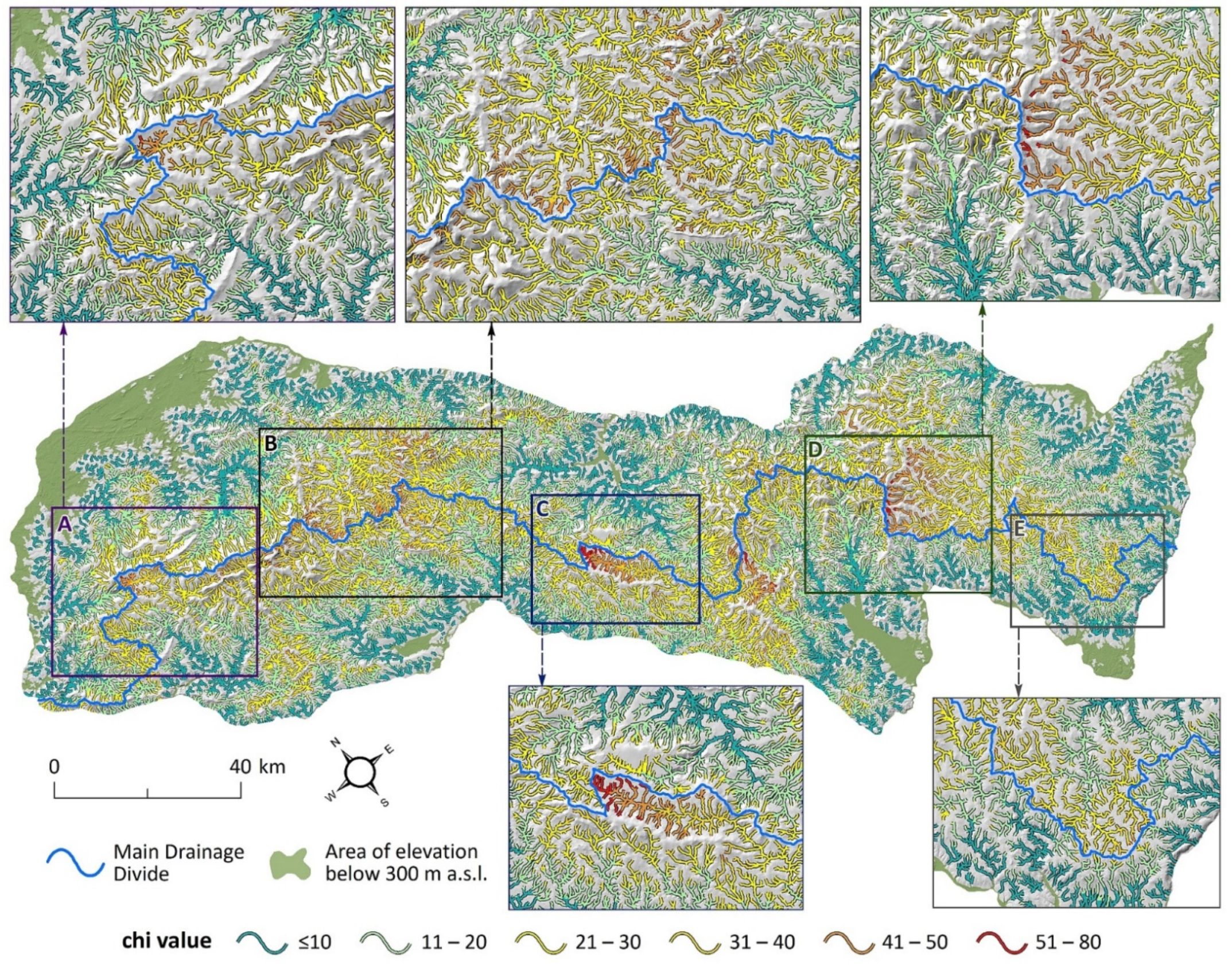that allowed us to include most of the range in the analysis, except a few low-lying peripheral areas, especially in the north-west (Figure 11). The resultant map was then clipped to the area of the Sudetes.

Examination of chi-values along the MDD reveals a complex picture, with sections representing dissimilar spatial patterns alternating along the length of the Sudetes (Figure 10). Three variants occurred. Variant 1 indicates no evident differences between the opposite sides of the MDD; variant 2 shows higher chi-values to the south-west of the MDD; whereas variant 3 represents a reverse situation, that is, the presence of higher chi-values to the north-east of the MDD. The latter contrast dominates along the MDD and appears in the central part of the range (area B) but is most striking in its eastern sector (areas D and E). In each of these cases, there is no clear lithological difference between the opposite sides of the MDD that could account for this asymmetry. Likewise, each of these areas represents specific geological setting, unlike the others (Figure 1B). By contrast, variant 2 is much less represented and appears most clearly in the central part of the Sudetes, where high chi-values are associated with an intramontane graben of the NNW–SSE strike (area C). Moderate differences are also recognized in the highest part of the Sudetes (area A) and suggest more vigorous erosion in drainage basins located to the north of the MDD. Variant 1 occurs locally, mainly in the central-east part of the Sudetes. Overall, if the most common interpretation of chi-values is followed, one can argue for different long-term trends in MDD stability and hypothesise future migration of the MDD to the north in the eastern part of the Sudetes and locally in the central part, but the southward shifts in many places in the western part of the range. This will result in a further increase in sinuosity of the MDD.

4.3.3. Topographic Asymmetry

In addition to topographic metrics suggested by Scherler and Schwanghart [7,8] and Forte and Whipple [10] to be useful indicators of potential drainage divide instability, we propose another complementary measure that allows to capture the asymmetry of the relief along the MDD (crest shape), without relating it to the nearest stream and the depth of incision. Thus, it can be applied in mountains lacking well-developed drainage systems in the neighbourhood of the main divide (e.g., in karst). The quantitative parameterization of areas adjacent to the MDD was based on the zonal elevation range (local relief) approach. The MDD was divided into 5 km long segments, and each segment had its adjacent zones (“left” and “right”) assigned with the use of the Euclidean Allocation ArcGIS tool. The spatial extent of such zones was limited by the buffer of 1 km from the MDD line on either side, which in our study area captured across-divide differences in steepness sufficiently well and may be considered a lower spatial limit of meso-relief [42]. The MDD segment length was chosen deliberately in order to minimize differences between surface areas of paired left/right zones. This problem was caused by local sharp turns in the MDD, and the magnitude of differences grows proportionally to the shortening of the length of MDD segments. In the next step, the elevation range (ΔH = H_max − H_min) was calculated for each zone, followed by an assignment of ΔH_left and ΔH_right values to each MDD segment. In consequence, it was possible to calculate the ΔH difference (ΔH_diff = ΔH_{left −} ΔH_right) and, finally, absolute ΔH_diff values. High values of ΔH_diff indicate segments distinguished by topographic asymmetry of adjacent areas located on the opposite sides of the MDD.

The following characteristics of the MDD belt emerge from this exercise. Relief asymmetry along the MDD varies in the Sudetes (Figure 12), from less than 25 m to more than 150 m (with the maximum value of nearly 190 m), with frequent alternations between high and low values along the length of the divide. Taking the range in its entirety, the NE side is steeper along 55% of the length of the MDD, but it is generally steeper in the western part of the Sudetes, whereas in the eastern part of the range it is the SW side that almost consistently has more relief. Of interest are some short-wavelength major across-divide shifts of higher relief, such as at 320–330 km and 370–380 km, apparently indicative of competing strong headward erosion on the opposite sides of the MDD.

4.3.4. Properties of Drainage Basins Incised into the Dividing Ridge

Here, the computational approach is identical to the one presented in Section 4.2.2, but the reference drainage basins are different. Morphometric properties are calculated for basins, which are still limited by the MDD on their upstream sides, but their lower boundaries (basin outlets) are located at the nearest junction of mountainous terrain with lower ground, be it an intramontane graben, basin, wide trunk valley, plain, or mountain foreland. This alternative approach is based on an assumption that processes involved in the evolution of the MDD are mainly related to the topography of its nearest vicinity rather than to the characteristics of distant parts of the range, included in the computation of morphometric properties at the range scale (see Section 4.2.2). This approach may be more meaningful for mountain ranges of highly complex morphology, where large-scale relief may be additionally resolved into a mosaic of second-order structures at higher and lower elevations. These structures can be related to non-uniform uplift, rock-controlled differential erosion, or other causes. Additional possible advantages of this approach include a larger number of observation units and a narrower range of the drainage basin area variable, both allowing for more informed statistical treatment. However, the use of this setup necessitates the presence of inner escarpments/mountain fronts and will hardly work if the MDD runs within an intramontane basin.

The first step in this part of the procedure involved delimitation of specific areas, for which the exercise would be meaningful. Five such areas, considered as separate morphostructures with clearly outlined topographic boundaries, were distinguished (Figure 8B), representing narrow ridges (I), large and considerably elevated blocks (II, III, and IV), and uplands (V). The number of drainage basins within each area is as follows (N/NE side versus S/SW side): I—11/12, II—27/6, III—26/10, IV—12/11, and V—9/9. The subsequent procedure was identical as described in Section 4.2.2., including the choice of variables. In the final phase, tests for statistical significance of differences were carried out for both the entire range and for each of the five morphostructures separately. In the latter approach, the morphostructure (II) was also included despite a low number of drainage basins on the S side, so that results of statistical testing in this case have to be treated with caution.

Taking the entire length of MDD into account, the results did not reveal any evident differences between the opposite sides of the divide in terms of steepness. Mean slopes differ by less than 1°, and the percentage of steep slopes (>20°) is only marginally higher on the NE side (by 2.5%). Thus, the NE side appears steeper (contrary to the situation presented in Section 4.2.2.) but not to the extent of statistical significance. By contrast, the values of shape measures are statistically different, but the higher values are now ascribed to the NE side. Thus, the approaches described in Section 4.2.2 and Section 4.3.4 yielded different results, and it seems that populations of drainage basins on the opposite sides of the MDD do not have distinctive morphometric signatures each. Considering the five morphostructures separately, the following observations emerge. In neither case are all parameters computed for each side statistically different from their counterparts on the opposite side (Table 1). The higher number of differences applies to blocks III and V (three for each morphostructure), although in block III they typify basin shapes, whereas in block V the steepness of the terrain is different. In each case the values of HI are statistically different. Differences in the mean slope and the percentage of slopes above 20° (both within the basins and inside the buffer zone) seem quite clear for several morphostructures (e.g., steep slopes in blocks I and III and steep slopes in the buffer zone in block II and III), indicating that the N/NE side is steeper, but they proved not to be statistically significant. Actually, if only the 500 m buffer zone is considered, in none of the seven cases examined the opposite sides of the MDD proved different from the statistical point of view (Table 1).

4.3.5. Relationship to Large-Scale Relief

Mountain ranges are not necessarily homogeneous in terms of internal relief, and beside prominent ridges, they may also include high-elevation plains, broad terrain convexities, and intramontane basins and corridors. Long-term behaviour of a drainage divide in each such type of relief may be different, in terms of both its previous history and future stability. Hence, it might be useful to know spatial relationships between the MDD and relief at a larger scale. For example, a significant part of MDD within planar relief at high elevations may suggest recent plateau uplift and delayed headward erosion, whereas the coincidence of the MDD with low-lying surfaces (valleys) may result from recent downfaulting. Theoretically, objective insights into these relationships can be obtained from the examination of results of automatic relief classification.

In this study, three automatic classifications were used. Two of them were based on the Topographic Position Index (TPI) [43], whereas the third one used the concept of geomorphons [44]. The former is calculated as the difference between the altitude in a given location and the average altitude in a pre-defined neighborhood [45]. On this basis, two classification systems were developed: (a) Slope Position Classification, which allows to distinguish six basic landforms, and (b) Landform Classification, using a combination of TPI calculated for small and large neighborhood, which allows one to distinguish ten nested landforms [43]. The latter is based on the concept of geomorphons, considered as elementary terrain units. Theoretically, it is possible to distinguish 498 geomorphons, independent of the relief, the size, and the orientation, possible to generalize into ten basic landforms [44]. The results for both classifications are strongly dependent on the adopted parameters such as the size and shape of the neighbourhood in TPI-based classifications and search radius and relief (angle) threshold in geomorphon-based classification. The parameters should be adapted to characteristic relief features in the analysed area, but in areas with heterogeneous relief, such as the Sudetes, their arbitrary determination is not an easy task. In this analysis, two values of the search radius were used (100 and 500 m), and five possible threshold angles were tested, from 1 to 5 degrees. Simplifying landform classes in both classifications, one can assume that rugged, mountainous terrain is represented by the association of ridges, upper slopes, and midslopes in the TPI approach, whereas in the geomorphon approach, the respective combination is ridge, shoulder, spur, and slope. By contrast, low relief consists of valleys, toe slopes, and plains in the former and flat, footslopes, valleys, and depressions in the latter.

The results proved interesting for two reasons. First, they confirm that in the Sudetes the MDD runs across different types of relief and sharply outlined ridges are but one possible topographic expression of the MDD (

Table 3. Results of TPI- and geomorphon-based landform classification along the MDD using various computational settings (RL—radial limit; TA—threshold angle). All values are percentages.

TPI-based	Landform			Valleys	Toe slopes	Plains	Midslopes	Upper slopes	Ridges
	Computational setting	RL = 100 m		1.1	1.3	20.8	3.6	18.5	54.7
		RL = 500 m		4.8	0.5	1.2	0.3	0.9	92.3
		Small scale = 100 m Large scale = 500 m		Canyons, deeply incised streams	Midslope drainages, shallow valleys	Upland drainages, headwaters	U-shaped Valleys	Plains	Open slopes	Upper slopes, mesas	Local ridges, hills in valleys	Midslope ridges, small hills in plains	Mountain tops, high ridges
				0.0	0.2	0.0	0.2	36.2	6.1	29.3	0.0	1.6	26.4
Geomorphon-based	Landform			Flat	Summit	Ridge	Shoulder	Spur	Slope	Hollow	Footslope	Valley	Depression
	Computational setting	RL = 100 m	(TA = 1)	2.9	3.4	30.9	6.0	28.7	27.2	0.2	0.6	0.1	0.0
			(TA = 2)	12.9	1.9	23.8	10.9	23.6	25.7	0.1	1.0	0.1	0.0
			(TA = 3)	24.4	1.2	18.8	12.2	19.4	22.8	0.1	0.9	0.0	0.0
			(TA = 4)	33.7	0.8	15.6	13.0	15.7	20.2	0.1	0.9	0.0	0.0
			(TA = 5)	41.6	0.5	12.8	13.7	12.6	17.6	0.1	1.0	0.0	0.0
		RL = 500 m	(TA = 1)	0.4	11.1	51.6	4.0	22.0	10.4	0.4	0.1	0.1	0.0
			(TA = 2)	5.2	7.0	45.8	12.6	17.9	10.8	0.1	0.6	0.1	0.0
			(TA = 3)	14.6	4.4	39.9	16.0	14.5	9.5	0.1	0.9	0.0	0.0
			(TA = 4)	24.4	2.9	34.7	16.7	11.9	8.4	0.1	0.9	0.0	0.0
			(TA = 5)	32.9	1.9	30.5	17.5	9.7	6.7	0.0	0.7	0.0	0.0

). This is consistent with qualitative inspection of MDD versus regional altitude patterns and some measures presented above. Second, however, they illustrate how sensitive landform classification is to the pre-defined computational setting in each method (Table 3). A characteristic feature of the Sudetes is the occurrence of elevated surfaces of low relief, and the MDD evidently runs across these traits of relief over considerable distances. They primarily correspond to plains in TPI classification and flats in geomorphon classification, with their percentage in specific computational settings (i.e., involving different values of input parameters) exceeding 20% (TPI) or even 40% (geomorphons). In the same settings, the percentage of ridges is barely above 50% (TPI) or may be reduced to less than 20% (geomorphons). The combination of small and large radius in TPI classification also yields a high value of 36.3% for plains. However, other settings may reverse these relationships, indicating an almost exclusive presence of ridges along the MDD (TPI, RL = 500 m) or reducing the percentage of flats to less than 3% or even 1%, depending on the adopted radial limit (geomorphons, TA = 1). An issue thus arises regarding what should guide the choice of parameters. High-altitude, near-level surfaces are rarely perfectly flat (in the Sudetes and elsewhere, see [46]) but rather represent a gently rolling topography, making a threshold angle of 3 better adjusted to real topography than TA = 1. In fact, for RL = 100 m, the results of TPI classification are fairly close to those of geomorphon-based classification for the same radial limit and TA = 3. However, even for RL = 500 m the geomorphon approach returns a non-trivial percentage of flats (14.6%), which along with flattened summits account for nearly 20% of the total length of the MDD in the Sudetes. The finding that approximately one fifth of the length of MDD in the Sudetes is spatially related to low-relief terrain is considered important for any attempts to recreate the history of MDD evolution, suggesting complex geomorphological evolution, not limited to recent uplift and dissection, and an important role of inherited low-relief topography (“planation surfaces”).

5. Discussion

5.1. Evaluation of Analytical Tools—What Do They Allow For?

From the perspective of analytical procedures, tools proposed to examine measurable properties of main drainage divides were combined in three groups, depending on the specific spatial dimension of the object of analysis (Section 4). However, at the evaluation stage another subdivision is more appropriate.

First, some measures simply allow for quantitative characterization of the MDD (in fact, any divide of whatever order) and, hence, open the way to comparative analysis. Such an analysis may consider more mountain ranges simultaneously (not attempted in this study) or focus on intra-range diversity. These measures particularly include: (a) sinuosity (Section 4.1.2), (b) the spatial relationship of the MDD to a “topographic crest” or, more broadly, the location of the highest points within a given range-perpendicular swath (Section 4.2.3), and (c) relief asymmetry along the MDD (Section 4.3.3). Among them, (a) and (c) may be expressed by simple numerical values, ascribed to sections of the MDD of predefined length. Variability along the MDD is also captured by complex characteristics of small drainage basins anchored at the MDD, which may show differences between the opposite sides (Section 4.3.4). However, in this case, subdivision of the MDD and the range were attempted a priori.

Second, the majority of tools supports identification of sectors of the MDD, which may be considered anomalous in respect to the entire length. Three types of specific anomalies are distinguished. Measures of sinuosity (Section 4.1.2), orientation (Section 4.1.3), and range asymmetry (Section 4.2.1) indicate an anomalous geographical position within the range. Thus, certain sections of the MDD may show much higher sinuosity than an average value or strike at a different direction than the general extension of the range. Finally, significant lateral shifts of the MDD towards one side of the range may be detected using the Range Asymmetry Index (RAI). In each case, the MDD may show consistently anomalous behaviour over a longer distance or rather local deviations from an average value (such as in sinuosity in our case) or typical position. Another group of tools helps to detect anomalies in elevation of the MDD. A simple topographic profile (Section 4.1.1) shows sectors at very high or very low altitude in respect to the mean value, whereas this identification is strengthened by the consideration of standard deviation. Of particular interest in interpretation of the geomorphic history of the range are anomalously low sections, especially if these occur well within the range, as intramontane passes or basins. Similar to anomalies in position, elevation anomalies may be localized or more widespread. Considerable potential resides in the tool that compares the altitude of the MDD with the general hypsometry of the range (Section 4.2.3). It indicates where the MDD does not coincide with the most elevated part of the range and what is the separating distance (horizontal offset). In addition, our analysis revealed several cases where the MDD suddenly leaves the highest ridge and descends steeply to the adjacent intramontane depression. The third type of “anomaly” is related to the geomorphic context of the MDD (Section 4.2.3 and Section 4.3.5). In mountain ranges it is reasonable to expect its spatial association with distinctively convex landforms such as ridges, peaks, and upper slopes. By contrast, an association with plains or basins may be considered unusual. In addition, these different types of anomalies may coexist. The recognition of “anomalous” sectors of the MDD based on numerical indices provides a solid background to geomorphic interpretation.

Third, and in line with most of the recent research focused on drainage divides, several tools highlight topographic differences between the opposite sides of the MDD. They consider reference areas of various width, from a narrow buffer zone along the MDD (be it 1 km as in our approach, or more/less—Section 4.3.3), through the wider terrain belt adjacent to the MDD (Section 4.3.1 and Section 4.3.4), to the entire area between the MDD and topographic margins of the range (Section 4.2.2 and Section 4.3.2). These across-divide differences are typically interpreted in terms of drainage divide instability and used to predict the direction of divide migration over a geological time scale. Hence, these tools may be expected to provide consistent information. If inconsistencies emerge, they may be related to the strength of the signal (for example, differences in variables calculated for the opposite sides of the MDD may prove not statistically significant) or suggest more complex explanation of geomorphic history of the MDD.

Table 4. Summary of measures used to characterize the main divide and emerging problematic issues.

MDD Property.	Measure(s)	Features to Seek	Why Important?—Possible Meaning of the Property	Problematic Issues	Selected References
Along-range altitude variability	Altitude profile	Anomalously high and low sections	Recognition of uplift and subsidence centres within a range; identification of possible capture sites	User-dependent choice of elevation sampling method along MDD Possible errors in low relief areas if elevation data are not from DTM Identification of anomalously high and low sections if elevation distribution is skewed	[6]
Sinuosity	Sinuosity index	Straight and anomalously contorted courses	Different patterns of headward erosion indicate different pathways of MDD evolution; identification of possible capture sites in the past	No universal method of delimiting sections/parts of MDD for calculation	[4,5]
Orientation and orientation variability	Azimuth	Consistency with the range strike and deviations	Influence of transversal structures on mountain range evolution
Location within the mountain range	Range asymmetry index	Central position or lateral shift	Symmetrical or asymmetrical uplift of the range; recognition of second-order structures within the range	Results depend on the delimitation of the range area which can be ambiguous if no prominent landforms (e.g., mountain fronts or main valleys) exist in the marginal zone
Properties of drainage basins on the opposite sides of MDD (range-scale and incised into the dividing ridge)	Hypsometric integral, slope, and shape indices	Similarities/dissimilarities in drainage basin morphology	Basin properties indicate intensity of erosion (including uplift-related) and, hence, help to evaluate divide stability; significant across-divide differences suggest instability; considerable intra-range variability suggests complex evolution	Delimitation of basin boundaries possibly influenced by anthropogenic elements on DTM of too high spatial resolution Ambiguities in delimitation of mountain fronts influences location of basin outlets	[12,31]
Coincidence between MDD and highest altitudes within the range	Distance from topographic crest (TC)	Deviations from coincidence and sidewise alternations	Discrepancies may indicate complex uplift patterns, local lithological controls, and the role of near-surface factors superimposed on mantle dynamics	No universal method of TC delimitation Results may be partly dependent on mountain range area delimitation High divide sinuosity may cause difficulties in calculations and interpretations	[10,11,33,34,35]
Properties of areas beyond the symmetry line (ABSL)	Hypsometric integral, slope, and shape indices	Distinctive geomorphometric characteristics	ABSL properties inform about possible histories of local sections of MDD—active retrogressive erosion or remnants of ancient topography	Delimitation of ABSLs dependent on how the symmetry line is drawn Arbitrary criteria to cut off ABSLs User-dependent selection of variables
Long-term (in)stability	Chi-index	Differences in chi-values on the opposite sides of MDD	Chi-value contrasts indicate drainage divide instability and informs possible directions of future divide migration	Parameterization, including size of contributing area to initiate the channel, minimum and maximum basin size, concavity of channel profile, and the base elevation, is area-specific Interpretation is based on comparison of chi-index values on both sides of the divide, not on the absolute values	[10,11,15,16,17,18,37,38]
Steepness of terrain next to MDD	Topographic asymmetry	Differences in steepness on the opposite sides of MDD	Rates of surface processes are correlated with steepness, hence steeper slopes evolve faster, causing divide instability	User-dependent choice of depth/width of analysed zones adjacent to MDD Interpretation may be difficult for short MDD segments due to MDD sinuosity	[10]
Geomorphic setting	Topographic Position Index	Association of MDD with different types of relief	Sections of MDD not associated with distinctive ridges (plains and basin floors) suggest complex structure of the range, including the presence of inherited, pre-uplift topography (plateaus)	Results depend on input neighbourhood parameters; the choice is arbitrary	[42]
	Geomorphons			Results depend on input parameter values: flatness threshold and radial limit	[43]

summarizes the value and information potential of each measure presented in this study, indicating also the most evident problematic issues associated with their use. The table also includes selected references to publications, in which the respective characteristics or measures were considered. However, except the chi-index, the approaches and, particularly, computational procedures proposed in this study are different.

5.2. Operational Problems and Operator’s Choices

While evaluating the approach presented in this study, several problematic issues have to be addressed, as they impart on the specific procedures and numerical results of each exercise (Table 4). They include:

(a)

DEM properties. Depending on the type of relief, the course of the drainage divide in digital representation can be more or less sensitive to the properties of elevation dataset such as model type (DTM or DSM) or grid resolution. If the elevation data are of DSM type and thus include—at least to some extent—the height of forest canopies, then the course of the divide may be represented incorrectly within areas of low relief. However, the problem arises if radar-based elevation datasets of global coverage (e.g., SRTM) are used. If DTM-type datasets are available, then only grid resolution becomes a factor while generating the drainage divide course. In general, the lower is the resolution of DTM, the fewer details of local relief are represented, and, hence, the MDD becomes less sinuous. However, if a LiDAR DTM is the original dataset, it may be justified to decrease its resolution from the original one to a lower one (as in this study), for the following reasons. First, this allows to perform morphometric calculations within the large area of a whole mountain block more efficiently. Second, resampling to lower resolution removes noise caused by anthropogenic features. On the other hand, in some specific types of relief such as highly dissected terrains the course of the DTM-based drainage divide representation can be oversimplified if the DTM resolution is too low. The DTM resolution also bears on the accuracy of drainage network modelling, which is important for delimitation of drainage basins and computation of chi-index. Hence, the choice of DTM resolution should be adapted to regional terrain features.

(b)

Delimitation of spatial units. An agreement on the exact location of boundaries of the entire range is perhaps the most important as it affects several measures. It is critical for calculations of the Range Asymmetry Index, which compares areas located on the opposite sides of the MDD, and delimitation of drainage basins at the range-scale, whose exit points are located at the range boundaries. The location of end points of the MDD depends on the range boundaries, and, hence, the sinuosity index is sensitive to this decision. The width of the range is important for calculating an offset between the MDD and the topographic crest. The outline of the range influences the position of the symmetry line, which in turn bears on the identification of areas located anomalously far beyond this line. Likewise, the position of range-perpendicular swaths used in the derivation of some measures depends on the position (orientation) of symmetry line. At a smaller scale, an analogous problem occurs in the delimitation of second-order morphostructures within the range, for which drainage basin analysis is carried out. Whereas some boundaries may be sharp (e.g., margins of downfaulted areas), others are rather diffuse. Finally, the boundary issue appears in calculation of the chi-index. If the topographic boundaries are at different elevations, the spatial pattern of chi-values may be very different from those derived in a fixed elevation approach (as used in this study). Unfortunately, there seems to be no objective, universally applicable solution to the problem, and delimitation of the range may necessitate several expert decisions in those problematic areas, where transition from the mountains into the forelands is gradual rather than clear-cut, along a mountain front.

(c)

The choice of input parameters for some computations. This is an equally important issue, since decisions taken at this stage may result in dissimilar outputs and, hence, interpretations (e.g., [47]). In the context of MDD, it is relevant to more than a half of the measures tested in this study. Several a priori decisions have to be made while setting calculations of the chi-index (e.g., decisions regarding the steepness and concavity and the boundary elevation), although various proposals on how to minimize the problem have been offered in literature. Various settings are possible in automatic landform classifications, such as TPI and geomorphons used in this study, and we demonstrated that the results can be vastly different. Again, expert-based decisions are unavoidable. While calculating topographic metrics such as the height asymmetry of the MDD, presented in this article, the decision to make is about the width of the buffer zone. Finally, analysis of drainage basin properties and morphometric features of areas far beyond the symmetry line require the selection of variables to consider, and various choices are possible.

(d)

Geometry of the drainage divide itself. Straight divides pose little problem, but an increasing sinuosity makes some operations difficult. In extreme cases, the MDD may cross the same range-perpendicular swath several times. For a very sinuous sector of a divide, buffer zones on the opposite sides may have very different areas, despite identical width.

(e)

The choice of the segment length. In respect to some measures (the sinuosity index, the orientation, and topographic metrics) it is useful to slice the MDD into sectors, to show intra-range variability. However, various options regarding the length of sectors are possible, including subdivision into separate morphostructures (another expert decision), and application of each may yield dissimilar results. It is again difficult to recommend one universal solution, and perhaps more than one computational setup should be attempted in regional studies.

(f)

Definitional problems with some measures. Whereas some measures are rather straightforward and easy to define, others are more problematic. For example, the notion of “symmetry line” may be variously understood, and depending on the adopted meaning, computations will yield different results. Consequently, the notion of areas “far beyond the symmetry line” is open to various interpretations. In this study, we often used one standard deviation to identify “anomalous” sectors, but other approaches are certainly possible.

6. Conclusions

Our literature survey revealed that there is a deficit of relatively simple, reproducible procedures that can be applied to characterize main drainage divides of mountain ranges quantitatively, including their intra-range variability, and to foster their comparative analysis. This study is the response to the paucity of such measures and delivers a set of more than ten relevant tools. These measures can be easily derived or computed from digital elevation models, which are now widely available, nationally and globally. This study was based on a high-resolution LiDAR DTM as a primary source of elevation data. Even though resampled to lower resolution, necessary to filter out anthropogenic features interfering with modelled flow directions, it is recommended to use, especially in the context of tools focused on drainage basin delimitation and drainage network extraction. Likewise, a high resolution will be almost indispensable in morphologically complex terrains, typified by intricate dissection and sudden shifts and turns in the MDD. However, we are aware that analogous high-resolution DTMs may not exist for various areas, and specific computational setups proposed in this study would have to be adjusted to the available, lower-resolution datasets (e.g., SRTM, etc.). The measures presented apply to various properties of the MDD, both in plan and elevation, as well as to wider areas adjacent to the MDD, for which the divide is a topographic boundary. Although this study focuses on the principal water divide of a mountain range, most of the measures can be applied to drainage divides of lower order as well. Testing of the measures, undertaken within the horst-and-graben, topographically complex terrain of the Sudetes Mountains in Central Europe, allows us to confirm their ability to show and quantify important features of the MDD, providing a solid background to region-specific interpretations aimed at deciphering the history of drainage patterns and drainage divides at the geological timescale. Nevertheless, to fully verify the suitability of MDD metrics for the interpretation of geomorphic histories, these measures should be compared for different types of mountainous terrain, which may be an important task for the future. Evaluation of the measures also revealed various limitations inherent in their computations, and it is clear that some procedures require expert decisions regarding the choice of specific parameters or computational setups. These should be based on knowledge of site-specific conditions, so that geomorphometry cannot be disassociated from field-based, mostly qualitative assessment of regional geomorphological landscapes.