Spatial and Attribute Neural Network Weighted Regression for the Accurate Estimation of Spatial Non-Stationarity

Abstract

Geographically neural network weighted regression is an improved model of GWR combined with a neural network. It has a stronger ability to fit nonlinear functions, and complex geographical processes can be modeled more fully. GNNWR uses the distance metric of Euclidean space to express the relationship between sample points. However, except for spatial location features, geographic entities also have many diverse attribute features. Incorporating attribute features into the modeling process can make the model more suitable for the real geographical process. Therefore, we proposed a spatial-attribute proximities deep neural network to aggregate data from the spatial feature and attribute feature, so that one unified distance metric can be used to express the spatial and attribute relationships between sample points at the same time. Based on GNNWR, we designed a spatial and attribute neural network weighted regression (SANNWR) model to adapt to this new unified distance metric. We developed one case study to examine the effectiveness of SANNWR. We used PM2.5 concentration data in China as the research object and compared the prediction accuracy between GWR, GNNWR and SANNWR. The results showed that the “spatial-attribute” unified distance metric is useful, and that the SANNWR model showed the best performance.

1. Introduction

Space is the basis of human activities and various physical processes. Spatial modeling has always been the focus of research in the field of geographic information science [1,2,3]. In today’s big data era, enhancing geospatial modeling and spatial analysis capabilities remains a major challenge [4].

Solving the complex nonlinear problems of geographical elements is the key problem restricting the construction of spatial regression analysis models. To solve this problem, the geographically weighted regression (GWR) model was proposed by Brunsdon et al. (1996) [5]. GWR uses the distance metric of spatial feature to characterize the relationship between sample points and uses spatial kernel functions to calculate the spatial weight matrix. The OLR model is used in GWR to estimate the parameters of each sample point in the space. As a geostatistical technique, GWR can express the non-stationarity of spatial relationships intuitively, and can also perform statistical tests on parameter estimates. GWR is widely applied in diverse fields, including the analysis of CO₂ emissions from agriculture in China (Xu and Lin 2017) [6], the structure model of violent crime in Portland (Cahill and Mulligan 2007) [7], the role of Chinese afforestation in reducing global greenhouse gas emissions (Sheng et al., 2017) [8] and housing price analysis (Huang et al., 2010, Wu et al., 2014, Fotheringham et al., 2015, Yao and Fotheringham 2016) [9,10,11,12].

The key component of the GWR is the spatial weighted kernel function. The deconstruction level of the spatial kernel function determines the detection accuracy of spatial non-stationarity. Kernel functions are mainly composed of two types: bandwidth-type kernel functions and function-type kernel functions. The bandwidth type kernel function consists of an adaptive kernel and a fixed-distance kernel. The function type kernel function consists of a Gaussian kernel, Bi-square kernel, Tri-cube kernel, and exponential kernel (Brunsdon et al., 1998, Fotheringham et al., 2002, Gollini et al., 2014) [13,14,15]. Considering that there may be a mixture of weights with a constant invariance of 1 and local weights in the real spatial relationship, a geographically weighted regression model was combined with a general linear regression model, and MGWR was developed(Fotheringham et al., 2017, Li et al., 2020, Yu et al., 2020) [16,17,18]. However, the structure of the kernel function is relatively simple, and it is difficult to fully express the influence of the complex geographical environment on the spatial weight. At the same time, the complex kernel function has high requirements for computing resources and the modeling process is too complicated. These make it very difficult for GWR to express spatial non-stationarity accurately.

Over the past decade, the EO data managed and processed by information systems have increased from the terabyte level to petabyte and exabyte levels [19]. With more data available, artificial intelligence machine learning (AI/ML), in particular deep learning (DL), is reorienting and transforming earth observation (EO) [20]. To remedy the above problems of GWR, a neural network model has been introduced to detect the complex nonlinear mapping of spatial non-stationarity. Based on the similar concepts of GWR, GNNWR was proposed (Du et al., 2020; Wu et al., 2018 [21,22]). This model combines ordinary linear regression (OLR) and neural networks to estimate spatial non-stationarity. The key of GNNWR is the construction of spatial weight neural network (SWNN). SWNN uses the super fitting ability of the neural network model to achieve the purpose of constructing the spatial non-stationary matrix accurately. Du et al. used 100 simulated data and observed data in Zhejiang Province to compare the GNNWR model, GWR model, and OLR model. The result proved that, compared to GWR, GNNWR can capture the relationship of spatial non-stationarity better and achieve better fitting performance and generalization performance (Du et al., 2020) [22].

All the above models use the spatial feature of geographic entities for modeling and use the distance metric in Euclidean space to represent the relationship between geographic entities. However, the discovery of complex geospatial features is still rather understudied [23]. In the real world, in addition to spatial features, geographic entities also have diverse attribute features, such as tree diameter, temperature, etc. To a certain extent, the distance metric in the attribute features space can also reflect the mutual relationship between geographic entities. Therefore, on the basis of traditional spatial distance, a unified distance metric can be obtained by merging attribute distances, which can more fully represent the interrelationships between geographical entities. In this paper, we proposed SAPDNN to merge the spatial distance and attribute distance to obtain a unified distance metric. Then, on the basis of GNNWR, we proposed SANNWR to enable the model to apply the unified distance metric of “spatial-attribute”.

The remainder of this paper is organized as follows. Section 2 introduces the data set we used. Section 3 presents the SANNWR model, followed by the definition of “spatial-attribute” unified distance metric and the SAPDNN model. Section 4 contains experiments and comparisons of the GWR, GNNWR, SANNWR models for one study case. The conclusions are given in the last section.

2. Study Area and Data

In order to ensure the consistency of the dataset at the time scale, the dataset used in this paper was obtained from the annual average data of PM₂.₅ concentration monitoring stations in China in 2018, including a total of 1465 monitoring stations (Figure 1).

The original dataset fields included aerosol (AOD), 2 m temperature (TEMP), relatively humidity(r), precipitation (TP), 10 m wind speed (WS), wind direction (WD), and elevation (DEM). These fields belong to the attribute features of the monitoring stations. In the model training, ten-fold cross-validation is adopted, 85% of the total data set is randomly used as the cross-validation set and 15% as the test set. The geographical distribution of the dataset in China after division is shown in Figure 1. The overall distribution is relatively uniform.

The basic statistical information of the observation parameters of original dataset, the cross-validation dataset, and the test dataset are shown in

Table 1. Basic statistical information of the data set.

Data Set	Variable	Unit	Maximum	Minimum	Mean	Standard Deviation
total data set (1445)	PM2.5	$\mathsf{\mu }\mathrm{g}/{\mathrm{m}}^{\mathbf{3}}$	129.109	8.037	40.974	13.704
	WD	°	243.181	81.689	150.8016	44.472
	AOD	/	1200.82	64.858	529.988	186.749
	TEMP	$\mathrm{K}$	299.735	271.645	287.738	5.305
	r	$\%$	86.685	24.961	62.211	12.495
	TP	$\mathrm{m}$	2.1 × 10−4	1.56 × 10−6	9.46 × 10−5	4.74 × 10−5
	WS	$\mathrm{m}/\mathrm{s}$	16.228	3.54 × 10−7	1.541	2.139
	DEM	$\mathrm{m}$	4525.00	−6.000	397.375	667.306
cross-validation set (1245)	PM2.5	$\mathsf{\mu }\mathrm{g}/{\mathrm{m}}^{\mathbf{3}}$	110.399	8.507	40.752	13.306
	WD	°	243.155	81.689	150.485	44.178
	AOD	/	1200.82	64.858	527.093	186.289
	TEMP	$\mathrm{K}$	299.735	271.645	287.647	5.309
	r	$\%$	88.685	24.961	62.081	12.472
	TP	$\mathrm{m}$	2.1 × 10−4	1.56 × 10−6	9.5 × 10−5	4.78 × 10−5
	WS	$\mathrm{m}/\mathrm{s}$	16.228	3.54 × 10−7	1.541	2.136
	DEM	$\mathrm{m}$	4525.00	−6.000	405.364	669.400
test set (220)	PM2.5	$\mathsf{\mu }\mathrm{g}/{\mathrm{m}}^{\mathbf{3}}$	129.109	8.037	42.192	15.691
	WD	°	243.181	87.459	152.578	45.961
	AOD	/	1033.54	30.768	545.992	188.187
	TEMP	$\mathrm{K}$	297.562	272.602	288.262	5.238
	r	$\%$	84.644	25.641	62.946	12.568
	TP	$\mathrm{m}$	1.96 × 10−4	3.96 × 10−6	9.23 × 10−5	4.46 × 10−5
	WS	$\mathrm{m}/\mathrm{s}$	12.855	3.25 × 10−4	1.542	2.152
	DEM	$\mathrm{m}$	4520.00	2.000	352.275	651.946

, including the maximum value, the minimum value, the mean value, and the standard deviation. Due to the inconsistent value range of each variable, the weight of variables may be affected during model training. We used min-max normalization in the data preprocessing stage to normalize the values of each variable to [0, 1].

3. Methods

In this section, first, we provide a definition of attribute features and the measurement method of attribute distance. Then, we use the neural network to merge the spatial distance and attribute distance of geographic entities into a new unified distance metric that contains more semantic information. After defining the data representation, we give the definition of the SANNWR model. This model integrates attribute distance based on GNNWR and uses the “spatial-attribute” unified distance metric as input, which enhances the ability to estimate the spatial non-stationarity.

3.1. ”Spatial-Attribute” Unified Distance Metirc

3.1.1. Attribute Features

Attribute features refer to some inherent attributes of a geographic entity, such as temperature, tree diameter, and wind direction at the sample point. Traditional GWR and GNNWR only use spatial feature to characterize sample points in the modeling process and mine the relationship between sample points from the spatial distance in Euclidean space. The attribute features of the sample points are ignored.

There are differences in the geographic spatial distribution of attribute features, to a certain extent, these differences can reflect the relationship between sample points. Combining attribute features with spatial features can express the relationship between geographic entities more fully. In an analysis of the spatial pattern of trees, Shi et al. (2006) extended the spatial weighted kernel function of GWR to spatial-attribute weighted kernel function, so that the GWR model can take the tree diameter into account in the calculation. The result showed that this method can better explain the spatial distribution of geographic entities [24].

3.1.2. The Definition of “Spatial-Attribute” Unified Distance Metric

The relationship between the spatial features is often measured by the distance in Euclidean space, and the mathematical expression is defined as:

$${\mathit{d}}_{\mathit{i}\mathit{j}}^{\mathit{S}}=\sqrt{{\left({\mathit{\theta }}_{\mathit{i}}-{\mathit{\theta }}_{\mathit{j}}\right)}^{\mathbf{2}}+{\left({\mathit{\varphi }}_{\mathit{i}}-{\mathit{\varphi }}_{\mathit{j}}\right)}^{\mathbf{2}}}$$

(1)

Similarly, we believe that in the vector space of attribute features, sample points that are closer or similar to the regression point have a greater impact on the regression point, and vice versa. Therefore, extending the distance metric between sample points from the perspective of attribute feature can more effectively evaluate the influence of adjacent sample points on regression points. The attribute distance is defined as the absolute difference of the attribute value or the weighted difference of multiple attribute values in the vector space of the attribute features. The attribute distance is defined as:

$${\mathit{d}}_{\mathit{i}\mathit{j}}^{\mathit{A}}=\left|{\mathit{p}}_{\mathit{i}}-{\mathit{p}}_{\mathit{j}}\right|$$

(2)

In this formula, ${\mathit{d}}_{\mathit{i}\mathit{j}}^{\mathit{A}}$ represents the attribute distance between sample points 𝑖 and 𝑗, the superscriptA is the identifier of the attribute feature.

In order to eliminate the difference of the measurement scale between spatial distance and attribute distance in the vector space, refer to Wu et al. (2014) for the fusion of temporal and spatial distances [10], we introduced the scale-weighted parameter to aggregate spatial distance and attribute distance and construct a “spatial-attribute” unified distance metric; the expression is as follows:

$${\mathit{d}}_{\mathit{i}\mathit{j}}^{\mathit{S}\mathit{A}}=\mathit{\lambda }{\mathit{d}}_{\mathit{i}\mathit{j}}^{\mathit{S}}+\mathit{\phi }{\mathit{d}}_{\mathit{i}\mathit{j}}^{\mathit{A}}$$

(3)

$\mathit{\lambda }$ is the weighted parameter of spatial distance and $\mathit{\phi }$ is the weighted parameter of attribute distance. We input ${\mathit{d}}_{\mathit{i}\mathit{j}}^{\mathit{S}}$ and ${\mathit{d}}_{\mathit{i}\mathit{j}}^{\mathit{A}}$ into a neural network (SAPNN), the input data is nonlinearly mapped by each node of the neural network to obtain a ${\mathit{d}}_{\mathit{i}\mathit{j}}^{\mathit{S}\mathit{A}}$. Therefore, the weight of ${\mathit{d}}_{\mathit{i}\mathit{j}}^{\mathit{S}}$ and ${\mathit{d}}_{\mathit{i}\mathit{j}}^{\mathit{A}}$ is the value of each node of the neural network and the value of the neural network node comes from the gradient update during model training.

3.1.3. The Nonlinear Fusion of “Spatial-Attribute” Unified Distance Metric

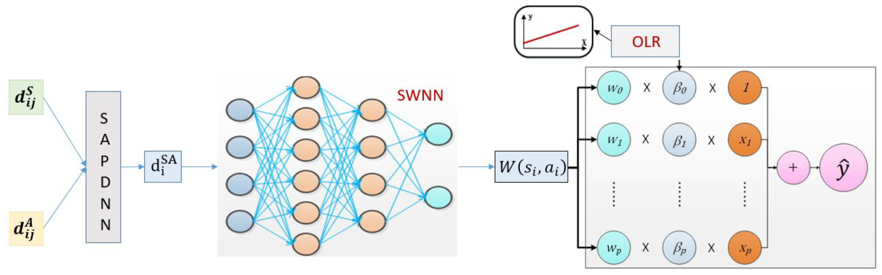
For the two sample points 𝑖 and 𝑗 in the space, it is assumed that there is a nonlinear fusion function ${\mathit{d}}_{\mathit{i}\mathit{j}}^{\mathit{S}\mathit{A}}$, that expresses a unified distance metric that takes into account both spatial distance and attribute distance; the expression is as follows:

$${\mathit{d}}_{\mathit{i}\mathit{j}}^{\mathit{S}\mathit{A}}={\mathit{f}}_{\mathit{p}\mathit{r}\mathit{o}\mathit{x}\mathit{i}\mathit{m}\mathit{i}\mathit{t}\mathit{y}}^{\mathit{S}\mathit{A}}\left({\mathit{d}}_{\mathit{i}\mathit{j}}^{\mathit{S}}, {\mathit{d}}_{\mathit{i}\mathit{j}}^{\mathit{A}}\right)$$

(4)

We proposed the spatial-attribute proximities neural network (SAPNN) to fit this function ${\mathit{d}}_{\mathit{i}\mathit{j}}^{\mathit{S}\mathit{A}}$. The network structure is shown in Figure 2:

SAPNN uses spatial distance and attribute distance as input and uses several dense layers for computation. Finally, we obtained the “spatial-attribute” unified distance between the two sample points i and j; the expression is as follows:

$${\mathit{d}}_{\mathit{i}\mathit{j}}^{\mathit{S}\mathit{A}}=\mathit{S}\mathit{A}\mathit{P}\mathit{N}\mathit{N}\left({\mathit{d}}_{\mathit{i}\mathit{j}}^{\mathit{S}},{\mathit{d}}_{\mathit{i}\mathit{j}}^{\mathit{A}}\right)$$

(5)

For any sample point 𝑖, the spatial distance vector $\left({\mathit{d}}_{\mathit{i}\mathbf{1}}^{\mathit{S}},{\mathit{d}}_{\mathit{i}\mathbf{2}}^{\mathit{S}},\dots ,{\mathit{d}}_{\mathit{i}\mathit{n}}^{\mathit{S}}\right)$ and the attribute distance vector $\left({\mathit{d}}_{\mathit{i}\mathbf{1}}^{\mathit{A}},{\mathit{d}}_{\mathit{i}\mathbf{2}}^{\mathit{A}},\dots ,{\mathit{d}}_{\mathit{i}\mathit{n}}^{\mathit{A}}\right)$ between 𝑖 and any other sample point can be obtained, n is the total number of sample points. For simplicity, the above two vectors can be abbreviated as ${\mathit{d}}_{\mathit{i}}^{\mathit{S}}$ and ${\mathit{d}}_{\mathit{i}}^{\mathit{A}}$.

Furthermore, considering the interaction of “spatial-attribute” unified distance metric between any two sample points in the point set, we proposed the spatial-attribute proximities deep neural network (SAPDNN) to obtain a new unified distance metric of the relationship between one point and all other points, the structure of SAPDNN is shown as Figure 3. First, we used SAPNN to obtain the unified distance between 𝑖 and any one point, the vector we obtained is $\left({\mathit{d}}_{\mathit{i}\mathbf{1}}^{\mathit{S}\mathit{A}},{\mathit{d}}_{\mathit{i}\mathbf{2}}^{\mathit{S}\mathit{A}},\dots ,{\mathit{d}}_{\mathit{i}\mathit{n}}^{\mathit{S}\mathit{A}}\right)$. Then, the vector undergoes several dense layers for nonlinear fusion. Finally, we obtained the unified distance metric ${\mathit{d}}_{\mathit{i}}^{\mathit{S}\mathit{A}}$, which can characterize the unified distance metric of spatial feature and attribute feature between the sample point 𝑖 and all other sample points in the space. The expression is as follows:

$${\mathit{d}}_{\mathit{i}}^{\mathit{S}\mathit{A}}=\mathit{S}\mathit{A}\mathit{P}\mathit{D}\mathit{N}\mathit{N} \left({\mathit{d}}_{\mathit{i}}^{\mathit{S}},{\mathit{d}}_{\mathit{i}}^{\mathit{A}}\right)$$

(6)

It is worth pointing out that SAPDNN can adjust the model input, model structure and number of neurons according to the research situation. It can input two or more kinds of neighbor relationships for neural network fusion operation, and it can easily extend the fusion of neighbor relationships to other new feature scales. In this section, the neighbor relationships we aggregated are the spatial relationship and attribute relationships.

3.2. SANNWR Model

3.2.1. The Definition of SANNWR Model

In order to estimate spatial non-stationarity accurately, the GNNWR model was modified by using the “spatial-attribute” unified distance metric which takes attribute features into account. We proposed the spatial and attribute neural network-weighted regression (SANNWR) model, the mathematical expression is as follows:

$$\mathit{y}\left({\mathit{s}}_{\mathit{i}},{\mathit{a}}_{\mathit{i}}\right)={\mathit{\beta }}_{\mathbf{0}}\left({\mathit{s}}_{\mathit{i}},{\mathit{a}}_{\mathit{i}}\right)+{\displaystyle \sum }_{\mathit{k}=\mathbf{1}}^{\mathit{p}}{\mathit{\beta }}_{\mathit{k}}\left({\mathit{s}}_{\mathit{i}},{\mathit{a}}_{\mathit{i}}\right){\mathit{x}}_{\mathit{i}\mathit{k}}+{\mathit{\epsilon }}_{\mathit{i}} \mathit{i}=\mathbf{1},\mathbf{2},\cdots ,\mathit{n}$$

(7)

The regression coefficient ${\mathit{\beta }}_{\mathit{k}}$ is a function of spatial feature and attribute feature, ${\mathit{s}}_{\mathit{i}}$ is the spatial feature at coordinate point $\left({\mathit{u}}_{\mathit{i}},{\mathit{v}}_{\mathit{i}}\right)$, ${\mathit{a}}_{\mathit{i}}$ is the attribute feature at coordinate point $\left({\mathit{u}}_{\mathit{i}},{\mathit{v}}_{\mathit{i}}\right)$. We can use ${\mathit{w}}_{\mathit{k}}\left({\mathit{s}}_{\mathit{i}},{\mathit{a}}_{\mathit{i}}\right)$ to indicate the weight of the coefficient of the ith sample point, ${\mathit{\beta }}_{\mathit{k}}\left({\mathit{s}}_{\mathit{i}},{\mathit{a}}_{\mathit{i}}\right)$ in GWR can be expressed as ${\mathit{\beta }}_{\mathit{k}}\left({\mathit{s}}_{\mathit{i}},{\mathit{a}}_{\mathit{i}}\right)={\mathit{w}}_{\mathit{k}}\left({\mathit{s}}_{\mathit{i}},{\mathit{a}}_{\mathit{i}}\right)\times {\widehat{\mathit{\beta }}}_{\mathit{k}}\left(\mathit{O}\mathit{L}\mathit{R}\right)$. Substitute this formula, $\mathit{y}\left({\mathit{s}}_{\mathit{i}},{\mathit{a}}_{\mathit{i}}\right)$ can be updated as:

$$\widehat{\mathit{y}}\left({\mathit{s}}_{\mathit{i}},{\mathit{a}}_{\mathit{i}}\right)={\displaystyle \sum }_{\mathit{k}=\mathbf{0}}^{\mathit{p}}{\widehat{\mathit{\beta }}}_{\mathit{k}}\left({\mathit{s}}_{\mathit{i}},{\mathit{a}}_{\mathit{i}}\right){\mathit{x}}_{\mathit{i}\mathit{k}}={\displaystyle \sum }_{\mathit{k}=\mathbf{0}}^{\mathit{p}}{\mathit{w}}_{\mathit{k}}\left({\mathit{s}}_{\mathit{i}},{\mathit{a}}_{\mathit{i}}\right)\times {\widehat{\mathit{\beta }}}_{\mathit{k}}\left(\mathit{O}\mathit{L}\mathit{R}\right){\mathit{x}}_{\mathit{i}\mathit{k}}$$

(8)

The solution of the model can be expressed as the following matrix form:

$$\widehat{\mathit{y}}\left({\mathit{s}}_{\mathit{i}},{\mathit{a}}_{\mathit{i}}\right)={\mathit{x}}_{\mathit{i}}^{\mathit{T}}\widehat{\mathit{\beta }}\left({\mathit{s}}_{\mathit{i}},{\mathit{a}}_{\mathit{i}}\right)={\mathit{x}}_{\mathit{i}}^{\mathit{T}}\mathit{W}\left({\mathit{s}}_{\mathit{i}},{\mathit{a}}_{\mathit{i}}\right){({\mathit{X}}^{\mathit{T}}\mathit{X})}^{-\mathbf{1}}{\mathit{X}}^{\mathit{T}}\mathit{y}$$

(9)

$\mathit{W}\left({\mathit{s}}_{\mathit{i}},{\mathit{a}}_{\mathit{i}}\right)$ is a unified distance weight matrix which reflects spatial non-stationarity in geographical relations, the weight is related to the space distance ${\mathit{s}}_{\mathit{i}}$ of the ith point and the attribute distance ${\mathit{a}}_{\mathit{i}}$ of the ith point. The mathematical expression is as follows:

$$\mathit{W}\left({\mathit{s}}_{\mathit{i}},{\mathit{a}}_{\mathit{i}}\right)=\left[\begin{array}{cccc}{\mathit{w}}_{\mathbf{0}}\left({\mathit{s}}_{\mathit{i}},{\mathit{a}}_{\mathit{i}}\right)& \mathbf{0}& \mathbf{0}& \mathbf{0}\\ \mathbf{0}& {\mathit{w}}_{\mathbf{1}}\left({\mathit{s}}_{\mathit{i}},{\mathit{a}}_{\mathit{i}}\right)& \mathbf{0}& \mathbf{0}\\ \mathbf{0}& \mathbf{0}& \dots & \mathbf{0}\\ \mathbf{0}& \mathbf{0}& \mathbf{0}& {\mathit{w}}_{\mathit{p}}\left({\mathit{s}}_{\mathit{i}},{\mathit{a}}_{\mathit{i}}\right)\end{array}\right]$$

(10)

The measure of spatial non-stationarity is actually determined by $\mathit{W}\left({\mathit{s}}_{\mathit{i}},{\mathit{a}}_{\mathit{i}}\right),$ and $\mathit{W}\left({\mathit{s}}_{\mathit{i}},{\mathit{a}}_{\mathit{i}}\right)$is determined by the spatial distance and the attribute distance. We used SAPDNN to merge spatial distance and attribute distance, so that a unified metric of “spatial-attribute” distance could be obtained. Therefore, $\mathit{W}\left({\mathit{s}}_{\mathit{i}},{\mathit{a}}_{\mathit{i}}\right)$ is a function of ${\mathit{d}}_{\mathit{i}}^{\mathit{S}\mathit{A}}$ and can be expressed as:

$$\mathit{W}\left({\mathit{s}}_{\mathit{i}},{\mathit{a}}_{\mathit{i}}\right)={\mathit{f}}_{\mathit{k}\mathit{e}\mathit{r}\mathit{n}\mathit{e}\mathit{l}}\left({\mathit{d}}_{\mathit{i}}^{\mathit{S}\mathit{A}}\right)={\mathit{f}}_{\mathit{k}\mathit{e}\mathit{r}\mathit{n}\mathit{e}\mathit{l}}\left(\mathit{S}\mathit{A}\mathit{P}\mathit{D}\mathit{N}\mathit{N}\left({\mathit{d}}_{\mathit{i}}^{\mathit{S}},{\mathit{d}}_{\mathit{i}}^{\mathit{A}}\right)\right)$$

(11)

In this formula, ${\mathit{f}}_{\mathit{k}\mathit{e}\mathit{r}\mathit{n}\mathit{e}\mathit{l}}$ represents a weight kernel function in a generalized sense, ${\mathit{d}}_{\mathit{i}}^{\mathit{S}}$ can be obtained by using Euclidean or non-Euclidean spatial distance metrics, ${\mathit{d}}_{\mathit{i}}^{\mathit{A}}$ can be obtained according to the attribute distance measurement method defined in 3.1.2 above.

The SANNWR model was based on the GNNWR model and integrated SAPDNN to realize the fusion of spatial distance and attribute distance. In contrast to GNNWR, SANNWR uses a unified distance metric in the modeling process. It can more accurately reflect the relationship between each sample point and realize the exact solution of spatial non-stationarity. The implementation process is shown as follows:(Figure 4).

First, we used SAPDNN to obtain the unified distance vector ${\mathit{d}}_{\mathit{i}}^{\mathit{S}\mathit{A}}$, then took this vector as input to the SWNN to solve the weight matrix $\mathit{W}\left({\mathit{s}}_{\mathit{i}},{\mathit{a}}_{\mathit{i}}\right)$; the solution process of this matrix can be expressed as:

$$\mathit{W}\left({\mathit{s}}_{\mathit{i}},{\mathit{a}}_{\mathit{i}}\right)=\mathit{S}\mathit{W}\mathit{N}\mathit{N}\left({\mathit{d}}_{\mathit{i}}^{\mathit{S}\mathit{A}}\right)=\mathit{S}\mathit{W}\mathit{N}\mathit{N}\left(\mathit{S}\mathit{T}\mathit{A}\mathit{P}\mathit{D}\mathit{N}\mathit{N}\left({\mathit{d}}_{\mathit{i}}^{\mathit{S}},{\mathit{d}}_{\mathit{i}}^{\mathit{A}}\right)\right)$$

(12)

The fit value $\widehat{\mathit{y}}$ can be expressed as:

$$\widehat{\mathit{y}}=\left[\begin{array}{c}\begin{array}{c}{\mathit{s}}_{\mathbf{1}}\\ {\mathit{s}}_{\mathbf{2}}\end{array}\\ \dots \\ {\mathit{s}}_{\mathit{n}}\end{array}\right]=\left[\begin{array}{c}\begin{array}{c}{\mathit{x}}_{\mathbf{1}}^{\mathit{T}}\mathit{W}\left({\mathit{s}}_{\mathbf{1}},{\mathit{a}}_{\mathbf{1}}\right){\left({\mathit{X}}^{\mathit{T}}\mathit{X}\right)}^{-\mathbf{1}}{\mathit{X}}^{\mathit{T}}\\ {\mathit{x}}_{\mathbf{2}}^{\mathit{T}}\mathit{W}\left({\mathit{s}}_{\mathbf{2}},{\mathit{a}}_{\mathbf{2}}\right){\left({\mathit{X}}^{\mathit{T}}\mathit{X}\right)}^{-\mathbf{1}}{\mathit{X}}^{\mathit{T}}\end{array}\\ \dots \\ {\mathit{x}}_{\mathit{n}}^{\mathit{T}}\mathit{W}\left({\mathit{s}}_{\mathit{n}},{\mathit{a}}_{\mathit{n}}\right){\left({\mathit{X}}^{\mathit{T}}\mathit{X}\right)}^{-\mathbf{1}}{\mathit{X}}^{\mathit{T}}\end{array}\right]\mathit{y}={\mathit{S}}_{\mathit{S}\mathit{A}\mathit{N}\mathit{N}\mathit{W}\mathit{R}}\mathit{y}$$

(13)

In this formula, ${\mathit{S}}_{\mathit{S}\mathit{A}\mathit{N}\mathit{N}\mathit{W}\mathit{R}}$ is the hat matrix of the SANNWR model.

3.2.2. Model Structure and Parameters

SANNWR consists of SAPDNN and SWNN. SAPDNN is composed of three layers: input layer, a hidden layer, and an output layer, which are connected in full connection mode. The SWNN has four layers of network structure, including two hidden layers, one for input and one for output. The unified distance is input into SWNN, and the weight matrix of the independent variables of fitting points is output [25]. All the layers in SWNN are connected in full connection mode. The neural network adopts a fully connected layer and dropout technologies to enhance the generalization capability, as suggested by Srivastava et al. (2014) [26].

The structure of SANNWR model is shown as Figure 5:

The super parameter settings of SANNWR model is listed in

Table 2. The super parameter settings of SANNWR.

SANNWR Model Structure Setup
Hierarchy		Settings	Input Data Dimension	Output Data Dimension
SAPDNN
Input layer		-	2	2
Hidden layer		3	2	3
Output layer		1	3	1
SWNN
Input layer		-	1120	1120
Hidden layer-a		50	1120	50
Hidden layer-b		20	50	20
Output layer		7	20	7
SANNWR Model hyper-parameter setting
Initial Learning Rate	Max Learning Rate	Maximum value of epoch	Batch size	Dropout
0.02	0.67	200,000	16	0.7

as follows:

3.2.3. Model Optimization Training

The accuracy of the fitting value ${\widehat{\mathit{y}}}_{\mathit{i}}$ depends on the degree of fitting the proximity relationship between sample points by SAPDNN network and the degree of fitting the nonlinear relationship by SWNN network. The following figure shows the training process from the initial spatial distance and attribute distance to the final weight matrix.

In order to obtain a better training effect, dropout technology was used to enhance the generalization ability of the model (Figure 6). The dropout technique randomly invalidates some nodes in the neural network during the training process to reduce the complexity of the model. This technique can reduce the overfitting and improve the generalization of the model. He-parameter initialization and PReLU activation function are used to improve the optimization efficiency of the model. At the same time, the batch normalization technique and the gradient descent method with variable learning rate are adopted to further improve the computing ability of the model. In addition, early stop method is used to prevent deep neural network overfitting. The training process is listed in

Table 3. The training process of SANNWR.

SANNWR Model Training and Optimization Process

1: Neural network model training starts; 2: Divide dataset. The data set is divided into a cross-validation set and a test set. Then, the cross-validation set is divided into N equal parts. When we train the model, one part of the cross-validation set is used as the verification set and the rest are used as the training set. 3: Initialize the neural network hyper-parameters according to the preset related parameters, including initial and maximum learning rate, iteration times, etc. 4: Divide the training set into multiple mini batches. 5: Use mini-batch as input in sequence 6: Check whether the current epoch is complete. If not, switch to the next Mini Batch for training. 7: Calculate the overfitting index for the completed epoch. 8: View training indicators of the current epoch. If it is better than the previous optimal model, record the current neural network parameters and zero the tolerance value. Otherwise, judging whether the tolerance value has reached the maximum value; If yes, end training and restore parameters of the optimal model; Otherwise, increasing the tolerance value to continue training; 9: Check whether the number of epoch times has reached the upper limit. If yes, end training and restore parameters of the optimal model; If not, scramble the data set involved in the training, and continue the training. 10: Calculate and verify the generalization capability of the model. 11: End the neural network training process.

.

4. Results

4.1. Design of Experiment

The dataset used in this paper was obtained from the annual average data of PM₂.₅ concentration monitoring stations in China in 2018, which includes a total of 1465 monitoring stations. PM₂.₅ concentration monitoring stations have many attribute features, including aerosol (AOD), 2 m temperature (TEMP), relative humidity (r), precipitation (TP), 10 m wind speed (WS), and elevation (DEM). In this paper, wind direction (WD) data were selected as the measure of attribute distance. In terms of model selection, this paper chose the GWR, GNNWR and SANNWR models for comparison. In order to verify the effectiveness of the “spatial-attribute” unified distance metric, GWR and GSNNWR models compared the spatial distance and attribute distance, respectively, while the SANNWR model used the unified distance metric as the measurement method.

Kernel function is a kind of mapping function for the nonlinear mapping of data, and is often used in statistics. According to the different spatial kernel functions, the GWR model can be combined in many ways. The fixed kernel function uses a fixed mapping mode for all the inputs, and the adaptive kernel function adjusts the weight of the mapping according to the distribution of the input data. To fully compare the performance differences between the models, we chose the fixed and adaptive kernel functions combined with Gaussian and Bi-square kernel functions, and select the more commonly used AICc criterion in the optimization criterion. It should be noted that the spatial distribution of stations in China is dense in the east and sparse in the west, which will lead to the lower reliability of the kernel function of the combination of fixed and bi-square (Nakaya, 2014) [27]. Therefore, this chapter does not consider the use of this kernel function combination. The specific kernel function combination settings of the GWR model are shown in

Table 4. Specific Kernel Function Combination Settings for GWR Models.

Combination Name	Kernel Function Type	kernel Function Structure
GWR-AFG	Fixed	Gaussian
GWR-AAG	adaptive	Gaussian
GWR-AAB	adaptive	Bi-square

.

Table 5. Software and hardware environment of these models.

Model Name	GWR	GNNWR and SANNWR
Software environment	MATLAB 2016a	TensorFlow 1.7/CUDA9.0/ Python 3.6
Number of machines	1
Hardware environment	CPU: Inter(R) XEON E3-1231V3 3.4 GHz Memory: 32 GB Graphics card: NVIDIA Quadro RTX4000 OS: Windows 10 ×64

lists the modeling environment. The GWR modeling process is implemented based on MATLAB 2016a software. The optimal GWR model is solved by fminbnd function. GNNWR and SANNWR are implemented based on Python 3.6, CUDA9.0, and TensorFlow 1.7.

4.2. Analysis of Experimental Results

The GWR, GNNWR, and SANNWR models were cross-validated with ten-fold cross-validations. In addition to SANNWR, GWR and GNNWR were modeled using spatial distance (represented by letter S) and attribute distance (represented by letter A), respectively. Finally, six GWR modeling methods, two GNNWR modeling methods and the SANNWR model were compared. The evaluation indexes included R², RMSE, MAE, MAPE and AICc. The results of the training set and the verification set are the average values of the cross-validation results. The F₁ test results of each model show that the significance level is 0.01, which proves that there is significant spatial non-stationarity among atmospheric environmental pollutants in China.

The experimental results are shown in

Table 6. Average value of the ten cross-validation results of the training set.

Model	Ten Cross-Validation Results (Fitness)											Evaluation Result (Forecast)
	Train Set							Validation Set				Test Set
	R2	RMSE	MAE	MAPE	AICc	F1	p-Value	R2	RMSE	MAE	MAPE	R2	RMSE	MAE	MAPE
GWR-AAB-A	0.693	7.375	5.625	15.568%	7769.641	0.666	0.01	0.665	7.755	6.049	15.719%	0.724	8.456	5.704	14.373%
GWR-AFG-A	0.692	7.378	5.607	15.475%	7779.451	0.671	0.01	0.687	7.490	5.869	15.381%	0.721	8.494	5.809	14.566%
GWR-AAG-A	0.699	7.299	5.583	15.511%	7764.819	0.654	0.01	0.648	7.934	6.212	16.364%	0.711	8.438	6.526	17.640%
GWR-AAB-S	0.711	7.175	5.437	15.210%	7656.975	0.615	0.01	0.737	6.871	5.342	14.256%	0.739	8.190	5.741	15.098%
GWR-AFG-S	0.708	7.221	5.603	15.326%	7678.801	0.626	0.01	0.719	7.152	5.598	14.624%	0.781	7.624	5.900	15.555%
GWR-AAG-S	0.710	7.191	5.364	15.239%	7666.507	0.616	0.01	0.642	8.005	6.268	16.533%	0.742	7.979	5.982	15.929%
GNNWR-A	0.714	7.064	5.362	14.698%	7588.525	0.137	0.01	0.706	7.697	5.541	15.994%	0.739	8.237	5.487	13.703%
GNNWR-S	0.841	5.270	3.866	10.773%	6912.113	0.278	0.01	0.768	6.387	4.668	12.565%	0.844	6.377	4.307	11.213%
SANNWR	0.860	4.981	3.651	10.142%	6792.544	0.248	0.01	0.824	5.747	4.261	10.845%	0.857	6.251	4.205	10.949%

. The GWR model and GNNWR model take spatial distance and attribute distance as inputs, respectively. The performance of the model using attribute distance is lower than the model using spatial distance, which proves that the attribute distance alone does not improve the fitting performance of the model. Comparing three GWR models using spatial distance metric, we can see that the fitting ability of the GWR-AFG-S model is slightly worse, the GWR-AAB-S model is slightly better than the GWR-AAG-S model in terms of R², RMSE, MAPE, and AICc, but slightly worse in terms of MAE. The results show that the spatial modeling capability of the two methods is equivalent. Comparing the GNNWR-S model with the GWR-AAB-S model, the indicators are as follows: R² (0.841 vs. 0.711), RMSE (5.270 vs. 7.175), MAE (3.866 vs. 5.437), MAPE (10.773% vs. 15.210%), AICc (6912.113 vs. 7656.975). According to the above five indexes, the GNNWR-S model is better than the GWR-AAB-S model, which indicates that the GNNWR model has a better fitting ability than the GWR model. Furthermore, the SANNWR model outperforms the GNNWR model in terms of various indicators and becomes the model with the best fit performance among the nine modeling methods. It also proves that the “spatial-attribute” unified distance metric can better reflect the interrelationship between sample points and improve the analytical capability of the model for spatial non-stationarity.

In addition, we used a test set to examine the predictive effect and generalization ability of these models. As shown in Table 6, on the test set, the R², RMSE, MAE and MAPE evaluation indexes of SANNWR model are better than those of the GWR and GNNWR models, indicating that the SANNWR model has better generalization capability.

In order to further reveal the fitting ability of these models, the scatter plots of the fitted values and true values of the GWR, GNNWR and SANNWR models are presented. In the scatter plots, the abscissa is the observed value, the ordinate is the estimated value, and the color of point indicates the number of data. The fitted lines for all points are drawn and the angle between the diagonal line and the fitted line reflects the similarity of the fitting. In the fitting effect presentation part, the cross-validated validation set of each model are used to draw these charts, the data volume is the same as that of the cross-validation set, so it is more convincing. The result is shown as follows:

As can be seen from Figure 7, the point distribution of the GWR model is rather scattered and the distribution of GNNWR and SANNWR points is relatively centralized, it means that the GWR model shows the worst fitting ability. Then, comparing the GNNWR and SANNWR, the scatter points of SANNWR are more concentrated, the angle between the scatter points fitting line and the 1:1 line is the smallest, which indicates that the SANNWR model has a better fitting ability than the GNNWR model. We can obtain the same conclusion from the values of MAE, MAPE, and RMSE.

Figure 8 shows the scatter chart of each model in the test set to show the prediction capability of these models. The result is similar to the scatter chart of the training set. The GWR model has the worst prediction accuracy. The GNNWR model has similar results to SANNWR model, but slightly weaker.

5. Discussion

More and more researchers use attribute features in spatial prediction, including the prediction of element concentrations, loss on ignition, and pH in the soils of south west England using high resolution remote sensing and geophysical survey data (Kirkwood C, Cave M and Beamish D, 2016) [28], and a study of multiple machine learning models on Walker Lake datasets (Ahmed W, Muhammad K, Glass H J, 2022) [29]. These studies have chosen to use machine learning to process data. In the big data era, the fine granularity and precision of geographical data are greatly improved, and the interrelationship detection between geographical elements becomes more refined. The original expression of proximity is difficult to meet the need of spatial non-stationarity analysis, and the complexity of spatial proximity expression needs to be improved urgently. So, the neural network is introduced to fit the complex spatial non-stationarity process. In addition to dealing with massive data in a single dimension, the neural network can calculate the data in different dimensions and obtain the optimal weight of the data in different dimensions independently during the training process. We introduced data from the attribute dimension based on the spatial dimension, which improved the fitting accuracy compared with the single dimension. In the future, we can extend the method to the time dimension, and we believe that the method can achieve better results.

Our experiment only combined spatial distance and a single attribute, this method has many research directions, such as multi-attribute distance using different measurement formulas, multi-attribute fusion.

6. Conclusions

In this study, we combined a spatial feature with a single attribute feature, defined a unified distance metric form of spatial distance and attribute distance, and proposed SAPDNN for nonlinear fusion of spatial distance and attribute distance. Then, we upgraded the GNNWR with the “spatial -attribute” unified distance metric and proposed the spatial and attribute neural network-weighted regression (SANNWR) model. On this basis, we conducted a case study. In our case, the spatial non-stationarity model was conducted with a PM₂.₅ concentration and other atmospheric environmental factors in China. The fitting effect and prediction ability of SANNWR were compared and analyzed with GWR and GNNWR models, with the results summarized as follows: in terms of the choice of the distance metric, single attribute distance is less effective than single spatial distance and unified distance can represent more semantic information. From the results of the comparison of the models, the SANNWR model has a significantly better fitting ability and generalization ability than the GWR model, and has some advantages over the GNNWR model. In Table 6, the GNNWR-A, the GNNWR-S, and the SANNWR can be considered as the same regression fitting network (SWNN + OLR) receiving three different inputs: a single attribute distance, a single spatial distance, and a fusion distance. For the regression fitting network (SWNN + OLR), the model structure and training method were the same. Therefore, the precision difference was caused by the information carried in the input data. The result of fusion distance was better than that of single spatial distance or single attribute distance. Results showed that the fusion distance has more effective information, and this fusion distance is obtained by the SAPDNN, which combined the space distance and the attribute distance. Our comparison results on the test dataset were consistent with the training set and the validation set, which indicates that the model did not overfit.

The results showed that the “spatial-attribute” unified distance metric can not only reveal the relationship between geographical elements more precisely, but also improve the fitting effect and generalization ability of the model to the spatial non-stationary elements. It also proved that the SANNWR model has strong fitting ability and generalization ability.

References

1. Cressie, N. Statistics for spatial data. Terra Nova 1992, 4, 613–617. [Google Scholar] [CrossRef]
2. Cressie, N.; Wikle, C.K. Statistics for Spatio-Temporal Data; John Wiley & Sons: New York, NY, USA, 2015; ISBN 978-047-169-274-4. [Google Scholar]
3. Fotheringham, A.S.; Crespo, R.; Yao, J. Geographical and temporal weighted regression (GTWR). Geogr. Anal. 2015, 47, 431–452. [Google Scholar] [CrossRef] [Green Version]
4. Goodchild, M.F. Prospects for a space–time GIS: Space–time integration in geography and GIScience. Ann. Assoc. Am. Geogr. 2013, 103, 1072–1077. [Google Scholar] [CrossRef]
5. Brunsdon, C.; Fotheringham, A.S.; Charlton, M.E. Geographically weighted regression: A method for exploring spatial nonstationarity. Geogr. Anal. 1996, 28, 281–298. [Google Scholar] [CrossRef]
6. Xu, B.; Lin, B. Factors affecting CO2 emissions in China’s agriculture sector: Evidence from geographically weighted regression model. Energy Policy 2017, 104, 404–414. [Google Scholar] [CrossRef]
7. Cahill, M.; Mulligan, G. Using geographically weighted regression to explore local crime patterns. Soc. Sci. Comput. Rev. 2007, 25, 174–193. [Google Scholar] [CrossRef]
8. Sheng, J.; Han, X.; Zhou, H. Spatially varying patterns of afforestation/reforestation and socio-economic factors in China: A geographically weighted regression approach. J. Clean. Prod. 2017, 153, 362–371. [Google Scholar] [CrossRef]
9. Huang, B.; Wu, B.; Barry, M. Geographically and temporally weighted regression for modeling spatio-temporal variation in house prices. Int. J. Geogr. Inf. Sci. 2010, 24, 383–401. [Google Scholar] [CrossRef]
10. Wu, B.; Li, R.R.; Huang, B. A geographically and temporally weighted autoregressive model with application to housing prices. Int. J. Geogr. Inf. Sci. 2014, 28, 1186–1204. [Google Scholar] [CrossRef]
11. Fotheringham, A.S.; Crespo, R.; Yao, J. Exploring, modelling and predicting spatiotemporal variations in house prices. Ann. Reg. Sci. 2015, 54, 417–436. [Google Scholar] [CrossRef]
12. Yao, J.; Fotheringham, A.S. Local spatiotemporal modeling of house prices: A mixed model approach. Prof. Geogr. 2016, 68, 189–201. [Google Scholar] [CrossRef]
13. Brunsdon, C.; Fotheringham, S.; Charlton, M. Geographically weighted regression. J. R. Stat. Soc. Ser. D (Stat.) 1998, 47, 431–443. [Google Scholar] [CrossRef]
14. Fotheringham, A.S.; Brunsdon, C.; Charlton, M. Geographically Weighted Regression: The Analysis of Spatially Varying Relationships; John Wiley & Sons: Oxford, UK; New York, NY, USA, 2002; ISBN 978-661-027-017-0. [Google Scholar]
15. Gollini, I.; Lu, B.; Charlton, M. GWmodel: An R Package for Exploring Spatial Heterogeneity using Geographically Weighted Models. arXiv 2014. [Google Scholar] [CrossRef] [Green Version]
16. Fotheringham, A.S.; Yang, W.; Kang, W. Multiscale geographically weighted regression (MGWR). Ann. Am. Assoc. Geogr. 2017, 107, 1247–1265. [Google Scholar] [CrossRef]
17. Li, Z. Measuring bandwidth uncertainty in multiscale geographically weighted regression using akaike weights. Ann. Am. Assoc. Geogr. 2020, 110, 1500–1520. [Google Scholar] [CrossRef]
18. Yu, H. Inference in multiscale geographically weighted regression. Geogr. Anal. 2020, 52, 87–106. [Google Scholar] [CrossRef]
19. Yue, P.; Ramachandran, R.; Baumann, P. Recent activities in Earth data science [technical committees]. IEEE Geosci. Remote Sens. Mag. 2016, 4, 84–89. [Google Scholar] [CrossRef]
20. Yue, P.; Shangguan, B.; Hu, L. Towards a training data model for artificial intelligence in earth observation. Int. J. Geogr. Inf. Sci. 2022, 36, 2113–2137. [Google Scholar] [CrossRef]
21. Wu, S. The Theory and Method of Geographically and Temporally Neural Network Weighted Regression. Ph.D. Thesis, Zhejiang University, Hangzhou, China, 2018. [Google Scholar]
22. Wu, S. Modeling spatially anisotropic nonstationary processes in coastal environments based on a directional geographically neural network weighted regression. Sci. Total Environ. 2020, 709, 136097. [Google Scholar] [CrossRef]
23. Yue, P.; Di, L.; Wei, Y. Intelligent services for discovery of complex geospatial features from remote sensing imagery. ISPRS J. Photogramm. Remote Sens. 2013, 83, 151–164. [Google Scholar] [CrossRef]
24. Shi, H.; Zhang, L.; Liu, J. A new spatial-attribute weighting function for geographically weighted regression. Can. J. For. Res. 2006, 36, 996–1005. [Google Scholar] [CrossRef] [Green Version]
25. Du, Z.; Wang, Z.; Wu, S. Geographically neural network weighted regression for the accurate estimation of spatial non-stationarity. Int. J. Geogr. Inf. Sci. 2020, 34, 1353–1377. [Google Scholar] [CrossRef]
26. Srivastava, N. Dropout: A simple way to prevent neural networks from overfitting. J. Mach. Learn. Res. 2014, 15, 1929–1958. [Google Scholar] [CrossRef]
27. Nakaya, T. GWR4 User Manual. WWW Document. 2014. Available online: http://www. st-andrews.ac.uk/geoinformatics/wp-content/uploads/GWR4manual_201311.pdf (accessed on 4 November 2013).
28. Kirkwood, C.; Cave, M.; Beamish, D.; Grebby, S.; Ferreira, A. A machine learning approach to geochemical mapping. J. Geochem. Explor. 2016, 167, 49–61. [Google Scholar] [CrossRef] [Green Version]
29. Ahmed, W.; Muhammad, K.; Glass, H.J.; Chatterjee, S.; Khan, A.; Hussain, A. Novel MLR-RF-Based Geospatial Techniques: A Comparison with OK. ISPRS Int. J. Geo-Inf. 2022, 11, 371. [Google Scholar] [CrossRef]
Figure 1. Study area.
Ijgi 11 00620 g001
Figure 2. The structure of SAPNN.
Ijgi 11 00620 g002
Figure 3. The structure of SAPDNN.
Ijgi 11 00620 g003
Figure 4. The modeling process of SANNWR.
Ijgi 11 00620 g004
Figure 5. The structure of SANNWR.
Ijgi 11 00620 g005
Figure 6. The training process of SANNWR.
Ijgi 11 00620 g006
Figure 7. Scatter plots of predicted and actual values in the validation set.
Ijgi 11 00620 g007
Figure 8. Scatter plots of predicted and actual values in the test set.
Ijgi 11 00620 g008