Article

Different Ways Ambient and Immobile Population Distributions Influence Urban Crime Patterns

by
Natalia Sypion-Dutkowska
1,
Minxuan Lan
2,3,*,
Marek Dutkowski
1 and
Victoria Williams
4
1
Institute of Spatial Management and Socioeconomic Geography, University of Szczecin, Mickiewicza 64 Street, 71-101 Szczecin, Poland
2
Department of Geography and Planning, The University of Toledo, Toledo, OH 43606, USA
3
Department of Justice Sciences, The University of Findlay, Findlay, OH 45840, USA
4
Department of Behavioral Sciences, The University of Findlay, Findlay, OH 45840, USA
*
Author to whom correspondence should be addressed.
ISPRS Int. J. Geo-Inf. 2022, 11(12), 581; https://doi.org/10.3390/ijgi11120581
Submission received: 11 August 2022 / Revised: 10 October 2022 / Accepted: 19 November 2022 / Published: 22 November 2022
(This article belongs to the Special Issue Urban Geospatial Analytics Based on Crowdsourced Data)

Abstract

:
The article aims to propose a new way of estimating the ambient and immobile urban population using geotagged tweets and age structure, and to test how they are related to urban crime patterns. Using geotagged tweets and age structure data in 37 neighborhoods of Szczecin, Poland, we analyzed the following crime types that occurred during 2015–2017: burglary in commercial buildings, drug crime, fight and battery, property damage, and theft. Using negative binomial regression models, we found a positive correlation between the size of the ambient population and all investigated crime types. Additionally, neighborhoods with more immobile populations (younger than 16 or older than 65) tend to experience more commercial burglaries, but not other crime types. This may be related to the urban structure of Szczecin, Poland. Neighborhoods with higher rates of poverty and unemployment tend to experience more commercial burglaries, drug problems, property damage, and thefts. Additionally, the count of liquor stores is positively related to drug crime, fight-battery, and theft. This article suggests that the age structure of the population has an influence on the distribution of crime, thus it is necessary to tailor crime prevention strategies for different areas of the city.

1. Introduction

Each crime incident is geographic in nature. It is committed at a certain place and time. The offender usually comes to the place of his/her commission from other places, and he/she also has a permanent or the most frequent place of residence, e.g., a place of residence, work, or study [1]. These places may be identical or adjacent to each other. Time and place play fundamental roles in understanding and explaining crime patterns. The spatiotemporal differentiation is one of the distinctions of crime pattern studies and a premise for research on this issue. In order to study crime patterns, various efforts have been made by scholars not only in criminology, but also geography, sociology, and social sciences at large. Geography of crime in the geography field and environmental criminology (also known as crime science) in the criminology field specifically focus on the location of crime incidents.
Theories from environmental criminology are helpful in understanding temporal and spatial crime patterns. The routine activity theory argues that crime is the result of the direct contact of three elements in space and time: a motivated offender, a suitable target, and the absence of the capable guardian [2,3]. It suggests that the people’s routine activities contribute to possible intersections in time and space with a potential offender, and when it happens, the probability of crime increases drastically [2].
Crime pattern theory also shows that the distribution of population in time and space is important to crime pattern studies. This theory suggests that the locations of crime incidents are not accidental, rather, they have clear spatio-temporal patterns. This theory highlights the activity spaces and routes connecting them. These activity spaces include (1) nodes–e.g., residences, shopping centers, workplaces, schools, recreation and entertainment areas, places to meet friends, etc., (2) paths connecting these nodes, and (3) edges, which are boundaries dividing areas with various forms of management, rulership, or functions. Moving along the paths between the nodes, the criminal’s awareness spaces are created. The space of action is reflected in the offender’s consciousness in the form of a cognitive space map. According to this theory, a motivated offender has contact with a relatively small part of the city areas in the course of routine everyday activities. From perceived and realized nodes, paths, and edges, he/she selects appropriate objects or victims of crime in a multi-stage decision-making process. The distribution of crime in a city depends on its spatial structure, transport system, and street networks, and is shaped by the distribution of crime generators, attractors, and detractors [1,4]. Moreover, the city crime problem usually concentrates in relatively small areas, as the Law of Crime Concentration and Iron Law of Troublesome Places suggest [5,6,7,8,9]. In many cities, the downtown area or central business districts would fall in this category because of the concentration of population and opportunities.
Thus, the problem of obtaining information about the real-time or close-to-real-time location of the population is one of the key pieces of information in crime pattern research. Publicly available census information does not reflect the actual whereabouts of the population as it does not take into account the phenomenon of daily movements of the citizens [10]. As many studies have pointed out, increased mobility and mobile range can change the dynamic distribution of the population, which in turn, influences the crime pattern [11,12,13,14,15]. Such a population measure issue can be even more acute when using it to measure crime and other socioeconomic factors. One frequently used crime indicator is the crime rate, which is calculated by dividing the number of recorded crimes in a certain area by the population of that area. Similar indicators are practically used in various socioeconomic phenomena studies, e.g., GDP per capita, poverty rate, unemployment rate, etc. However, there are also problems when determining the actual residing population. For large areas, such as countries or regions, census data are generally taken every 10 years. Such censuses are not always available in all regions, and the census data can become obsolete because of the long measure gap, which could distort the results. Data from the current population registration kept by the government are commonly used in such studies, especially in European countries. Their credibility depends on the quality of administration and the provisions of the registration obligation. Considerable migratory movements, especially periodic residents like college students, tourists, and those on business trips, further make it difficult to determine the actual residing population. In countries with weak administration and a low level of civil discipline, such registers are not kept, and the count of actually residing population can only be estimated.
The above-stated data quality concerns may also influence smaller areas, such as cities and their neighborhoods. Thus, the emerging measures which can capture the high mobility of residents are getting more attention: yearly (holidays and other longer periods without work), weekly (weekdays/weekends), and even daily (day/night and hours of day or night) population distribution measures become available. The earliest attempts to determine the number of people during the day and at night for individual districts were conducted as follows: the nighttime population was taken based on the registered population in the district. While the daytime population is the combination of the number of newcomers during the day (based on the number of jobs, services, education, places in hotels, and the load on public transport/car traffic) and the registered population in each district. Such estimates have been used in many studies on the spatial differentiation of crime and other phenomena in cities [16,17,18,19].
Further, capturing the location of individuals has recently become possible due to the rapid expansion of social media platforms like Twitter. Twitter posts with specific spatial information, also known as geotagged tweets, have been found to be useful in indicating the real distribution of the population [11,12,13,14]. This makes it possible to predict people’s behavior by analyzing the location of tweets [20] and verifying the theory of human behavior [21]. Tweets also offer a possibility of conducting large-scale research, where both local and non-local communities may participate in the data collection and brainstorming processes [22]. The analysis of tweets’ contexts makes it possible to understand the users’ age and profession based on the evidence of their hobbies, expenses, and leisure locations [23]. Researchers interested in dynamic population patterns also conduct research based on tweets because, in addition to the above-mentioned information, tweets may also contain real-time location information [24].
Geotagged tweets contain information about people’s actual location at a given time. This opens new possibilities for geography of crime studies, e.g., predicting future crime patterns [25,26]; preventing crime in short- and medium-term periods [27]; detecting the ambient population for crime analysis [12,28,29,30]; analyzing crime’s intraday variations and the spillover effect of the ambient population [31]; detecting emerging crimes, traffic accidents, emergencies, and hazards, etc. [32,33]; studying the importance of Twitter as a platform for the crime news dissemination [34]; assessing how social media influence the number of different types of crime [35]; helping people to report suspicious activities or crimes [36]; providing security alerts for the real-time detection of phishing tweets and security alert proposal [37]; assessing how major events influence crime patterns in cities [13,38]; studying crime related to prejudice or intolerance towards the issues related to national origin, sentiment, religion, race, etc. [39,40,41]. Gerber (2014) found that the addition of Twitter-derived variables improves prediction performance for 19/25 crime types more than the model of solely historical crimes [25]. This study demonstrates the benefits of tweets for crime prediction. Bendler and colleagues (2014) used the amount of point of interest (POI) as the independent variable to simulate crime patterns in San Francisco and added the count of tweets into the model [35]. Ristea and colleagues (2017) used tweets count as an explanatory variable to test the crime-tweets relationship [42]. Lan and colleagues had done serial studies to test the crime–tweets relationship and suggested the reliability of tweets as a feasible dynamic population measure [12,31,43]. Hipp and colleagues (2018) also found that tweets can help explain the presence of crime in California [11].
However, as suggested by previous studies, geotagged tweets generally show the dynamic distribution of the population with higher mobility as they are the major Twitter users [11,23,44,45,46,47,48,49,50]. Consequently, only using geotagged tweets to study crime patterns may overlook the population with limited mobility, e.g., those who are very young (younger than 16) and are elderly (older than 65). This study fills this gap by using two data sources to include both the ambient and immobile populations in crime analysis. The first source of data is geotagged tweets, as a measure of the ambient population who have increased mobility during the day as they commute and move a lot (Group 1) [23]. The second source of data is census data which are used to locate the immobile social groups (not tweet as much) such as children (age ≤ 15) and the elderly (age > 65), who usually stay in their residential neighborhoods (Group 2). As routine activity theory argues, crime happens when a motivated offender meets a suitable target/victim at space and time, while no capable guardian is onsite [2]. Crime pattern theory also emphasizes space’s importance by arguing that the overlapped activity spaces of both offender and victims are riskier [1]. Therefore, both the mobile population (Group 1) and the immobile population (Group 2) are possibly involved in crime in their residential neighborhoods; additionally, the mobile population (Group 1) are also possibly involved in crime in the neighborhoods they frequent and visit [11,12,13,31]. Thus, we feel it is necessary to fill this gap and consider both groups to assess different ways ambient and immobile population distributions influence urban crime patterns.

2. Research Purpose and Questions

Our goal is to provide information on the real location of the population by combining the location information of the mobile and immobile social groups in a city. More importantly, we want to check which social group, mobile or immobile, is more vulnerable to crime and to what types of crime. In order to achieve these goals, in this study we provide answers to the following research questions:
(1)
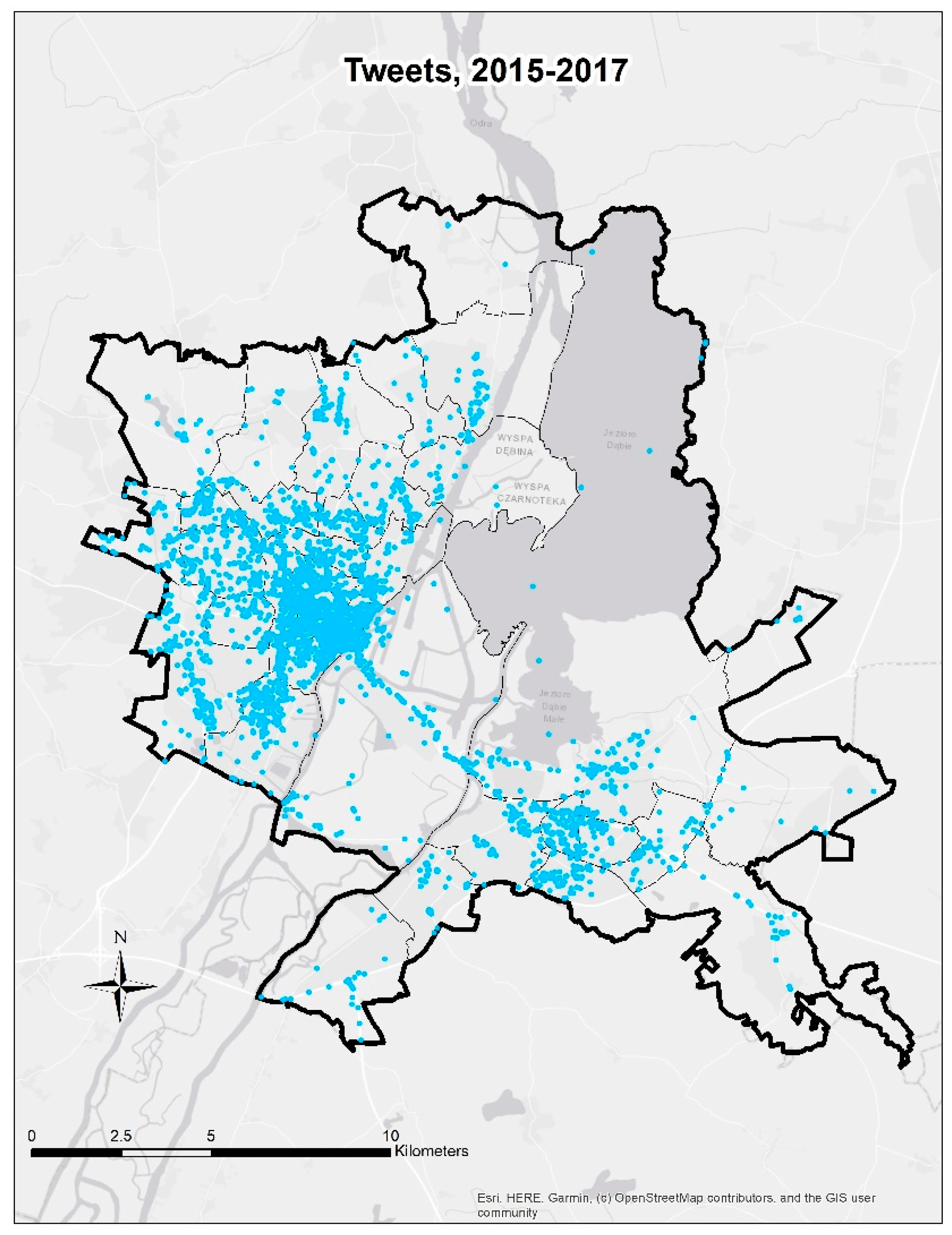
How can one estimate the size of the ambient population in individual neighborhoods of a large city?
(2)
What is the relationship between the size of the ambient population (Group 1) and different types of crime, with socioeconomic characteristics controlled?
(3)
What is the relationship between the size of the immobile population (Group 2) and different types of crime, with socioeconomic characteristics controlled?
These questions reflect the level of originality and the novelty of the approach used in this study. It is crucial to distinguish between two groups of the population, with varying degrees of risk of crime: mobile and immobile. This was done using two different estimation methods: the number of tweeds posted in a given neighborhood, which is rarely used in the region. On this basis, the ambient population was estimated. Another innovation is taking into account not only ambient and immobile population relations in the research, but also socioeconomic characteristics that are important for crime opportunities. It is also worth emphasizing the significant number of crime types being analyzed.

3. Data and Methodology

We collected 3-year crime data in Szczecin, Poland (2015–2017), including (1) burglary in commercial buildings, (2) drug crime, (3) fight and battery, (4) property damage, and (5) theft. Following established practices in the field, we combined 3 years of data to overcome the limitation of the small number of incidents in each year [51,52,53,54]. This is acceptable due to the spatial distribution of crime in a city being stable over years [5,53,55]. Szczecin is the capital of the West Pomeranian Voivodeship in northwestern Poland. It is a major seaport as it is near the Baltic Sea and the German border. In 2015, it had a population of 404,712, and this number slightly declined to 404,000 in 2017. The size of the city is 301 km2, and it is composed of 37 neighborhoods. The city lies on the delta of the Oder River and is known as the “Paris of the North”, because of the characteristic star-shaped layout of streets and squares [56].
Burglaries in commercial buildings (2228) are distributed throughout the inhabited area of the city (Figure 1). They are mostly concentrated in the downtown area (the central-western area just west of the Oder River), which results from the fact that there are many, usually small, commercial and busy facilities in this area. They are usually located on the ground floors of mix-used buildings and in small pavilions which are typically easy to break into because of the lack of security measures. Large commercial and service centers, of which there are about ten in Szczecin, are well guarded by closed-circuit television (CCTV) and security measures, so they are not frequent targets of commercial burglaries. Such information comes from local law enforcement officers and scholars.
Drug crime incidents (2060) occur throughout the entire inhabited area of the city but are clearly concentrated in the central part of downtown and an area north of it known for its high overall crime rate (Figure 2).
Fights and batteries (1709) have a similar spatial distribution. A high concentration occurs in the central part of downtown. This is related to the fact that there is a significant concentration of alcohol distribution points in this area (catering outlets, alcohol shops, grocery stores, etc.). As local residents and law enforcement officers indicate, alcohol consumption strongly influences this type of crime. Apart from that, the downtown area has a sizable number of people who are known to be bad-tempered (Figure 3).
Property damages (1844) have a similar distribution too, which results from the conditions of the population described above. The concentration of this crime type in the downtown area is even more obvious (Figure 4).
The most common type of crime–theft (10,100)—is almost everywhere across the entire inhabited areas of the city, and the concentration of these crime incidents in the downtown area is not as dominant. This is due to the fact that the victims of the theft are individuals, and they can be mobile (Figure 5).
We collected tweets from 2015 to 2017 in the same city through TweetScraper, a Python script built on Scrapy without using Twitter’s APIs [57]. Scrapy is an open-source and collaborative framework for extracting data from websites [58]. According to the tool description, TweetScraper mimics the Tweet Search on a web browser and can bypass the Twitter API’s 1% limit, enabling it to crawl all publicly available tweets. Clearly, the spatial distribution of tweets (Figure 6) is remarkably similar to the aforementioned crime types, especially thefts (Figure 5).
We use the neighborhood of the city as the unit of analysis, and there are 37 neighborhoods in total. The neighborhood is the finest unit of sociodemographic data which is available in this city. Therefore, though we can collect point-level crime data and tweets, we have to aggregate them to the neighborhood level to compare them with age structure and other sociodemographic factors. The dependent variables are the counts of each crime type. The independent variables are twofold: (1) tweet count as an ambient population measure [11,12,14,31,43], and (2) young (≤15) and elderly (>65) population as a measure of people with limited mobility, hereafter referred to as the immobile population [59]. The control socioeconomic variables are population density, population assisted by the Municipal Family Assistance Center, unemployed population, demographic load index (an age-structure indicator calculating the percentage of non-productive age population), and count of liquor stores in 2015 [52,60,61,62,63,64,65].
Table 1 shows descriptive statistics of variables. Five dependent variables are counts of burglary in commercial buildings (commercial burglaries), drug crime, fight and battery (assault), property damage (vandalism), and theft. Two major independent variables are the tweets-derived ambient population and the immobile population (population under age 16 or older than 65). Additional control variables are population density (a measure of population concentration), population assisted by the municipal family assistance center (people in poverty), unemployed population (people who are not employed), demographic load index (shows the burden to the society by the unproductive population), and the count of liquor stores (known to be related to many violent and property crime types) [52,60,61,62,63,64,65]. The control variables in this study are additional independent variables that are not of direct interest to this study’s goals but are controlled because they have been tested by previous studies to influence crime patterns. We include them to make sure the crime–tweets relationship and the crime–age structure relationship are not accidental. For each of these five dependent variables, two models are fit, one with the ambient population (tweets) and controls, another with the immobile population (≤15 or >65) and controls. Consequently, 2 × 5 = 10 models are fit.
To use a traditional linear regression model, the dependent variable needs to follow the normal distribution. However, as Law of Crime Concentration and Iron Law of Troublesome Places suggest: few places are responsible for most of the crime, and most places do not experience any crime, so the distribution of crime is always skewed [5,6,8,9]. As evidenced in Figure 1, Figure 2, Figure 3, Figure 4 and Figure 5, crime patterns in Szczecin are also clustered. This clearly violates the basic assumption of linear regression; thus, Poisson or negative binomial regression should be used [66,67,68]. The Poisson regression model may be used for count data like crime incidents. However, to use Poisson regression, the dependent variable’s mean needs to be equal to the variance, which is often not satisfied in crime data. Therefore, following the general practice in crime studies, we use the negative binomial regression model to assess the relationship between crime and the ambient population versus the immobile population (≤15 and >65). The negative binomial regression model has been widely used in criminology studies because it does not assume homogeneity of variance and does not require normal distribution of the dependent variable [67]. The unit of analysis is the neighborhood (N = 37). The negative binomial regression model is:
y i   ~   N B [ e x p ( β k x i k ) , α ]
where NB stands for negative binominal, y i is the crime count in the ith (i = 1, …, n) neighborhood, x i k is the kth explanatory variable for neighborhood i, β k (k = 0, 1, …, p) are the coefficients, and α is the parameter of overdispersion [68].

4. Results and Discussion

Table 2 shows the results of negative binomial models for five different crime types. As specified in the methodology section, each of these five crime types is fit with two different models: one with the ambient population (tweets), and one with the immobile population (≤15 or >65). All models also contain necessary control socioeconomic variables, and the sample size of each model is 37. The tweet-based ambient population measure has a positively significant relationship with all five crime types: commercial burglary (β = 0.53, p < 0.05), drug crime (β = 0.44, p < 0.01), fight-battery (β = 0.34, p < 0.01), property damage (β = 0.36, p < 0.05), and theft (β = 0.09, p < 0.01). This means that if the neighborhood has more ambient population, the risks of these crimes tend to be higher. These five types of crime are all closely related to the dynamic distribution of population on and near streets: commercial burglary happens in commercial facilities and commercial facilities where people frequent [69]; drug crime (including distributing, dispensing, possessing, dealing drugs), fight-battery, property damage (vandalism), and thefts tend to happen on streets and near streets where people visit [12,70,71,72,73].
The immobile population (≤15 or >65), however, is only significantly related to commercial burglaries in a positive manner. A probable reason for this is in Szczecin, residential and commercial structures are highly mixed, and neighborhoods have more residential dwellings and commercial facilities. In addition, the less mobile populations tend to use only shops and service establishments close to their place of residence. Coincidently, offenders of commercial burglaries are also mainly residents of a given area, and they tend to target small premises that are poorly protected [74,75].
Regarding the control variables, population density is negatively related to commercial burglaries in Szczecin. This may suggest that areas with smaller population density experience more commercial burglaries. A potential explanation is that burglars tend to avoid super busy areas as the risk of being identified is higher because more people are nearby, and commercial facilities in those areas typically utilize more security measures to prevent burglaries [76,77]. Areas with more population in poverty and unemployed tend to experience more commercial burglaries, drug problems, property damage, and thefts as suggested in previous studies [70,78,79,80]. Additionally, the count of liquor stores is positively related to drug crime, fight-battery, and theft, which parallels well with existing literature [81,82,83].
It is necessary to acknowledge the limitations of social media data like tweets. As previous studies have discovered, tweets may not represent the whole picture of the census population in an area. This is because Twitter users are relatively young, urban residents, and mobile users [44,48,49]. Additionally, only 15% of internet-using adults use Twitter, and most of them are young adults [84,85]. Thus, analyses based on tweets should not overstate claims about the representativeness of the data. Nevertheless, these limitations do not undermine the discoveries of this study, as we use the tweet count as a measure for the population who are more mobile. Results suggest that the distribution of mobile and immobile populations is correlated with the patterns of different crime types. Due to data limitations, we are only able to conduct this study in Szczecin, Poland. More tests should be done in other European countries, or even other parts of the world in order to further improve the discipline and advance knowledge. Further, we use the neighborhood as the study unit because that is the finest unit of sociodemographic data we could obtain in this area. As suggested by a previous study, the study unit size may influence the results due to the modifiable areal unit problem (MAUP) [31]. Thus, if data are available, more tests may be needed at even finer spatial units, e.g., track, block group, and blocks, in order to see whether such relationships persist across different spatial scales.

5. Conclusions

The main goal of the article has been achieved. The adopted method of estimating the ambient population based on geotagged tweets turned out to be effective, justified, and providing of fruitful research, as suggested in various previous studies. The same applies to the estimation of the immobile population from age structure. Using both mobile and immobile social groups creates a new perspective for researching crime in cities. Utilizing negative binomial regression models, a positive correlation is found between the size of the ambient population and all investigated crime types (burglary in commercial buildings, drug crime, fight and battery, property damage, and theft). While the distribution of immobile social groups is only related to commercial burglaries. Areas with more population in poverty and unemployment tend to experience more commercial burglaries, drug problems, property damage, and thefts. Additionally, the count of liquor stores is positively related to drug crime, fight-battery, and theft. As found in this study, the residents’ age structure may influence crime patterns in the city. Thus, when analyzing and preventing crime, the dynamic distribution of people with different mobile abilities needs to be considered.
As discussed in the earlier section, more tests in other regions and at different spatial scales are recommended. Comparison studies among different cities across countries can also be beneficial using the same method. This procedure, commonly found in experimental sciences, is seldom used in the social sciences. However, it should be taken into account that in different socioeconomic conditions, the control variables may have different meanings and require different interpretations. The overall level of crime in a country or region is also relevant in such surveys. In Poland it is relatively low, in Szczecin it is average compared to the rest of the country, and the most serious crimes with the use of weapons and murders are practically isolated cases.
The assumption that age structure and mobile ability need to be systematically considered in crime analysis studies should also be verified in other cities, but with a similar population age structure, level, and lifestyle. In more affluent countries, young people and the elderly are generally more mobile thanks to individual and collective means of transportation.
In future studies, it should be checked as well whether the applied methods of estimating the number of mobile and immobile populations reflect their real mobility. Such an experimental study, using detailed lists of residents obtained, for example, from property owners and CCTV cameras, could verify the assumptions of this method and indicate the level of possible error.

Author Contributions

Conceptualization, Natalia Sypion-Dutkowska and Marek Dutkowski; methodology, Minxuan Lan; software, Minxuan Lan; validation, Natalia Sypion-Dutkowska and Minxuan Lan; formal analysis, Minxuan Lan; investigation, Minxuan Lan; resources, Natalia Sypion-Dutkowska; data curation, Natalia Sypion-Dutkowska; writing—original draft preparation, Natalia Sypion-Dutkowska, Minxuan Lan and Marek Dutkowski; writing—review and editing, Minxuan Lan and Victoria Williams; visualization, Minxuan Lan; supervision, Natalia Sypion-Dutkowska and Minxuan Lan; project administration, Natalia Sypion-Dutkowska; funding acquisition, Natalia Sypion-Dutkowska All authors have read and agreed to the published version of the manuscript.

Funding

The project is financed by the National Science Centre, Poland, UMO-2019/35/D/HS4/02942.

Conflicts of Interest

The authors declare no conflict of interest.

References

  1. Brantingham, P.L.; Brantingham, P.J. Crime pattern theory. In Environmental Criminology and Crime Analysis; Wortley, R., Mazerolle, L., Eds.; Willan: Devon, UK, 2008; pp. 78–93. [Google Scholar] [CrossRef]
  2. Cohen, L.E.; Felson, M. Social Change and Crime Rate Trends: A Routine Activity Approach. Am. Sociol. Rev. 1979, 44, 588–608. [Google Scholar] [CrossRef]
  3. Al Baghal, T.; Sloan, L.; Jessop, C.; Williams, M.L.; Burnap, P. Linking Twitter and survey data: The impact of survey mode and demographics on consent rates across three UK studies. Soc. Sci. Comput. Rev. 2020, 38, 517–532. [Google Scholar] [CrossRef] [Green Version]
  4. Kinney, J.B.; Brantingham, P.L.; Wuschke, K.; Kirk, M.G.; Brantingham, P.J. Crime attractors, generators and detractors: Land use and urban crime opportunities. Built Environ. 2008, 34, 62–74. [Google Scholar] [CrossRef]
  5. Weisburd, D. The law of crime concentration and the criminology of place. Criminology 2015, 53, 133–157. [Google Scholar] [CrossRef]
  6. Wilcox, P.; Eck, J.E. Criminology of the unpopular: Implications for policy aimed at payday lending facilities. Criminol. Public Policy 2011, 10, 473–482. [Google Scholar] [CrossRef]
  7. Sypion-Dutkowska, N.; Leitner, M.; Dutkowski, M.J.C. Impact of metropolization on the crime structure (case study of provincial capitals in Poland). Cities 2021, 119, 103359. [Google Scholar] [CrossRef]
  8. Sherman, L.W.; Gartin, P.R.; Buerger, M.E. Hot spots of predatory crime: Routine activities and the criminology of place. Criminology 1989, 27, 27–56. [Google Scholar] [CrossRef]
  9. Weisburd, D.; Eck, J.E.; Braga, A.A.; Telep, C.W.; Cave, B.; Bowers, K.; Bruinsma, G.; Gill, C.; Groff, E.; Hibdon, J.; et al. Place Matters; Cambridge University Press: Cambridge, UK, 2016. [Google Scholar] [CrossRef]
  10. Andresen, M.A.; Malleson, N. Crime seasonality and its variations across space. Appl. Geogr. 2013, 43, 25–35. [Google Scholar] [CrossRef]
  11. Hipp, J.R.; Bates, C.; Lichman, M.; Smyth, P. Using Social Media to Measure Temporal Ambient Population: Does it Help Explain Local Crime Rates? Justice Q. 2019, 36, 718–748. [Google Scholar] [CrossRef] [Green Version]
  12. Lan, M.; Liu, L.; Hernandez, A.; Liu, W.; Zhou, H.; Wang, Z. The Spillover Effect of Geotagged Tweets as a Measure of Ambient Population for Theft Crime. Sustainability 2019, 11, 6748. [Google Scholar] [CrossRef] [Green Version]
  13. Ristea, A.; Andresen, M.A.; Leitner, M. Using tweets to understand changes in the spatial crime distribution for hockey events in Vancouver. Can. Geogr. 2018, 62, 338–351. [Google Scholar] [CrossRef] [Green Version]
  14. Williams, M.L.; Burnap, P.; Sloan, L. Crime Sensing with Big Data: The Affordances and Limitations of using Open Source Communications to Estimate Crime Patterns. Br. J. Criminol. 2016, 57, 320–340. [Google Scholar] [CrossRef] [Green Version]
  15. He, L.; Páez, A.; Jiao, J.; An, P.; Lu, C.; Mao, W.; Long, D. Ambient population and larceny-theft: A spatial analysis using mobile phone data. ISPRS Int. J. Geo-Inf. 2020, 9, 342. [Google Scholar] [CrossRef]
  16. McPherson, T.N.; Brown, M.J. Estimating Daytime and Nighttime Population Distributions in US Cities for Emergency Response Activities; Los Alamos National Laboratory (LANL): Los Alamos, NM, USA, 2003. [Google Scholar]
  17. Andresen, M.A. Crime measures and the spatial analysis of criminal activity. Br. J. Criminol. 2005, 46, 258–285. [Google Scholar] [CrossRef]
  18. Andresen, M.A.; Jenion, G.W. Ambient populations and the calculation of crime rates and risk. Secur. J. 2010, 23, 114–133. [Google Scholar] [CrossRef]
  19. Patel, N.N.; Stevens, F.R.; Huang, Z.; Gaughan, A.E.; Elyazar, I.; Tatem, A.J. Improving Large Area Population Mapping Using Geotweet Densities. Trans. GIS 2017, 21, 317–331. [Google Scholar] [CrossRef] [PubMed]
  20. Blank, G. The digital divide among Twitter users and its implications for social research. Soc. Sci. Comput. Rev. 2017, 35, 679–697. [Google Scholar] [CrossRef]
  21. Gong, X.; Wang, Y. Exploring dynamics of sports fan behavior using social media big data-A case study of the 2019 National Basketball Association Finals. Appl. Geogr. 2021, 129, 102438. [Google Scholar] [CrossRef]
  22. Yan, Y.; Chen, J.; Wang, Z. Mining public sentiments and perspectives from geotagged social media data for appraising the post-earthquake recovery of tourism destinations. Appl. Geogr. 2020, 123, 102306. [Google Scholar] [CrossRef]
  23. Sloan, L.; Morgan, J.; Burnap, P.; Williams, M. Who tweets? Deriving the demographic characteristics of age, occupation and social class from twitter user meta-data. PLoS ONE 2015, 10, e0115545. [Google Scholar] [CrossRef] [Green Version]
  24. Andrienko, G.; Andrienko, N.; Bosch, H.; Ertl, T.; Fuchs, G.; Jankowski, P.; Thom, D. Thematic Patterns in Georeferenced Tweets through Space-Time Visual Analytics. Comput. Sci. Eng. 2013, 15, 72–82. [Google Scholar] [CrossRef]
  25. Gerber, M.S. Predicting crime using Twitter and kernel density estimation. Decis. Support Syst. 2014, 61, 115–125. [Google Scholar] [CrossRef]
  26. Santhiya, K.; Bhuvaneswari, V.; Murugesh, V. Automated Crime Tweets Classification and Geo-location Prediction using Big Data Framework. Turk. J. Comput. Math. Educ. (TURCOMAT) 2021, 12, 2133–2152. [Google Scholar]
  27. Vomfell, L.; Härdle, W.K.; Lessmann, S. Improving crime count forecasts using Twitter and taxi data. Decis. Support Syst. 2018, 113, 73–85. [Google Scholar] [CrossRef]
  28. Andresen, M.A. The ambient population and crime analysis. Prof. Geogr. 2011, 63, 193–212. [Google Scholar] [CrossRef]
  29. Malleson, N.; Andresen, M.A. Spatio-temporal crime hotspots and the ambient population. Crime Sci. 2015, 4, 10. [Google Scholar] [CrossRef] [Green Version]
  30. Wang, Z.; Li, Y. Could social medias reflect acquisitive crime patterns in London? J. Saf. Sci. Resil. 2022, 3, 115–127. [Google Scholar] [CrossRef]
  31. Liu, L.; Lan, M.; Eck, J.E.; Yang, B.; Zhou, H. Assessing the Intraday Variation of the Spillover Effect of Tweets-Derived Ambient Population on Crime. Soc. Sci. Comput. Rev. 2020, 40, 512–533. [Google Scholar] [CrossRef]
  32. Lal, S.; Tiwari, L.; Ranjan, R.; Verma, A.; Sardana, N.; Mourya, R. Analysis and classification of crime tweets. Procedia Comput. Sci. 2020, 167, 1911–1919. [Google Scholar] [CrossRef]
  33. Roitman, H.; Mamou, J.; Mehta, S.; Satt, A.; Subramaniam, L. Harnessing the crowds for smart city sensing. In Proceedings of the 1st International Workshop on Multimodal Crowd Sensing, Maui, HI, USA, 2 November 2012; pp. 17–18. [Google Scholar]
  34. Lampoltshammer, T.J.; Kounadi, O.; Sitko, I.; Hawelka, B. Sensing the public’s reaction to crime news using the ‘Links Correspondence Method’. Appl. Geogr. 2014, 52, 57–66. [Google Scholar] [CrossRef]
  35. Bendler, J.; Ratku, A.; Neumann, D. Crime mapping through geo-spatial social media activity. In Proceedings of the Thirty Fifth International Conference on Information Systems, Auckland, New Zealand, 14–17 December 2014. [Google Scholar]
  36. Bendler, J.; Brandt, T.; Wagner, S.; Neumann, D. Investigating crime-to-twitter relationships in urban environments-facilitating a virtual neighborhood watch. In Proceedings of the European Conference on Information Systems (ECIS) 2014, Tel Aviv, Israel, 9–11 June 2014. [Google Scholar]
  37. Liew, S.W.; Sani, N.F.M.; Abdullah, M.T.; Yaakob, R.; Sharum, M.Y. An effective security alert mechanism for real-time phishing tweet detection on Twitter. Comput. Secur. 2019, 83, 201–207. [Google Scholar] [CrossRef]
  38. Ristea, A.; Al Boni, M.; Resch, B.; Gerber, M.S.; Leitner, M. Spatial crime distribution and prediction for sporting events using social media. Int. J. Geogr. Inf. Sci. 2020, 34, 1708–1739. [Google Scholar] [CrossRef] [PubMed] [Green Version]
  39. Müller, K.; Schwarz, C. From Hashtag to Hate Crime: Twitter and Anti-Minority Sentiment. 2020. Available online: https://ssrn.com/abstract=3149103 (accessed on 1 May 2022).
  40. Nguyen, T.T.; Huang, D.; Michaels, E.K.; Glymour, M.M.; Allen, A.M.; Nguyen, Q.C. Evaluating associations between area-level Twitter-expressed negative racial sentiment, hate crimes, and residents’ racial prejudice in the United States. SSM-Popul. Health 2021, 13, 100750. [Google Scholar] [CrossRef] [PubMed]
  41. Sharma, N.; Dhamne, A.; More, N.; Rathi, V.; Supekar, A. Detection of crime and non-crime tweets using Twitter. Int. J. Adv. Res. Comput. Commun. Eng. 2018, 7, 229–232. [Google Scholar]
  42. Ristea, A.; Langford, C.; Leitner, M. Relationships between crime and Twitter activity around stadiums. In Proceedings of the 2017 25th International Conference on Geoinformatics, Buffalo, NY, USA, 2–4 August 2017; pp. 1–5. [Google Scholar]
  43. Lan, M.; Liu, L.; Burmeister, J.; Zhu, W.; Zhou, H.; Gu, X. Are Crime and Collective Emotion Interrelated? A “Broken Emotion” Conjecture from Community Twitter Posts. Soc. Sci. Comput. Rev. 2022, 1–26. [Google Scholar] [CrossRef]
  44. Duggan, M.; Brenner, J. The Demographics of Social Media Users, 2012; Pew Research Center’s Internet & American Life Project: Washington, DC, USA, 2013; Volume 14. [Google Scholar]
  45. Malik, M.M.; Lamba, H.; Nakos, C.; Pfeffer, J. Population bias in geotagged tweets. In Proceedings of the Ninth International AAAI Conference on Web and Social Media, Oxford, UK, 26–29 May 2015. [Google Scholar]
  46. IPSOS Media CT Tech Tracker—Quarterly Release: Q3 2014. 2014. Available online: https://www.yumpu.com/en/document/read/34392898/ipsosmediact-techtracker-q3-2014 (accessed on 1 May 2022).
  47. Zou, L.; Lam, N.S.; Cai, H.; Qiang, Y. Mining Twitter data for improved understanding of disaster resilience. Ann. Am. Assoc. Geogr. 2018, 108, 1422–1441. [Google Scholar] [CrossRef]
  48. Gleason, B. Thinking in hashtags: Exploring teenagers’ new literacies practices on Twitter. Learn. Media Technol. 2018, 43, 165–180. [Google Scholar] [CrossRef] [Green Version]
  49. Cao, X.; MacNaughton, P.; Deng, Z.; Yin, J.; Zhang, X.; Allen, J. Using twitter to better understand the spatiotemporal patterns of public sentiment: A case study in Massachusetts, USA. Int. J. Environ. Res. Public Health 2018, 15, 250. [Google Scholar] [CrossRef] [Green Version]
  50. Hamstead, Z.A.; Fisher, D.; Ilieva, R.T.; Wood, S.A.; McPhearson, T.; Kremer, P. Geolocated social media as a rapid indicator of park visitation and equitable park access. Comput. Environ. Urban Syst. 2018, 72, 38–50. [Google Scholar] [CrossRef]
  51. Bernasco, W.; Block, R. Robberies in Chicago: A block-level analysis of the influence of crime generators, crime attractors, and offender anchor points. J. Res. Crime Delinq. 2011, 48, 33–57. [Google Scholar] [CrossRef] [Green Version]
  52. Haberman, C.P.; Ratcliffe, J.H. Testing for temporally differentiated relationships among potentially criminogenic places and census block street robbery counts. Criminology 2015, 53, 457–483. [Google Scholar] [CrossRef]
  53. Haberman, C.P.; Sorg, E.T.; Ratcliffe, J.H. The Seasons They Are a Changin’ Testing for Seasonal Effects of Potentially Criminogenic Places on Street Robbery. J. Res. Crime Delinq. 2018, 55, 425–459. [Google Scholar] [CrossRef]
  54. Liu, L.; Zhou, H.; Lan, M. Agglomerative Effects of Crime Attractors and Generators on Street Robbery? An Assessment by Luojia 1-01 Satellite Nightlight. Ann. Am. Assoc. Geogr. 2022, 112, 350–367. [Google Scholar] [CrossRef]
  55. Liu, L.; Lan, M.; Eck, J.E.; Kang, E.L. Assessing the effects of bus stop relocation on street robbery. Comput. Environ. Urban Syst. 2020, 80, 101455. [Google Scholar] [CrossRef]
  56. Banaszek, A. SZCZECIN. The City of Many faces. Kraków Airport Blog. 2016. Available online: https://krakowairport.pl/blog/en/szczecin-miasto-o-wielu-obliczach/ (accessed on 1 May 2022).
  57. Bakerfish, J. TweetScraper. Available online: https://github.com/jonbakerfish/TweetScraper (accessed on 1 May 2022).
  58. Zyte. Scrapy. Available online: https://scrapy.org/ (accessed on 1 May 2022).
  59. Krisjane, Z.; Apsite-Berina, E.; Berzins, M.; Grine, I. Regional topicalities in Latvia: Mobility and immobility in the countryside. In Proceedings of the Economic Science for Rural Development, Jelgava, Latvia, 27–28 April 2017. [Google Scholar]
  60. Parker, R.N.; Auerhahn, K. Alcohol, drugs, and violence. Annu. Rev. Sociol. 1998, 24, 291–311. [Google Scholar] [CrossRef]
  61. Lan, M.; Liu, L.; Eck, J.E. A spatial analytical approach to assess the impact of a casino on crime: An example of JACK Casino in downtown Cincinnati. Cities 2021, 111, 103003. [Google Scholar] [CrossRef]
  62. Harries, K. Property crimes and violence in United States: An analysis of the influence of population density. Int. J. Crim. Justice Sci. 2006, 1. [Google Scholar]
  63. Wolniak, R. Social Welfare Organisation in Poland. In Scientific Papers of Silesian University of Technology Organization and Management Series; No. 143; Silesian University of Technology: Gliwice, Poland, 2020. [Google Scholar]
  64. Majka, A.; Zając, D. Factors Influencing the Development of Non-Agricultural Business Activities in Rural Eastern Poland. Acta Sci. Polonorum. Oeconomia 2019, 18, 43–52. [Google Scholar] [CrossRef]
  65. Grshybowskyj, J.L.; Smiianov, V.A.; Myronyuk, I.M.; Lyubinets, O.V. Ten Indicators Which Characterize Medical-Demographic Processes in Adjacent Regions of Ukraine and Poland. Wiad. Lek. 2019, 72, 868–876. [Google Scholar] [CrossRef]
  66. Nagin, D.S.; Land, K.C. Age, criminal careers, and population heterogeneity: Specification and estimation of a nonparametric, mixed Poisson model. Criminology 1993, 31, 327–362. [Google Scholar] [CrossRef]
  67. Osgood, D.W. Poisson-based regression analysis of aggregate crime rates. J. Quant. Criminol. 2000, 16, 21–43. [Google Scholar] [CrossRef]
  68. Chen, J.; Liu, L.; Xiao, L.; Xu, C.; Long, D. Integrative analysis of spatial heterogeneity and overdispersion of crime with a geographically weighted negative binomial model. ISPRS Int. J. Geo-Inf. 2020, 9, 60. [Google Scholar] [CrossRef] [Green Version]
  69. Butler, G. Commercial burglary: What offenders say. In Crime at Work; Springer: Berlin/Heidelberg, Germany, 2005; pp. 29–41. [Google Scholar]
  70. Zhou, H.; Liu, L.; Lan, M.; Zhu, W.; Song, G.; Jing, F.; Zhong, Y.; Su, Z.; Gu, X. Using Google Street View imagery to capture micro built environment characteristics in drug places, compared with street robbery. Comput. Environ. Urban Syst. 2021, 88, 101631. [Google Scholar] [CrossRef]
  71. Weeks, M.R.; Grier, M.; Romero-Daza, N.; Puglisi-Vasquez, M.J.; Singer, M. Streets, drugs, and the economy of sex in the age of AIDS. Women Health 1998, 27, 205–229. [Google Scholar] [CrossRef]
  72. Taylor, D.; Eddey, D.; Cameron, P. Demography of assault in a provincial Victorian population. Aust. N. Z. J. Public Health 1997, 21, 53–58. [Google Scholar] [CrossRef] [PubMed]
  73. Poyner, B. Design against Crime: Beyond Defensible Space; Butterworths London: London, UK, 1983. [Google Scholar]
  74. Bernasco, W.; Kooistra, T. Effects of residential history on commercial robbers’ crime location choices. Eur. J. Criminol. 2010, 7, 251–265. [Google Scholar] [CrossRef] [Green Version]
  75. Sohn, D.-W. Do all commercial land uses deteriorate neighborhood safety?: Examining the relationship between commercial land-use mix and residential burglary. Habitat Int. 2016, 55, 148–158. [Google Scholar] [CrossRef]
  76. Schmalleger, F. Criminology, 5th ed.; Pearson: Upper Saddle River, NJ, USA, 2018. [Google Scholar]
  77. Tseloni, A.; Thompson, R.; Grove, L.; Tilley, N.; Farrell, G. The effectiveness of burglary security devices. Secur. J. 2017, 30, 646–664. [Google Scholar] [CrossRef] [Green Version]
  78. Zhou, H.; Liu, L.; Lan, M.; Yang, B.; Wang, Z. Assessing the Impact of Nightlight Gradients on Street Robbery and Burglary in Cincinnati of Ohio State, USA. Remote Sens. 2019, 11, 1958. [Google Scholar] [CrossRef] [Green Version]
  79. Valdez, A.; Kaplan, C.D.; Curtis, R.L., Jr. Aggressive crime, alcohol and drug use, and concentrated poverty in 24 US urban areas. Am. J. Drug Alcohol Abus. 2007, 33, 595–603. [Google Scholar] [CrossRef]
  80. Unnever, J.D. Direct and organizational discrimination in the sentencing of drug offenders. Soc. Probl. 1982, 30, 212–225. [Google Scholar] [CrossRef]
  81. Gruenewald, P.J.; Freisthler, B.; Remer, L.; LaScala, E.A.; Treno, A. Ecological models of alcohol outlets and violent assaults: Crime potentials and geospatial analysis. Addiction 2006, 101, 666–677. [Google Scholar] [CrossRef] [PubMed]
  82. Gorman, D.M.; Speer, P.W.; Gruenewald, P.J.; Labouvie, E.W. Spatial dynamics of alcohol availability, neighborhood structure and violent crime. J. Stud. Alcohol 2001, 62, 628–636. [Google Scholar] [CrossRef] [PubMed]
  83. Zhu, L.; Gorman, D.M.; Horel, S. Alcohol outlet density and violence: A geospatial analysis. Alcohol Alcohol. 2004, 39, 369–375. [Google Scholar] [CrossRef] [PubMed] [Green Version]
  84. Widener, M.J.; Li, W. Using geolocated Twitter data to monitor the prevalence of healthy and unhealthy food references across the US. Appl. Geogr. 2014, 54, 189–197. [Google Scholar] [CrossRef]
  85. Smith, A.; Brenner, J. Twitter Use 2012; Pew Research Center’s Internet & American Life Project: Washington, DC, USA, 2012; Volume 4, pp. 1–12. [Google Scholar]
Figure 1. Burglaries in Commercial Buildings in Szczecin, 2015–2017 (n = 2228).
Ijgi 11 00581 g001
Figure 2. Drug crime in Szczecin, 2015–2017 (n = 2060).
Ijgi 11 00581 g002
Figure 3. Fights and batteries in Szczecin, 2015–2017 (n = 1709).
Ijgi 11 00581 g003
Figure 4. Property damages in Szczecin, 2015–2017 (n = 1844).
Ijgi 11 00581 g004
Figure 5. Thefts in Szczecin, 2015–2017 (n = 10,100).
Ijgi 11 00581 g005
Figure 6. Tweets in Szczecin, 2015–2017 (n = 26,719).
Ijgi 11 00581 g006
Table 1. Descriptive statistics.
Variables (2015–2017)MinimumMaximumMeanStd. Deviation
DependentBurglary in commercial buildings416160.2240.09
Drug crime134555.6874.03
Fight and battery331346.1957.74
Property damage420149.8446.33
Theft91369272.97268.86
IndependentAmbient population (Tweets)62322723.14688.43
Immobile population (≤15 or >65)29280943269.572328.62
ControlPopulation density3327,3894570.835831.37
Population assisted by the Municipal Family Assistance Center11950281.24250.35
Unemployed population511083312.78237.58
Demographic load index31.106645.108.82
Count of liquor stores327954.7052.77
Table 2. Results of negative binomial regression models.
Standardized Coefficient (* 10−2)
Burglary in Commercial BuildingsDrug CrimeFight and BatteryProperty DamageTheft
Model 1Model 2Model 3Model 4Model 5Model 6Model 7Model 8Model 9Model 10
Ambient population (Tweets)0.53 * 0.44 ** 0.34 ** 0.36 * 0.09 **
Immobile population with (≤15 or >65) 2.07 *** 1.07 1.13 1.56 0.37
Population density−0.29−0.5**0.210.10.02−0.080.29 *0.190.01−0.02
Population assisted by the Municipal Family Assistance Center−0.071.3*0.741.59 *0.561.40.081.16−0.020.24
Unemployed population1.75 ***−1.490.01−1.730.1−1.680.98 **−1.430.2 ***−0.37
Demographic load index0.34−0.160.23−0.010.18−0.060.26−0.020.02−0.05
Count of liquor stores−0.420.520.470.96 *0.91 *1.36 **0.510.980.130.26 *
Significance level: * < 0.05, ** < 0.01, *** < 0.001. Each models has a constant.
Publisher’s Note: MDPI stays neutral with regard to jurisdictional claims in published maps and institutional affiliations.

