Article

UAS Control under GNSS Degraded and Windy Conditions

by
Michail Kalaitzakis
and
Nikolaos Vitzilaios
*
Department of Mechanical Engineering, University of South Carolina, Columbia, SC 29208, USA
*
Author to whom correspondence should be addressed.
Robotics 2023, 12(5), 123; https://doi.org/10.3390/robotics12050123
Submission received: 28 July 2023 / Revised: 23 August 2023 / Accepted: 25 August 2023 / Published: 26 August 2023
(This article belongs to the Special Issue UAV Systems and Swarm Robotics)

Abstract

:
Multirotor Uncrewed Aircraft Systems (UAS), widely known as aerial drones, are increasingly used in various indoor and outdoor applications. For outdoor field deployments, the plethora of UAS rely on Global Navigation Satellite Systems (GNSS) for their localization. However, dense environments and large structures can obscure the signal, resulting in a GNSS-degraded environment. Moreover, outdoor operations depend on weather conditions, and UAS flights are significantly affected by strong winds and possibly stronger wind gusts. This work presents a nonlinear model predictive position controller that uses a disturbance observer to adapt to changing weather conditions and fiducial markers to augment the system’s localization. The developed framework can be easily configured for use in multiple different rigid multirotor platforms. The effectiveness of the proposed system is shown through rigorous experimental work in both the lab and the field. The experimental results demonstrate consistent performance, regardless of the environmental conditions and platform used.

1. Introduction

Uncrewed Aircraft Systems (UAS), widely known as aerial drones, are increasingly used in infrastructure inspection applications [1], among others. Recent surveys show the extensive use of drones in non-destructive inspections of industrial sites [2] and in facility condition monitoring [3]. A technical report from the Minnesota Department of Transportation [4] shows that the use of drones can improve the quality of bridge inspections. Moreover, the significant advantages of drone-based inspections compared to traditional manual inspections were presented in a recent comparative study [5].
In most cases, the inspections are performed by manual or semi-autonomous flights, and one of the key research challenges is to build fully autonomous systems with collision-avoidance capabilities [1]. One of the biggest challenges in this effort is to maintain an accurate state estimation and robust position control. These are significantly affected by two factors: (i) degraded Global Navigation Satellite System (GNSS) signals, and (ii) changing weather conditions (wind and wind gusts).
The vast majority of aerial drones used for infrastructure inspections are dependent on the use of GNSS. However, GNSS signals are susceptible to signal degradation [6] and blockage when, for example, drones fly close to large structures or below bridges [7]. Without a reliable GNSS signal, there is a rapid deterioration in the navigation system of the drone since there are no position measurement updates, and attitude measurements are not enough to keep the system from drifting. In this case, different sensors and methods can be used as reliable alternatives to localization and navigation [8,9], including visual-based [10] and LIDAR-based [11] methods.
Moreover, in outdoor applications, wind remains a major disturbance and makes control challenging [12]. Since the early days of multirotor platforms, there have been studies on how winds affect them as systems [13]. A novel state parameter control based on Euler angles was discussed in [14] with a dynamic feedback controller and a Lyapunov estimation of the wind parameters. To estimate the effect of external disturbances, a sliding-mode observer was introduced in [15]. A feedback linearization-based controller ran in parallel with the estimator. This controller design allowed for the minimal use of sensors to estimate the state of the vehicle. Finally, a switching model predictive controller with piecewise affine models for the linearized dynamics of a quadrotor was presented in [16]. The quadrotor was tested indoors without the use of GNSS, using an experimental setup for the wind gusts.
Our group has developed a UAS system to perform Digital Image Correlation (DIC) measurements in railroad bridges [17,18]. GNSS-degraded signals and wind disturbances have been issues that we had to resolve toward building a fully autonomous system. Motivated by this goal, we developed and present in this paper a control framework for UAS field deployments close to large structures. The proposed system uses the UAS flight dynamics and a disturbance observer to estimate the external forces acting on the platform and a nonlinear model predictive controller that considers the platform dynamics and external forces to control the position of the platform.
To allow this framework to be used by multiple different rigid body multirotor UAS, a generic multirotor model is used. Furthermore, the framework is designed to work with PX4 Autopilot [19] Flight Control Units (FCU), one of the most widely used flight controllers. Finally, the different portions of the updated control framework are developed as ROS nodes [20], and the complete framework, as well as scripts that implement the required system identification, are made publicly available at https://github.com/usrl-uofsc/px4_control (accessed on 20 July 2023).
The effectiveness of the proposed system is shown through a series of lab tests using a Motion Capture (MoCap) system. The framework’s ability to estimate the external forces acting on the platform, augment its localization using pose information from fiducial markers, and ultimately track the desired trajectory under changing wind conditions is examined. Finally, the proposed system is deployed in a second, different, and larger UAS, performing a bridge inspection. Experimental results in both cases show consistent performance for both multirotor UAS.
In summary, the main contributions of this work are (i) the development of a control framework for navigation in GNSS-degraded and windy environments that can be applied in any rigid multirotor platform; (ii) a rigorous experimental analysis that includes both indoor and outdoor flights with two different platforms, demonstrating the effectiveness of the framework; and (iii) the developed framework is made publicly available to the community.
The rest of the paper is organized as follows. Section 2 defines the system modeling, state estimation, and control portions of the proposed framework. Section 3 presents the experimental setup used to validate the effectiveness of the system and discusses the experimental findings. Finally, Section 4 concludes this work and discusses areas of interest that may be explored in the future.

2. System Modeling and Control

There has been a significant body of work in modeling external forces acting on UAS without using any extra sensors [21,22,23]. Most notable is the work from Tomić et al. [24,25]. The authors used the UAS dynamics model, along with models for the propeller and motor dynamics, to estimate the external forces and torques acting on the platform. Moreover, they were able to distinguish between aerodynamic, contact, and collision forces, even when they were applied in tandem. Although this system can be used to accurately estimate all external disturbances, accurate models for all the components are needed. To obtain such models, a laborious system identification process is required.
Since one of the objectives of this work is to provide a framework that can quickly be deployed on multiple different platforms, only a simplified model for the rigid body dynamics is used. Moreover, the model does not consider the full wrench applied to the platform; only forces are considered. While this limits the accuracy of the estimated disturbances, it considerably simplifies the system identification process. Using data from a single manual flight, the parameters of the required model can be derived using classic system identification methods [26]. This is also significant during the development of a UAS when the design might change multiple times.

2.1. System Modeling

A nonlinear model of the UAS is required by both the state estimator and the controller. To define the six-degree-of-freedom (DoF) pose of the UAS, a fixed inertial frame (E) and a body frame (B), attached to the platform, need to be defined. Figure 1 shows a schematic of a hexrotor UAS with the body and inertial frames. While a hexrotor model is shown in the figure, the derived model for the dynamics can be used for multiple types of rigid body multirotors. The nonlinear model used for the UAS is:
p ˙ = v , v ˙ = d x 0 0 0 d y 0 0 0 d z v + R ( q ) 0 0 T 0 0 g + F e x t e r n a l , q ˙ = 1 2 q ω ,
where p E is the vector of the position of the origin of B, and v E is the linear velocity of B. The rotation matrix of B with respect to E is denoted by R; d x , d y , and d z are the mass-normalized drag coefficients; T is the mass-normalized thrust; g is the gravitational acceleration; and F e x t e r n a l is the mass-normalized external disturbances. The mass-normalized thrust is modeled as T = k T T c m d , where k T is the thrust coefficient and T c m d [ 0 , 1 ] is the thrust command. Finally, q is the rotation quaternion equivalent of the rotation matrix R, ⊗ denotes the quaternion product, and ω B is the angular velocity of B with respect to E, written as a pure quaternion.
While quaternions are used for the state estimation, the pitch ( ϕ ), roll ( θ ), and yaw ( ψ ) angles are used for the controller. Furthermore, it is assumed that a low-level attitude controller can track the desired roll and pitch angles ( ϕ d and θ d , respectively). A first-order model is used to model the response of the attitude controller for the roll and pitch. As for the yaw angle, it is assumed that the attitude controller can directly track the desired yaw rate ψ d ˙ . Finally,
ϕ ˙ = 1 τ ϕ ( k ϕ · ϕ d ϕ ) , θ ˙ = 1 τ θ ( k θ · θ d θ ) , ψ ˙ = ψ d ˙ ,
where τ ϕ and τ θ represent the time constants, and k ϕ and k θ represent the gain. Finally, the inputs to the system are T c m d , ϕ d , θ d , and ψ d ˙ .
To improve the position estimation in GNSS-degraded environments and mark areas of interest, fiducial markers can be used. As shown in Figure 1, the markers define a coordinate frame M. The frame M is assumed to be stationary with respect to the fixed frame E. As such, its position and attitude are modeled as:
p ˙ M = 0 , R ˙ M = 0 ,
where p M E is the vector of the position of the origin of M, and R M denotes the rotation matrix of M with respect to E.
It should be noted that this approach works for any orientation of the fiducial marker, as long as it is visible from the camera. In Figure 1, the marker is attached to a vertical surface but we can achieve similar performance when the marker is attached to a horizontal surface, in particular, to the underside of a structure [27].

2.2. State Estimation

The state and disturbance estimator is based on an Error State Kalman Filter (ESKF). The structure and derivation of the filter are based on [28]. There are three state values considered in the ESKF formulation: the true state χ t r u e , the nominal state χ , and the error state δ χ . The true state is the composition of the nominal and error states χ t r u e = χ δ χ . The nominal state should be considered the “large” part of the true state and can be calculated by integrating the nonlinear model of the system. The error state, however, should be considered the “small” part of the true state that accumulates all modeling errors and process noise. The ESKF estimates the error state instead of the true state and uses it to correct the nominal state.
The ESKF process is as follows. Using the inputs to the system and the model derived in Section 2.1, the state of the system is tracked by integrating the nonlinear system. However, the modeling errors and unmodeled dynamics will gradually accumulate in the error state, so the filter is propagated to predict a Gaussian estimate of the error state. When a measurement becomes available, the error state becomes observable and a filter correction is performed. The error state mean can then be calculated and injected into the nominal state.
There are a few advantages of using an ESKF compared to other Kalman Filters [28,29]. Compared to the EKF, the error state system operates closer to the origin, and thus the linearization assumption is more likely to hold. Also, the error state is small, and thus all higher-order products are indeed negligible, simplifying the computation of Jacobians. Since the generalized composition is used to correct the nominal state and find the true state, it simplifies working with constrained quantities such as rotations in 3D. Finally, it has been shown that the ESKF formulation performs better for mobile robot localization than the EKF formulation [30].
The three state values considered in the filter are shown in Table 1. The angles vector contains the error state of the UAS attitude quaternion. It is assumed that the GNSS position measurement contains both White and Brownian noise. To track the random bias of the Brownian noise, an extra state b t r u e is added to the filter.
To derive the dynamics of the true state, it is assumed that the modeling errors are additive and directly affect the velocity and attitude of the UAS:
p ˙ D t r u e = v D t r u e , v ˙ D t r u e = D v D t r u e + R T g + F t r u e + v m e , q ˙ D t r u e = 1 2 q D t r u e ( ω + ω m e ) , F ˙ t r u e = 0 , b ˙ t r u e = υ , p ˙ M t r u e = 0 , q ˙ M t r u e = 0 ,
where v m e and ω m e contain all modeling errors, and υ is the zero-mean Gaussian noise that drives the random bias. The nominal state is the same as the true state without these three parameters. Consequently, the error-state dynamics are:
δ p ˙ D = δ v D , δ v ˙ D = D δ v D + R [ T ] x δ θ + δ F + v m e , δ θ ˙ = [ ω ] x δ θ , δ F ˙ = 0 , δ b ˙ = υ , δ p ˙ M = 0 , δ θ ˙ M = 0 ,
where [ ] x denotes the skew-symmetric matrix.
Three types of measurements are considered: a UAS pose measurement, a UAS odometry measurement, and a relative pose measurement from the marker tracking. The first two measurements are from the avionics sensor fusion that runs on the FCU. The FCU uses data from the GNSS sensor, the IMU, and the magnetometer, as well as any other available sensors, to obtain an estimate of the drone’s pose and velocities. These are then used as measurements for the ESKF.
The pose measurement contains two parts: the position and the attitude of the drone. For the position measurement, since it is based on GNSS measurements, we assume that it contains the GNSS bias, whereas the attitude is measured directly. As for the velocity of the UAS, the FCU reports the velocity in the body frame instead of the fixed frame. The first and second measurements are:
y 1 a = p D + b , y 1 b = q D , y 2 = R ( q D ) T v D .
When the fiducial marker is detected, the position and orientation of the marker relative to the camera are measured. Assuming that the camera has a known fixed position relative to the body frame, the marker’s pose relative to the UAS can be used instead. So, the two parts of the marker measurement are:
y 3 a = R ( q D ) T ( p M p D ) , y 3 b = q D 1 q M .
As can be seen in the filter formulation, the external forces are not directly measured. However, their effect can be observed and estimated using the ESKF. The filter uses the derived model and the controller inputs to make a prediction about the state of the UAS. When a measurement arrives, the filter can use it to correct the predicted state and estimate any external disturbances by their effect on the platform. This estimation also includes any modeling errors and unmodeled parameters. However, their effect is minimal, provided that the model identification process has managed to accurately identify the model parameters. As such, significant external forces can be estimated.
Since the UAS is expected to operate in environments where the position measurements may degrade at times, it is important to allow the state estimation framework to adapt to the changing quality of the measurements. Covariance matching [31] is used to allow the estimator to adapt to the changing quality of the measurements. The innovation covariance matrix is approximated using the innovation sequence v i over a sample of measurements as:
S i 1 N i = 1 N v i v i T ,
and since S i = H P H T + R , the estimated measurement covariance matrix is approximated as:
R i 1 N i = 1 N v i v i T H P H T ,
where N is empirically chosen for each sensor to provide some statistical smoothing. Finally, to protect the filter from erratic measurements, outlier rejection using χ 2 measurement gating is used [32,33]. Even when a measurement is rejected, it will be used in the covariance matching to increase the measurement covariance matrix for the sensor so that subsequent measurements can be used.

2.3. System Control

A nonlinear model predictive controller (NMPC) is used to control the position of the UAS. The controller design is based on [34] m and the model used is the one defined in Section 2.1. An overview of the control system architecture is shown in Figure 2. Since this model contains an estimation for the external disturbances, the controller can adapt to the changing weather conditions. The controller can be used to track a desired trajectory or maintain a specific position.
The Acados toolkit [35,36] is used to generate the solver for the nonlinear Optimal Control Problem (OCP). The Acados toolkit can generate C code to quickly and efficiently solve OCPs, thus allowing for the execution of this controller in an onboard computer. The optimization problem is given by:
min χ , u 0 T ( χ ( t ) χ r ( t ) ) T Q ( χ ( t ) χ r ( t ) ) + ( u ( t ) u r ( t ) ) T R ( u ( t ) u r ( t ) ) d t + ( χ ( T ) χ r ( T ) ) T P ( χ ( T ) χ r ( T ) ) , subject to χ ˙ = f ( χ , u ) , u ( t ) U , χ ( 0 ) = χ ( t 0 ) ,
where χ and u denote the UAS state and input, respectively; χ r and u r denote the UAS state and input reference, respectively. Q and R are the cost weights for the state and the input, respectively; and P is the weight for the terminal state. Moreover, χ ˙ = f ( χ , u ) denotes the state dynamics, as defined in Section 2.1; U is the set of valid inputs; and χ ( t 0 ) is the initial state of the system. Finally, T is the controller’s horizon.
The controller’s horizon and the control rate are defined according to the available processing power of the onboard platform. The NMPC is used to control the position of the UAS. The orientation of the platform is controlled by a PID controller. At the beginning of each control loop, the current initial conditions and external disturbance estimation are updated. Also, the control input of the orientation is calculated and used as a parameter for the NMPC. If a single setpoint is provided, then all the reference points are set to this single setpoint. If a trajectory is provided, then a portion of the full trajectory according to the controller horizon is used. As for the input reference, the attitude inputs are initially all set to zero, whereas the thrust input is set to the expected thrust required for hovering T h o v e r = g / k T .
Finally, it is worth noting that there are cases where the NMPC cannot find a solution to the OCP, resulting in not having a control input at the end of the control loop. While it is not common, provided that a reachable reference is given, it is advised to have a backup controller. In this case, a set of PID controllers is used as a backup.

3. Experiments and Results

The proposed framework was tested in both lab (indoor) and field (outdoor) experiments. The objective of the lab experiments is to assess the system under known controllable conditions. Moreover, using a Motion Capture system, the accuracy of the position estimation can be measured. However, to verify that the proposed system can effectively be deployed, field experiments are necessary. Finally, to showcase that the system can be deployed on a variety of different platforms, two different platforms are used for the lab and the field experiments.

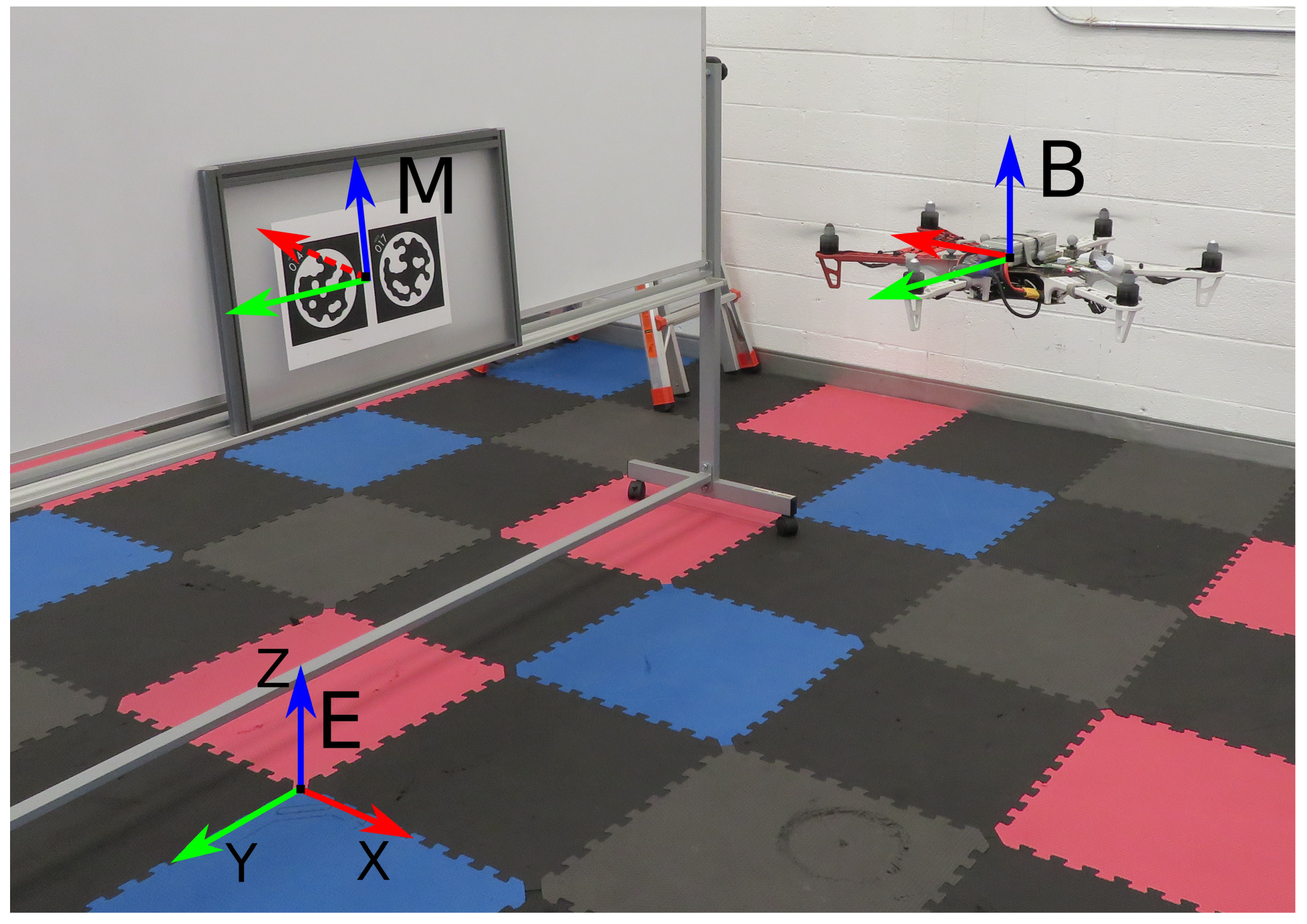
3.1. Lab Experiments

A hexrotor based on the DJI F550 was used for the lab experiments. The UAS was equipped with a Raspberry Pi 4B+ for all onboard processing and a second-generation piCam pointing toward the floor for fiducial marker tracking. Since the onboard computer had limited processing power, the NMPC horizon was set at 3 s and the control rate at 10 Hz. Nevertheless, the average OCP solution time was around 30 ms. The total weight of the UAS was 1.8 kg and the diagonal wheelbase was 550 mm. The system can be seen in Figure 3 during experimentation.
Since the proposed system was intended to be used in field experiments, an effort was made to mimic outdoor conditions inside the lab. First, wind disturbances were created using a leaf blower. Moreover, the MoCap position data were injected with artificial noise to generate virtual GNSS position data. GNSS position data are usually modeled as having both White and Brownian noise. Consequently, both types of noise were added to the MoCap position data. The added White noise reduced the overall accuracy of the MoCap measurements and the Brownian noise introduced a random walk bias. At time step k
p G N S S k = p M o C a p k + b k + ω , b k = b k 1 + υ ,
where p G N S S k is the virtual GNSS position used in the observer, p M o C a p k is the UAS position from the MoCap, ω N ( 0 , 10 3 ) is the additive White noise, and b k is the Brownian noise that is driven by υ N ( 0 , 10 3 ) .

3.1.1. Position Estimation

To test the position accuracy of the state estimation, the UAS was deployed and tasked with flying autonomously over a STag [37] fiducial marker bundle. The UAS could detect the fiducial marker bundle and track its pose [38]. The marker pose was then used by the state estimation to augment the platform’s position estimation. Figure 4 shows the generated GNSS position, the estimated position from the observer, and the real position of the system provided by the MoCap during a sample deployment. The UAS was tasked with hovering over the marker for around two minutes (129 s), and the marker was detected for 137 s. During the time that the marker was detected, the Root-Mean-Square (RMS) error for the generated GNSS position was 1.28 m. For the same time, the RMS error for the position provided by the filter was 0.13 m. Due to the limited power of the onboard computer used in this UAS, there were some gaps in the data, as the image processing required to detect the markers is an expensive process. However, the accuracy of the position acquired from the filter was significantly increased.

3.1.2. Disturbance Estimation

To test the effectiveness of the framework in estimating external disturbances and adapting to their effect, a similar experimental setup was used. The platform was again tasked with hovering over the marker, but this time, a leaf blower was used to generate wind disturbances (Figure 3), where the generated stream speed was measured using an anemometer. First, the leaf blower pushed the UAS toward the positive x-axis (maximum air-stream speed was 10 m/s), then toward the negative y-axis (maximum air speed was measured at 7 m/s), and finally, toward both the positive x-axis and negative z-axis (maximum stream speed of 10 m/s). Figure 5 shows the estimated disturbances during the deployment, and it is clear that the observer was able to estimate the disturbances. Moreover, the estimated direction and magnitude matched the applied disturbances. The magnitude of the first disturbance was around 1.5 and in the positive x-direction. The second disturbance was in the negative y-direction, with a magnitude of around 0.8 . Since the wind stream for the second disturbance was smaller than the first, it was expected that the estimated magnitude would be smaller as well. Finally, the last disturbance again exhibited the expected direction in both the x- and z-axes. Moreover, the magnitude on the x-axis was smaller than the first one, since the same wind gust was affecting two axes at the time.
The position of the UAS during the experiment can be seen in Figure 6. While the introduction of the wind disturbance affected the UAS position, the proposed framework could quickly adapt and return to the desired position. It is worth noting here the increased noise levels in the estimated position of the UAS, especially in the x- and y-axes. The camera of the drone was not rigidly mounted on the platform to reduce the effect of the motor and propeller vibrations on the acquired images. However, in the presence of significant winds, the camera mount moved relative to the UAS frame. This produced marker pose measurements with increased errors. Regardless, the RMS error during the autonomous portion of the flight was 13.2 cm, showing that the controller was capable of holding the desired position.

3.1.3. Trajectory Tracking

In the experimental setup described so far, the controller was tasked with hovering in place. In the next step, the controller was tested for its ability to also track desired trajectories. However, the setup of the indoor UAS experiment did not allow for tracking a stationary marker while moving around (as the UAS camera was fixed on the UAS frame). As such, the MoCap position was directly used by the state observer in the following experiments.
The first trajectory used was a simple back-and-forth trajectory. The UAS started on the positive x-axis and moved along the x-axis until it reached the negative edge before it turned back. At both edges, the trajectory included a 5 s stop. Two different iterations were considered for this trajectory. In the first iteration, a leaf blower was used to generate a wind stream toward the positive x-axis. The leaf blower was placed at the negative edge of the trajectory so that its nozzle was 1 m away. At the negative edge, the wind stream had a maximum velocity of 14.8 m/s, whereas at the positive edge, it was 5.5 m/s. The results of this deployment are shown in Figure 7. The RMS position error for this experiment was 7.6 cm. The UAS was able to track the desired trajectory, regardless of the significant wind disturbances. Moreover, the estimated disturbance increased when the UAS moved closer to the negative edge of the trajectory and then decreased while it moved away.
In the second iteration, the leaf blower was placed in the middle of the trajectory pointing toward the negative y-axis. At this point, the wind-stream velocity was 13.4 m/s. Compared to the previous setup, the UAS did not experience sustained wind but rather a sharp wind gust while it was passing through the middle of the trajectory. Figure 8 shows the results using this setup. The RMS position error for this experiment was 7.4 cm. One noticeable difference was that the platform was able to track the trajectory on the x-axis with reduced errors. Also, when the UAS was passing through the middle of the trajectory, the wind gust was registered by the observer, and the UAS was instantaneously pushed to the side before recovering.
Furthermore, an ascending spiral trajectory was used to test the controller. The radius of the spiral was set to 1 m; the starting and final altitudes were set to 0.75 m and 2.25 m, respectively; and the UAS had to complete three full rotations over 2 min. This trajectory required the platform to move on all three axes simultaneously. Moreover, the trajectory required that the UAS was always facing the center of the spiral. While the position of the platform was controlled by the NMPC, the orientation was controlled by a PID. Again, wind disturbances were introduced during the trajectory tracking as wind gusts when the drone was positioned at around (−1, 0). Four different wind conditions were used; no wind, side wind, side wind with around 20° pointing upwards, and finally, side wind with around 20° pointing downwards.
Figure 9 shows the results for the deployments under the various wind conditions examined. Although the drone was able to track the desired trajectory under all conditions, in the presence of strong wind gusts there was a drop in the platform’s attitude. This was the case regardless of the direction of the wind. Also, the highest tracking error occurred at the point where the disturbance was introduced. Specifically, the position RMS error for the full trajectory was 10.4 cm for the experiment without disturbances, 11.4 cm for the one with a direct side wind, 10.2 cm for the one with an upward-direction wind, and 9.2 cm for the one with a downward-direction wind. This indicates consistent performance despite the momentarily increased errors due to the wind gusts. Finally, although the position controller could accurately track the desired trajectory, the orientation controller experienced a constant offset error. This was due to the different controllers used for each task.

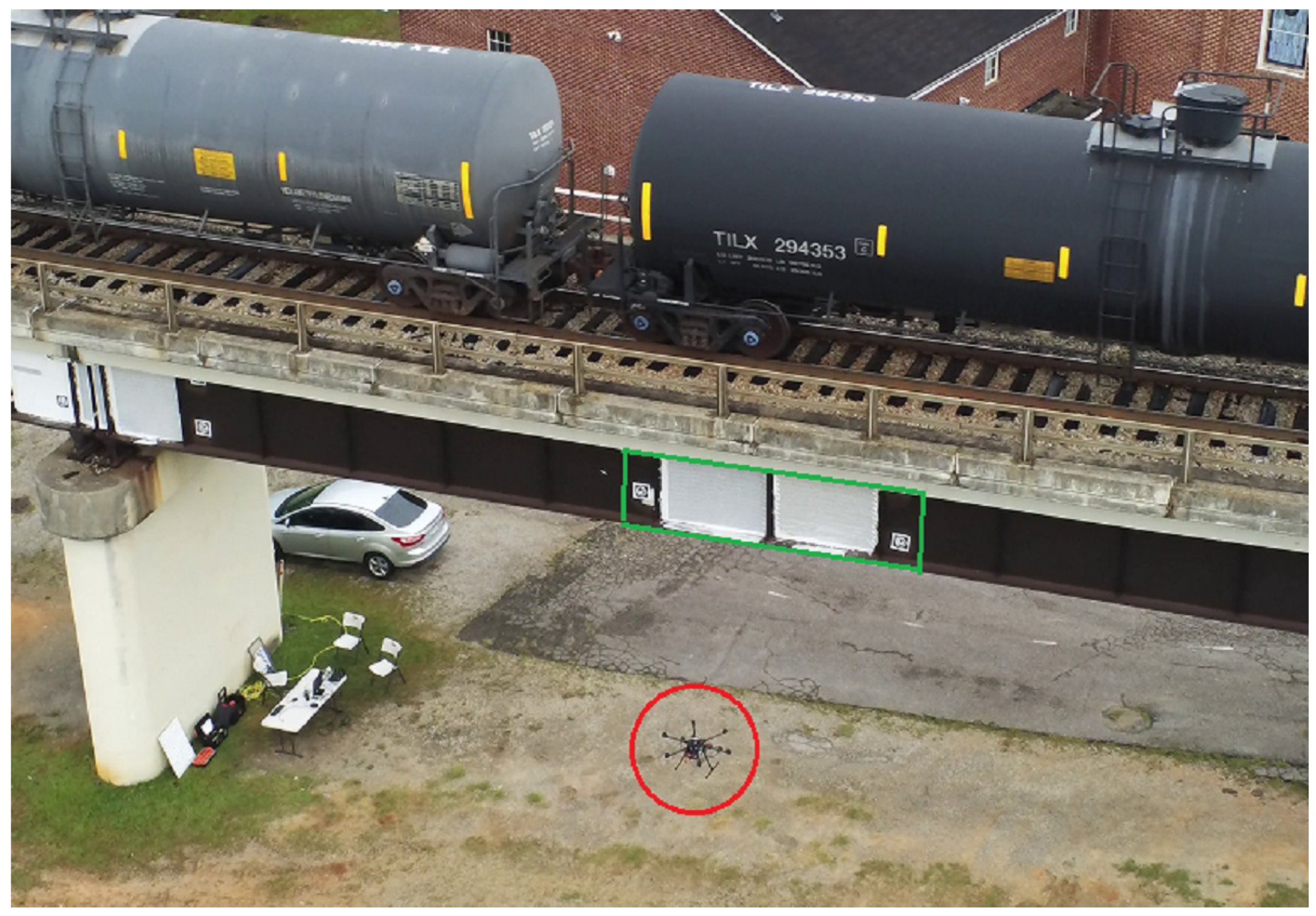
3.2. Field Experiments

For the field experiments, another UAS was used, namely the Aurelia X6 Standard platform. This is a much larger platform compared to the F550, with a total weight of 9.3 kg and a diagonal wheelbase of 1075 mm. The system is equipped with an Intel NUC i5 computer for onboard computing. Since this is a more powerful computer, the NMPC horizon was set at 3 s, the control rate at 20 Hz, and the average OCP solution time was around 15 ms. The system is also equipped with two 8.9-megapixel cameras that are used for both acquiring DIC inspection data [18] and tracking fiducial markers. Figure 10 shows the UAS during field deployment.
For the field experiment, the objective of the UAS was to hover steadily in a specific position relative to the inspection area. The inspection area was marked with a bundle of four STag markers that were also used to provide pose measurements. Figure 11 shows the position of the platform during a sample field deployment. The blue curve shows the position of the platform according to the GNSS and other avionics sensors, and the red curve shows the estimated position of the platform according to the developed state estimation framework. The black curve shows the desired position, and the vertical dashed lines show the portion of the flight that was autonomous. The drift of the GNSS position, which in a few cases was over a meter, is visible in the figure. Nevertheless, the developed state estimation framework used the model projections and the extra information from the marker to obtain a better estimation of the real position of the platform while tracking the GNSS random walk bias.
As for the developed controller, Figure 11 shows that it is able to keep the system close to the desired state. During the deployment shown in Figure 11, there were significant side winds; regardless, the controller was able to keep the platform in the desired position with an RMS error of 12 cm on the x-axis, 23 cm on the y-axis, and 16 cm on the z-axis. On the same day, the RMS error over five deployments with different wind conditions was 13 cm on the x-axis, 15 cm on the y-axis, and 22 cm on the z-axis.

4. Conclusions and Future Work

In this paper, we presented a UAS control framework that is robust to wind disturbances by estimating external disturbances and adapting its control. The framework is also robust to degraded GNSS signals by augmenting its pose estimation using data from fiducial markers. Rigorous experimental work, using two different UAS platforms in both indoor and field experiments, shows the effectiveness of the proposed framework. In all cases, the system exhibited consistent performance and error levels, regardless of the underlying conditions and the UAS platform used.
During experimentation, it was observed that the estimated external force in the zaxis was gradually increasing in magnitude in the negative direction. This can be seen in Figure 5. This was probably due to the decreasing battery power. The FCU maps the thrust to a specific signal sent to the motor controllers without considering the change in the available power. However, since the power changes, the same signal results in a lower thrust output. This, in turn, is registered by the state estimator as an increasing negative force. This can be improved by considering the battery level in the thrust equation of the model.
When neither the GNSS nor marker measurements are available, the state observer relies solely on using the system model and the attitude commands to propagate the state. In this case, however, the state observer is unable to estimate any external disturbances, while the estimation error due to unmodeled dynamics and modeling errors grows over time. Given enough time, the estimated state will become unreliable. In future work, the system will be able to monitor the uncertainty of the UAS position, and when it exceeds a safety level, it will either signal a safety pilot, if available, or try to move the UAS away from the structure.
While the focus of this work is to use the estimated external disturbances to adjust the position controller and achieve better performance, a possible extension is to use the same framework to estimate contact forces. This could be useful for UAS contact-based inspections [39] and sensor deployments [27,40] by allowing the UAS to apply the required force at the point of contact.

Author Contributions

Conceptualization, M.K. and N.V.; Formal analysis, N.V.; Funding acquisition, N.V.; Investigation, M.K. and N.V.; Methodology, M.K.; Project administration, N.V.; Software, M.K.; Supervision, N.V.; Validation, M.K.; Writing—original draft, M.K. and N.V.; Writing—review and editing, M.K. and N.V. All authors have read and agreed to the published version of the manuscript.

Funding

This work was partially funded by the University of South Carolina and the Federal Railroad Administration.

Data Availability Statement

The complete framework presented in this study, as well as scripts that implement the required system identification, are made publicly available at https://github.com/usrl-uofsc/px4_control.

Acknowledgments

The authors would like to thank Bhanuprakash Sairam Kosaraju for his help in running the experiments.

Conflicts of Interest

The authors declare no conflict of interest.

References

  1. Shakhatreh, H.; Sawalmeh, A.H.; Al-Fuqaha, A.; Dou, Z.; Almaita, E.; Khalil, I.; Othman, N.S.; Khreishah, A.; Guizani, M. Unmanned Aerial Vehicles (UAVs): A Survey on Civil Applications and Key Research Challenges. IEEE Access 2019, 7, 48572–48634. [Google Scholar] [CrossRef]
  2. Nooralishahi, P.; Ibarra-Castanedo, C.; Deane, S.; López, F.; Pant, S.; Genest, M.; Avdelidis, N.P.; Maldague, X.P.V. Drone-Based Non-Destructive Inspection of Industrial Sites: A Review and Case Studies. Drones 2021, 5, 106. [Google Scholar] [CrossRef]
  3. Jeong, K.; Kwon, J.; Do, S.L.; Lee, D.; Kim, S. A Synthetic Review of UAS-Based Facility Condition Monitoring. Drones 2022, 6, 420. [Google Scholar] [CrossRef]
  4. Lovelace, B.; Wells, J. Improving the Quality of Bridge Inspections Using Unmanned Aircraft Systems (UAS); Technical Report MN/RC 2018-26; Minnesota Department of Transportation: Saint Paul, MN, USA, 2018. [Google Scholar]
  5. Kim, I.H.; Yoon, S.; Lee, J.H.; Jung, S.; Cho, S.; Jung, H.J. A Comparative Study of Bridge Inspection and Condition Assessment between Manpower and a UAS. Drones 2022, 6, 355. [Google Scholar] [CrossRef]
  6. GPS Accuracy. Available online: https://www.gps.gov/systems/gps/performance/accuracy/ (accessed on 15 December 2022).
  7. Ameli, Z.; Aremanda, Y.; Friess, W.A.; Landis, E.N. Impact of UAV Hardware Options on Bridge Inspection Mission Capabilities. Drones 2022, 6, 64. [Google Scholar] [CrossRef]
  8. Zahran, S.; Moussa, A.; El-Sheimy, N. Enhanced Drone Navigation in GNSS Denied Environment Using VDM and Hall Effect Sensor. ISPRS Int. J. Geo-Inf. 2019, 8, 169. [Google Scholar] [CrossRef]
  9. Gyagenda, N.; Hatilima, J.V.; Roth, H.; Zhmud, V. A review of GNSS-independent UAV navigation techniques. Robot. Auton. Syst. 2022, 152, 104069. [Google Scholar] [CrossRef]
  10. Balamurugan, G.; Valarmathi, J.; Naidu, V.P.S. Survey on UAV navigation in GPS denied environments. In Proceedings of the 2016 International Conference on Signal Processing, Communication, Power and Embedded System (SCOPES), Paralakhemundi, India, 3–5 October 2016; pp. 198–204. [Google Scholar] [CrossRef]
  11. Petrlík, M.; Krajník, T.; Saska, M. LIDAR-based Stabilization, Navigation and Localization for UAVs Operating in Dark Indoor Environments. In Proceedings of the 2021 International Conference on Unmanned Aircraft Systems (ICUAS), Athens, Greece, 15–18 June 2021; pp. 243–251. [Google Scholar] [CrossRef]
  12. Waslander, S.; Wang, C. Wind Disturbance Estimation and Rejection for Quadrotor Position Control. In Proceedings of the AIAA Infotech@Aerospace Conference, Seattle, WA, USA, 6–9 April 2009. [Google Scholar] [CrossRef]
  13. Viktor, V.S.; Valery, I.F.; Yuri, A.Z.; Igor, S.; Denis, D. Simuation of wind effect on quadrotor flight. ARPN J. Eng. Appl. Sci. 2006, 10, 1535–1538. [Google Scholar]
  14. Mokhtari, A.; Benallegue, A. Dynamic feedback controller of Euler angles and wind parameters estimation for a quadrotor unmanned aerial vehicle. In Proceedings of the IEEE International Conference on Robotics and Automation, New Orleans, LA, USA, 26 April–1 May 2004; Volume 3, pp. 2359–2366. [Google Scholar] [CrossRef]
  15. Benallegue, A.; Mokhtari, A.; Fridman, L. High-order sliding-mode observer for a quadrotor UAV. Int. J. Robust Nonlinear Control 2008, 18, 427–440. [Google Scholar] [CrossRef]
  16. Alexis, K.; Nikolakopoulos, G.; Tzes, A. Model predictive quadrotor control: Attitude, altitude and position experimental studies. IET Control Theory Appl. 2012, 6, 1812–1827. [Google Scholar] [CrossRef]
  17. Kalaitzakis, M.; Kattil, S.R.; Vitzilaios, N.; Rizos, D.; Sutton, M. Dynamic Structural Health Monitoring using a DIC-enabled drone. In Proceedings of the 2019 International Conference on Unmanned Aircraft Systems (ICUAS), Atlanta, GA, USA, 11–14 June 2019; IEEE: Piscataway, NJ, USA, 2019. [Google Scholar] [CrossRef]
  18. Kalaitzakis, M.; Vitzilaios, N.; Rizos, D.C.; Sutton, M.A. Drone-Based StereoDIC: System Development, Experimental Validation and Infrastructure Application. Exp. Mech. 2021, 61, 981–996. [Google Scholar] [CrossRef]
  19. PX4 Open Source Autopilot. Available online: https://px4.io/ (accessed on 15 December 2022).
  20. Quigley, M.; Gerkey, B.; Conley, K.; Faust, J.; Foote, T.; Leibs, J.; Berger, E.; Wheeler, R.; Ng, A. ROS: An open-source Robot Operating System. In Proceedings of the ICRA Workshop on Open Source Software, Kobe, Japan, 12–17 May 2009. [Google Scholar]
  21. Yuksel, B.; Secchi, C.; Bulthoff, H.H.; Franchi, A. A nonlinear force observer for quadrotors and application to physical interactive tasks. In Proceedings of the 2014 IEEE/ASME International Conference on Advanced Intelligent Mechatronics, Besacon, France, 8–11 July 2014. [Google Scholar] [CrossRef]
  22. McKinnon, C.D.; Schoellig, A.P. Unscented external force and torque estimation for quadrotors. In Proceedings of the 2016 IEEE/RSJ International Conference on Intelligent Robots and Systems (IROS), Daejeon, Republic of Korea, 9–14 October 2016; pp. 5651–5657. [Google Scholar] [CrossRef]
  23. Al-Radaideh, A.; Sun, L. Self-Localization of Tethered Drones without a Cable Force Sensor in GPS-Denied Environments. Drones 2021, 5, 135. [Google Scholar] [CrossRef]
  24. Tomic, T.; Haddadin, S. Simultaneous estimation of aerodynamic and contact forces in flying robots: Applications to metric wind estimation and collision detection. In Proceedings of the 2015 IEEE International Conference on Robotics and Automation (ICRA), Seattle, WA, USA, 26–30 May 2015; pp. 5290–5296. [Google Scholar] [CrossRef]
  25. Tomić, T. Model-Based Control of Flying Robots for Robust Interaction under Wind Influence; Springer International Publishing: Berlin/Heidelberg, Germany, 2023. [Google Scholar] [CrossRef]
  26. Ljung, L. System Identification. In Signal Analysis and Prediction; Birkhäuser Boston: Boston, MA, USA, 1998; pp. 163–173. [Google Scholar] [CrossRef]
  27. Kalaitzakis, M.; Kosaraju, B.S.; Vitzilaios, N. Efficient UAS sensor mounting using contact force feedback. In Proceedings of the 2023 International Conference on Unmanned Aircraft Systems (ICUAS), Warsaw, Poland, 6–9 June 2023; pp. 313–319. [Google Scholar] [CrossRef]
  28. Solà, J. Quaternion Kinematics for the Error-State Kalman Filter. arXiv 2017, arXiv:1711.02508. [Google Scholar] [CrossRef]
  29. Madyastha, V.; Ravindra, V.; Mallikarjunan, S.; Goyal, A. Extended Kalman Filter vs. Error State Kalman Filter for Aircraft Attitude Estimation. In Proceedings of the AIAA Guidance, Navigation, and Control Conference, Portland, OR, USA, 8–11 August 2011. [Google Scholar] [CrossRef]
  30. Roumeliotis, S.; Sukhatme, G.; Bekey, G. Circumventing dynamic modeling: Evaluation of the error-state Kalman filter applied to mobile robot localization. In Proceedings of the 1999 IEEE International Conference on Robotics and Automation, Detroit, MI, USA, 10–15 May 1999; pp. 1656–1663. [Google Scholar] [CrossRef]
  31. Mehra, R. Approaches to adaptive filtering. IEEE Trans. Autom. Control 1972, 17, 693–698. [Google Scholar] [CrossRef]
  32. Hausman, K.; Weiss, S.; Brockers, R.; Matthies, L.; Sukhatme, G.S. Self-calibrating multi-sensor fusion with probabilistic measurement validation for seamless sensor switching on a UAV. In Proceedings of the 2016 IEEE International Conference on Robotics and Automation (ICRA), Stockholm, Sweden, 16–21 May 2016; pp. 4289–4296. [Google Scholar] [CrossRef]
  33. Chiella, A.C.B.; Teixeira, B.O.S.; Pereira, G.A.S. State Estimation for Aerial Vehicles in Forest Environments. In Proceedings of the 2019 International Conference on Unmanned Aircraft Systems (ICUAS), Atlanta, GA, USA, 11–14 June 2019; pp. 890–898. [Google Scholar] [CrossRef]
  34. Kamel, M.; Stastny, T.; Alexis, K.; Siegwart, R. Model Predictive Control for Trajectory Tracking of Unmanned Aerial Vehicles Using Robot Operating System. In Studies in Computational Intelligence; Springer International Publishing: Berlin/Heidelberg, Germany, 2017; pp. 3–39. [Google Scholar] [CrossRef]
  35. Houska, B.; Ferreau, H.; Diehl, M. ACADO Toolkit—An Open Source Framework for Automatic Control and Dynamic Optimization. Optim. Control Appl. Methods 2011, 32, 298–312. [Google Scholar] [CrossRef]
  36. Houska, B.; Ferreau, H.; Diehl, M. An Auto-Generated Real-Time Iteration Algorithm for Nonlinear MPC in the Microsecond Range. Automatica 2011, 47, 2279–2285. [Google Scholar] [CrossRef]
  37. Benligiray, B.; Topal, C.; Akinlar, C. STag: A stable fiducial marker system. Image Vis. Comput. 2019, 89, 158–169. [Google Scholar] [CrossRef]
  38. Kalaitzakis, M.; Cain, B.; Carroll, S.; Ambrosi, A.; Whitehead, C.; Vitzilaios, N. Fiducial Markers for Pose Estimation. J. Intell. Robot. Syst. 2021, 101, 71. [Google Scholar] [CrossRef]
  39. Bodie, K.; Brunner, M.; Pantic, M.; Walser, S.; Pfndler, P.; Angst, U.; Siegwart, R.; Nieto, J. An Omnidirectional Aerial Manipulation Platform for Contact-Based Inspection. In Proceedings of the Robotics: Science and Systems XV, Breisgau, Germany, 22–26 June 2019. [Google Scholar] [CrossRef]
  40. Carroll, S.; Kalaitzakis, M.; Vitzilaios, N. UAS Sensor Deployment and Retrieval to the Underside of Structures. In Proceedings of the 2021 International Conference on Unmanned Aircraft Systems (ICUAS), Athens, Greece, 15–18 June 2021; pp. 895–900. [Google Scholar] [CrossRef]
Figure 1. A model UAS with the attached body frame B, the fixed inertial frame E, and a fiducial marker-attached frame M.
Robotics 12 00123 g001
Figure 2. Control system architecture.
Robotics 12 00123 g002
Figure 3. Indoor lab experiments using a small UAS, where a leaf blower was used to produce wind disturbances.
Robotics 12 00123 g003
Figure 4. The three plots show the UAS position during deployment, in the x, y, and z axis, respectively. The virtual GNSS is in green, the state observer is in blue, and the MoCap system is in red. The vertical dashed lines show the first and last times the marker was detected.
Robotics 12 00123 g004
Figure 5. The external disturbances, as estimated using the proposed framework while hovering.
Robotics 12 00123 g005
Figure 6. UAS position measurements during the hovering task and while being affected by the wind disturbances shown in Figure 5.
Robotics 12 00123 g006
Figure 7. The UAS position and estimated disturbance along the x-axis during a back-and-forth trajectory, with a face wind.
Robotics 12 00123 g007
Figure 8. The UAS position along the x and y axes, and the estimated disturbance along the y-axis during a back-and-forth trajectory, with a side wind in the middle of the trajectory.
Robotics 12 00123 g008
Figure 9. The UAS position and orientation during the spiral trajectories under all four different wind conditions.
Robotics 12 00123 g009
Figure 10. The UAS used for field deployments during a railroad bridge inspection. The UAS is highlighted with a red circle, and the inspection area is highlighted with a green box.
Robotics 12 00123 g010
Figure 11. The position of the platform during one of the field deployments. The red curve shows the estimated position from the developed state observer, whereas the blue curve shows the reported position from the avionics sensors. The black curve shows the desired position, and the dashed vertical lines show the autonomous portion of the flight.
Robotics 12 00123 g011
Table 1. The ESKF variables.
TrueNominalErrorComposition
UAS position p D t r u e p D δ p D p D t r u e = p D + δ p D
UAS velocity v D t r u e v D δ v D v D t r u e = v D + δ v D
UAS attitude q D t r u e q D δ q D q D t r u e = q D δ q D
Angles vector δ θ δ q D = e δ θ / 2
Disturbances F t r u e F δ F F t r u e = F + δ F
Marker position p M t r u e p M δ p M p M t r u e = p M + δ p M
Marker attitude q M t r u e q M δ q M q M t r u e = q M δ q M
GNSS bias b t r u e b δ b b t r u e = b + δ b
Disclaimer/Publisher’s Note: The statements, opinions and data contained in all publications are solely those of the individual author(s) and contributor(s) and not of MDPI and/or the editor(s). MDPI and/or the editor(s) disclaim responsibility for any injury to people or property resulting from any ideas, methods, instructions or products referred to in the content.

