Non-Prehensile Manipulation Actions and Visual 6D Pose Estimation for Fruit Grasping Based on Tactile Sensing ^†

Abstract

Robotic manipulation in cluttered environments is one of the challenges roboticists are currently facing. When the objects to handle are delicate fresh fruits, grasping is even more challenging. Detecting and localizing fruits with the accuracy necessary to grasp them is very difficult due to the large variability in the aspect and dimensions of each item. This paper proposes a solution that exploits a state-of-the-art neural network and a novel enhanced 6D pose estimation method that integrates the depth map with the neural network output. Even with an accurate localization, grasping fruits with a suitable force to avoid slippage and damage at the same time is another challenge. This work solves this issue by resorting to a grasp controller based on tactile sensing. Depending on the specific application scenario, grasping a fruit might be impossible without colliding with other objects or other fruits. Therefore, a non-prehensile manipulation action is here proposed to push items hindering the grasp of a detected fruit. The pushing from an initial location to a target one is performed by a model predictive controller taking into account the unavoidable delay in the perception and computing pipeline of the robotic system. Experiments with real fresh fruits demonstrate that the overall proposed approach allows a robot to successfully grasp apples in various situations.

1. Introduction

One of the most important human skills that robots try to emulate is the capability to manipulate objects with great agility and ease. In fact, a classic robotic task consists in moving an object from one place to another, also in a cluttered environment. To do this, typically, a pick-and-place approach is adopted: the robotic manipulator is equipped with a sensorized gripper used by the robot to grasp the object, lift it and move it to another location [1]. However, this solution is not versatile enough to be used in all contexts. Depending on the gripper design, if the object is too large or too small or too heavy, it can be unsuitable. Moreover, if the environment is cluttered and the object is occluded by others, the grasp may fail. But observing how humans interact with objects, it is the same: if we have to move a heavy object, we prefer to use a non-prehensile manipulation, such as pushing, rather than grasping and lifting it. And if we have to pick an object in a cluttered box, we push all the obstacles that make it difficult for us to grasp the desired object before grasping it. In fact, for humans using both prehensile and non-prehensile manipulation actions is natural and, depending on the context, the latter can even be preferred to the former. Therefore, a robot manipulator might use both prehensile and non-prehensile manipulations to come close to the same human dexterity. This paper focuses on pushing, a non-prehensile solution that expands the robotic skills in the manipulation field. The dynamics of pushing is highly nonlinear and it is dominated by the frictional forces, which are typically difficult to measure, making predicting the motion of the pushed object on an arbitrary surface hard. In fact, the result of a physical interaction between a robot and an object, i.e., pushing through a contact point, depends on physical laws, which are challenging to model. For example, depending on the physical parameters, a pushed object may rotate or translate or both, with a motion difficult to predict. Nevertheless, the pushing primitive can be used to resolve many problems [2]: positioning and orienting objects in the plane, facilitating their grasping, estimating their pose and their shape [3], identifying some inertial parameters, such as the friction coefficient [4].

This work, in particular, studies the problem of pushing an object from an arbitrary start position to a target one on a flat surface with a robotic arm. Technically, it deals with the so-called planar pushing with one contact point under the quasi-static assumption [5]. Several researchers have solved this problem by generating open-loop plans, which do not require feedback sensing, as in [6]. However, the unpredictable behavior of a sliding object on a surface and most of all the impossibility to know exactly the system parameters, such as coefficients of friction (between the object and the support surface and between the pusher and the object), require the use of feedback. In fact, like for humans, for robotic manipulators processing information from sensing is the only way to recover and correct their motion. Typically, the pushing control system is based on visual feedback used to the pose of the pushed object, or on tactile feedback, as in [7], in which force measurements are used to control the interaction between the slider and the pusher. Anyway, the design of feedback controllers for the pusher–slider system based on frictional contact interactions is made more difficult by two characteristic challenges of robotic manipulation tasks: the hybridness and the underactuation [8]. The former arises from the multiple contact modes between the pusher and the pushed object (e.g., sticking and sliding): switching from one mode to another results in a discontinuity in the dynamics, making the controller design more difficult. The latter arises from nonholonomic constraints, i.e., not integrable constraints on the velocity of the pushed object, caused by the limitation on the force direction applicable by the pusher [1]. A model predictive control approach seems to be the most suitable to model the dynamic constraints as well as the hybrid nature of the contact. Among the several solutions, this paper is inspired to the approach proposed in [9], in which a model predictive control approach is mixed with an integer programming and optimized with the so-called Family of Modes (FOM) concept to achieve a real-time control.

The paper is organized as follows. We begin by reviewing the main approaches used to realize robotic pushing (Section 1.1) and the state-of-the-art methods for the 6D pose estimation (Section 1.2). In Section 2, we briefly describe the approach used to recover the 6D pose from visual information, as developed in [10]. We then proceed with the description of the pushing control system proposed in [9], highlighting the proposed improvements to their solution (Section 3). Section 4.1 summarizes the overall pick-and-place pipeline already developed in [10] and here extended with a non-prehensile manipulation. Finally, in Section 5, we describe several experiments to validate the enhanced pushing approach described in the previous section. In detail, the experiments presented in the paper show how a non-prehensile manipulation can be used as pre-grasp operation to pick a fruit occluded by another object that cannot be directly grasped due to scene constraints, i.e., gripper design, object shape, and further obstacles. Indeed, the problem of fruit manipulation, already addressed in [10], is placed in a more complex context, in which other robotic manipulations are required to successfully complete the proposed task of picking a fruit without damaging it.

1.1. Related Work on Robotic Pushing

The problem of planar pushing has always been a very active research topic in robotics for its importance as part of robotic manipulation. It was analyzed for the first time in 1986 by Mason under the quasi-static hypothesis [5]. This assumption is typical for robotic manipulation actions and consists of assuming that pusher motions are slow enough that inertial forces are negligible compared to frictional forces. Full descriptions of the interaction forces are rarely considered.

Mason approached the problem analytically, and relying on the relevant theory of sliding friction and classical mechanics, he developed analytical tools to plan a pushing manipulation to achieve the desired outcome. In [5], Mason derived the voting theorem, a rule for determining the sense of rotation of a pushed object depending on its centre-of-mass, without an explicit knowledge of the pressure distribution between the object and its support surface. This is a very important result, considering that the distribution of pressure at the contact between the object and the supporting surface is difficult to estimate, and consequently, the frictional forces arising at the contact are indeterminate [11]. Following that, an important contribution was offered by Goyal et al.: in [12], they studied the resultant of the frictional contact forces when the support forces are given and they introduced the limit surface (LS) concept to provide a geometric description of the net frictional force and moment between the rigid body and a planar surface on which it slides. Although the limit surface has been successfully used in feedback control applications under the quasi-static assumption, it was computationally expensive due to the lack of a convenient form to construct it. To reduce the computational time needed to compute it, Lee and Cutkosky in [13] generalized the concept of the limit surface for irregular pressure distribution and, relying on the knowledge of pressure distribution, derived the so-called ellipsoidal approximation. It provides an invertible relationship between motions and forces. Then, it was used by Lynch et al. [7] to develop a model of the motion of a pushed object, which can be used in the design of a pushing controller. Under the assumption of quasi-static interactions, they derived an analytical mapping between pusher and object velocities.

These results have been used for planning and controlling the pushing operation with a robotic manipulator. Among the most famous works, Lynch and Mason in [1] analyzed three issues in pushing, i.e., mechanics, controllability, and planning, to develop planning algorithms to automatically find stable pushing paths among obstacles.

However, due to the high complexity of the problem, the analytical approach, used to derive a model of the physical contact between the object pushed and the pusher, relies on some modeling assumptions that are not always verified in reality, e.g., the uniform distribution of friction on a surface. The mismatch between the modeling and the real-world conditions affects the proper behavior of the system. For these reasons, in recent years, researchers have extended the analytic approach with data-driven methods, i.e., the interaction between the objects is still described with an analytical model, but some critical parameters are estimated by experiments and learned by a large amount of collected data. This allows to avoid strong or minor hypothesis on the involved physical parameters. In [14], the authors try to better capture frictional interactions with a data-driven approach: they use a Gaussian regression to learn the model and show that the resulting system can be controlled through a model predictive control. In [15], the authors use a density estimation model with a data-driven approach to predict the motion of a rigid object resulting from a robotic push.

Although data-driven approaches enjoy high flexibility with less restrictive assumptions, they require a large amount of data and their recording is very time-consuming. Both analytical and data-driven approaches described so far are model-based, but recently there has been a growing interest in reinforcement learning, thanks to which a model-free approach can be used to overcome all the problems aforementioned. In [16], a deep neural network is used to model the motion of a rigid object pushed by a robot on a surface through raw point cloud data. They try to learn dynamics from a visual stream: the network takes depth images as input, splits point clouds into pieces of the object, and predicts their motion in terms of SE(3) transformations. In [17], a model-free reinforcement learning is used to discover and learn the utility of pushes combined with the grasp. The authors focus on the benefits for robotic manipulation coming from the synergies between non-prehensile and prehensile actions. They trained two fully convolutional networks, one for pushing and the other for grasping, in a Q-learning framework, self-supervised by trial and error. With picking experiments they show that their method achieves a higher grasping success rate, thanks to the use of pushing when deemed necessary by the learning framework.

Although these latter and more advanced methods appear to be promising, planar pushing remains challenging for learning-based control approaches, as much as for the model-based ones. This paper exploits a model-based approach to design a model predictive controller that, differently from existing solutions based on the same strategy, explicitly takes into account the communication delay of the digital implementation and exploits a novel perception pipeline to detect, localize and track the pushed object. Furthermore, the method has been generalized to allow the robot to push a given object along a generic trajectory rather than a straight line only, while ensuring a smooth motion.

With reference to the literature reviewed so far on the non-prehensile manipulation, the key aspects of our improvements of the state-of-the-art model-based approach for robotic pushing, proposed in [9], are:

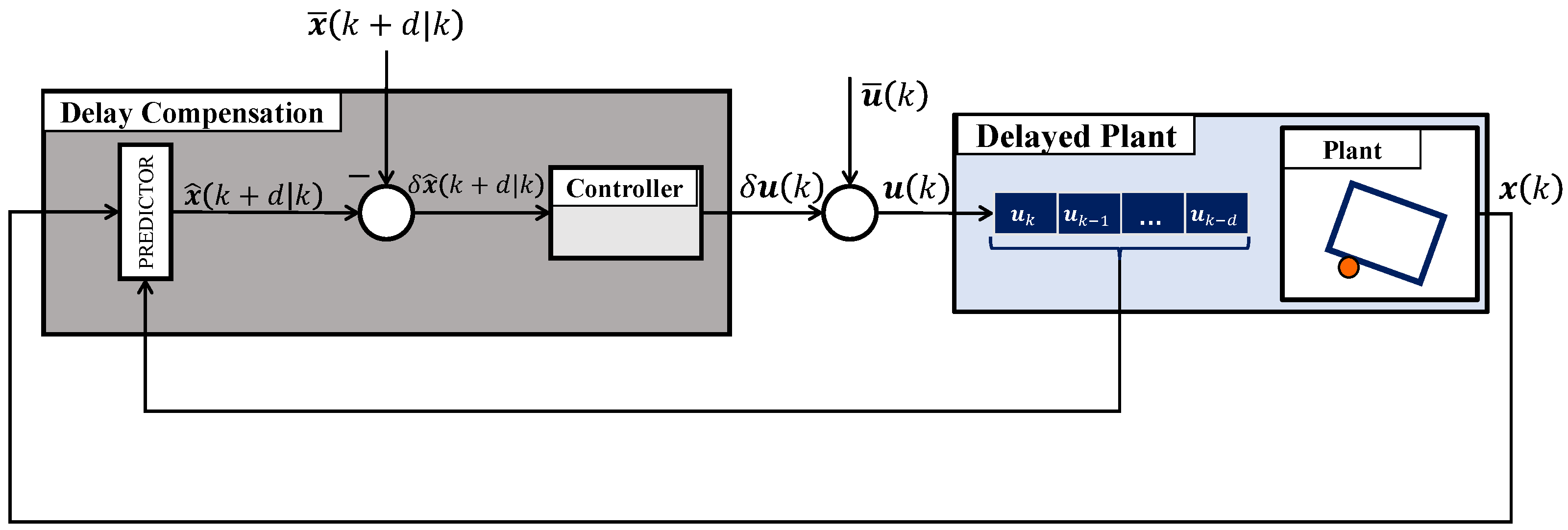
• A compensation delay strategy to make the control system able to reach the desired goal with the expected performance despite the delays arising from a digital implementation of the perception and communication pipeline;
• A chattering avoidance strategy to reduce as much as possible the oscillations in high frequency arising from the hybrid nature of the considered system;
• A novel trajectory generation approach to make the control system design independent of the particular trajectory to be tracked.

1.2. Related Work on Object Detection

One of the main challenges that must be addressed in the realization of a robotic food-handling solution is the estimation of the position and orientation of the objects in the space, i.e., their 6D pose. Indeed, the success of the robotic solution first depends on its ability to detect and localize foods in the surrounding environment, independently from their wide variability in appearance, dimension, and shape.

The approaches to the 6D pose estimation problem can be categorized in several ways; commonly accepted classifications are the instance level and category level methods.

Instance-level methods assume an exact 3D CAD model is available during training and they expect to work on the same instance object during inference. They can be further divided into template-based and regression-based methods. Template-based methods use a set of template images of the object instance captured from different views and then compare them to the input image at run-time. They have demonstrated impressive results in terms of accuracy and speed, working well also for texture-less objects, but often performance degrades when the objects are partially occluded [18,19,20]. Regression-based methods can directly estimate the 6D pose, as PoseCNN [21], or predict 2D projected key-points, which are then used by the PnP algorithm to solve the 6D pose as in DOPE [22] and MobilePose [23]. Both the approaches cited above work well when the inference is performed on the same instance on which they have been trained, but performance deteriorates when the target object little differs from the 3D model, so they suffer from a lack of scalability, e.g., if one is trained on a brand of a fruit juice it will not recognize the fruit juice of another brand. Convolutional neural networks, as for many problems of computer vision, are a widespread solution for 6D pose estimation problems. In this case, the instance level methods can use to their advantage the knowledge of the 3D CAD model to easily generate a large synthetic dataset for the training. Indeed, the realization of a dataset for 3D object detection with real-world images manually labeled is very time-consuming, labor-intensive and error-prone. On the other hand, networks trained only on synthetic data degrade when used on real data due to the so-called reality-gap problem.

Category-level methods instead focus on object recognition within a specific category and so do not require a 3D CAD model. In CenterPose [24], Tremblay et al. propose a single-stage, keypoint-based approach for object pose estimation that operates on unknown object instances within a known category using a single RGB image as input. In [25], semantic keypoints predicted by a convolutional network are combined with a deformable shape model to recover the 6D pose, making no distinction between textured and texture-less objects. The main drawback of these methods is the need of large datasets realized with real-world images, due to the absence of a 3D model. Some more recent works try to overcome this shortcoming as in NOCS [26], where a mixed reality method to automatically generate large amounts of data for category level recognition is proposed, or CPS++ [27] and Self6D [28], which proposes the idea of synthetic-to-real domain transfer for class-level 6D poses through self-supervised learning.

To recognize fruits and vegetables, category-level methods would be more suitable due to the great intra-class variability of the target objects. Nevertheless, the collection of a rich dataset with real images for each class, including as many as possible variations in lights, environments, and viewpoints, for each object in the specific category, is not feasible, and, to the best of our knowledge, the category level methods that try to merge synthetics data and class recognition are still too young. Therefore, to take the great advantage of synthetic data generation, the instance level method DOPE [22] has been chosen for the recognition step of the robotic picking system, enhanced with the method presented in [10] and briefly recalled in Section 2.

Owing to the accurate localization offered by the proposed method, the grasp is likely to be successful as proved by the results discussed in the next section. Nevertheless, real-world fruits and vegetables vary in shape, size, weight, and friction, hence the handling phase of each actual item is non-trivial. This issue can be tackled by resorting to tactile sensing in combination with a state-of-the-art grasp force control algorithm. Specifically, we adopt the SunTouch tactile sensors [29] and the model-based slipping control algorithm originally presented in [30] and extended in [31]. The main idea behind this approach is to estimate the slipping velocity by means of a nonlinear observer and regulate it to zero. This way it is possible to automatically modulate the grasping force without knowing the weight of the handled item while also reacting to external disturbances, e.g., unforeseen collisions with obstacles that might cause fruit drops.

With respect to the detection and 6D localization methods reviewed so far, for the detection of fresh fruits, we adopt here a method, originally presented in [10], enhancing a state-of-the-art neural network that cannot deal with the significant variability of fruits of the same species and provides a 6D pose of the fruit with an accuracy not sufficient to perform a correct picking. Our method is such that the estimated pose accuracy is independent of the fruit dimensions, which can vary significantly even for given species of fruit.

2. Object Recognition and 6D Localization

The proposed object recognition and 6D localization algorithm is based on a state-of-the-art deep neural network for 6D pose estimation, i.e., DOPE [22], followed by the pose refinement algorithm that addresses the problem of dimensions variability of the target objects, proposed in [10].

The adopted deep neural network, DOPE, belongs to the instance-level and regression-based category. It infers, in near real-time, the poses of known rigid objects in a cluttered environment from a single RGB image without requiring post-alignment. The authors showed how their network, trained only on synthetic data without fine-tuning, achieves state-of-the-art performance on 6D object pose estimation, promising a great solution to speed up the training process of such networks.

The algorithm first regresses the nine keypoints of a cuboid enclosing the recognized object, i.e., its eight vertices and centroid, and then passes them to the PnP algorithm [32], that, given the camera intrinsics and the CAD cuboid dimensions, is able to retrieve the 6D object pose.

When the network is used to recognize objects that are scaled versions of the CAD model used during the training, the resulting estimated pose is affected by a positioning error depending on the scale difference between the real object and the CAD model. To overcome this limitation, a pose refinement algorithm, described in [10] and shortly summarized for self-consistency in Section 2.2, is adopted. By using the pose estimated by DOPE, the CAD model used during the training, and the depth map provided by an RGB-D sensor, an optimization problem is resolved to obtain the refined pose.

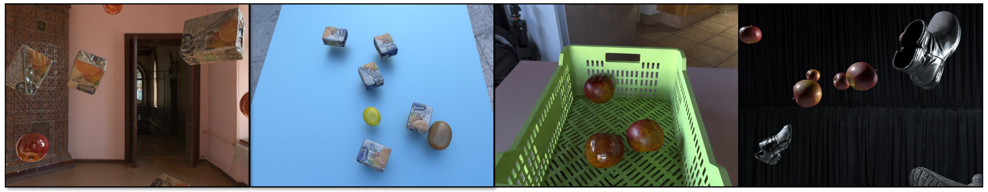
2.1. Network Training

The DOPE network has been trained to recognize two objects: a specific fruit juice brick and a red apple. While for the first one, an exact CAD model was available, for the second one a generic CAD model has been used for obvious reasons.

Following the approach described in [22], both domain randomized (DR) and photo realistic (PR) images have been synthesized for the dataset creation.

For both objects, DR data were generated by placing in virtual worlds a random number of object instances in arbitrary positions and orientations along with an arbitrary number of distractors (selected from a set of 3D models). For each simulation, the environment, the light conditions, and the applied noise are randomly chosen. Once all is set up, forces and moments of random intensities and directions are applied to each object in the scene. As a result, objects will move in the scene in a chaotic manner, colliding and overlapping each other. A camera, in a fixed position, takes pictures of the scene at a fixed rate along with the annotations for the training.

The PR data, instead, have been generated by placing the objects on a table or in a fruit crate (in the case of apples) in a realistic way. The annotated images are then captured with a camera that moves around the table with a variable elevation and inclination. Each time a virtual world is created in this manner, a number of parameters are randomly chosen, such as the number of objects and distractors, their poses, the light conditions, the color and the dimension of the table (fruit crate), and the camera maximum elevation and inclination. Figure 1 shows some images of the dataset generated with the NVISII tool [33].

Table 1. Training parameters for the two DOPE networks.

Training parameters for the juice brick
DR frames	$\sim 50$ k
PR frames	$\sim 10$ k
epochs	70
learning rate	$0.0001$
train batch size	116
test batch size	32
optimizer	Adam
training time	$\sim 2$ days
Training parameters for the red apple
DR frames	$\sim 100$ k
PR frames	$\sim 20$ k
epochs	120
learning rate	$0.0001$
train batch size	116
test batch size	32
optimizer	Adam
training time	$\sim 3$ days

reports the training parameters of the two networks used for detecting the juice brick and the red apple.

2.2. Pose Refinement

The instance-level inference system adopted to detect fruits and vegetables is prone to positioning errors in case the object to detect is scaled bigger or smaller than the one used to train the network, which is a likely circumstance for fresh fruits. DOPE will interpret the scale difference as a translation, farthest or closest, of the target object. Indeed, an object seen from a 2D camera can be interpreted in an equivalent way as a smaller version of the same object placed closer to the camera or a larger version placed further away. To address this shortcoming for an object of unknown dimensions, a method able to translate and scale an object without altering its representation in the image plane of the camera is summarized in this section for self-consistency of the present manuscript even though proposed in [10].

Let the estimated object pose by DOPE be represented by the vector $\widehat{\mathit{p}}$ and the unit quaternion $\widehat{\mathit{Q}}$ indicating the position and the orientation of the recognized object with respect to the camera frame, respectively. Placing the CAD model used for the training in a virtual world at the position $\widehat{\mathit{p}}$ and orientation $\widehat{\mathit{Q}}$, with respect to the camera frame (of a virtual camera), a virtual depth map can be acquired and compared with the one coming from the real RGB-D sensor. The idea is to translate the CAD model in the new position ${\mathit{p}}^{\prime }$ without changing its orientation and to scale it into the updated cuboid dimensions ${\mathit{d}}^{\prime }$ so that its RGB image, captured by the virtual sensor, is the same, while the corresponding virtual depth map is different. The updated values ${\mathit{p}}^{\prime }$ and ${\mathit{d}}^{\prime }$ are evaluated as

$${\mathit{p}}^{\prime }=\widehat{\mathit{p}}-\sigma \frac{\widehat{\mathit{p}}}{∥\widehat{\mathit{p}}∥}$$

(1)

$${\mathit{d}}^{\prime }=\mu \left(\sigma \right){\mathit{d}}_{CAD},\mathrm{with}\mu \left(\sigma \right)=\frac{∥{\mathit{p}}^{\prime }∥}{∥\widehat{\mathit{p}}∥},$$

(2)

where $\sigma$ is a scalar factor, $\mu \left(\sigma \right)$ is a scale factor depending on $\sigma$ and ${\mathit{d}}_{CAD}={\left[\begin{array}{c}{d}_x{d}_y{d}_z\end{array}\right]}^T$ denotes the CAD cuboid dimensions. Starting from these equations, a cost function depending on $\sigma$ can be defined and minimized, as described in [10].

The optimum ${\sigma }_{opt}$, obtained by solving the optimization problem, is such that the depth map coming from the RGB-D sensor and the one rendered, are best overlapped. Therefore, it is used in (1) and (2) to obtain the refined position and the estimated real cuboid dimensions.

The pose refinement algorithm is validated through experimental results, as discussed in detail in [10], and here briefly recalled for the reader’s convenience. Five red apples of significantly different dimensions were placed in five different locations on the table where the robot was mounted. For each apple and each location, three grasp attempts were made, firstly, only using the pose coming from DOPE (

Table 2. Grasping success rate without pose refinement.

	ATT. 1	ATT. 2	ATT. 3	ATT. 4	ATT. 5
Apple 1	$100\%$	$66\%$	$0\%$	$100\%$	$100\%$
Apple 2	$33\%$	$33\%$	$33\%$	$0\%$	$0\%$
Apple 3	$66\%$	$33\%$	$33\%$	$33\%$	$33\%$
Apple 4	$0\%$	$0\%$	$0\%$	$0\%$	$0\%$
Apple 5	$0\%$	$0\%$	$0\%$	$0\%$	$0\%$

), and secondly, refining the pose with the novel algorithm (

Table 3. Grasping success rate with pose refinement.

	ATT. 1	ATT. 2	ATT. 3	ATT. 4	ATT. 5
Apple 1	$100\%$	$100\%$	$100\%$	$100\%$	$100\%$
Apple 2	$100\%$	$100\%$	$100\%$	$100\%$	$100\%$
Apple 3	$66\%$	$66\%$	$100\%$	$100\%$	$100\%$
Apple 4	$66\%$	$100\%$	$100\%$	$100\%$	$100\%$
Apple 5	$66\%$	$33\%$	$66\%$	$66\%$	$66\%$

). The comparison of Table 2 and Table 3 shows that the pose refinement algorithm significantly increases the grasping success rate.

3. Pushing Control

In the experiments used to validate the perception pipeline, the environment was static and there were no objects impeding the grasp maneuver. In order to improve the autonomy of the robotic system shown so far and to make grasping feasible even if the objects collide with each other, a control system for the execution of non-prehensile robotic manipulation actions has been designed. In particular, we focus on a pushing maneuver and we will show how it can be used as a pre-grasp manipulation to make the desired prehensile one feasible.

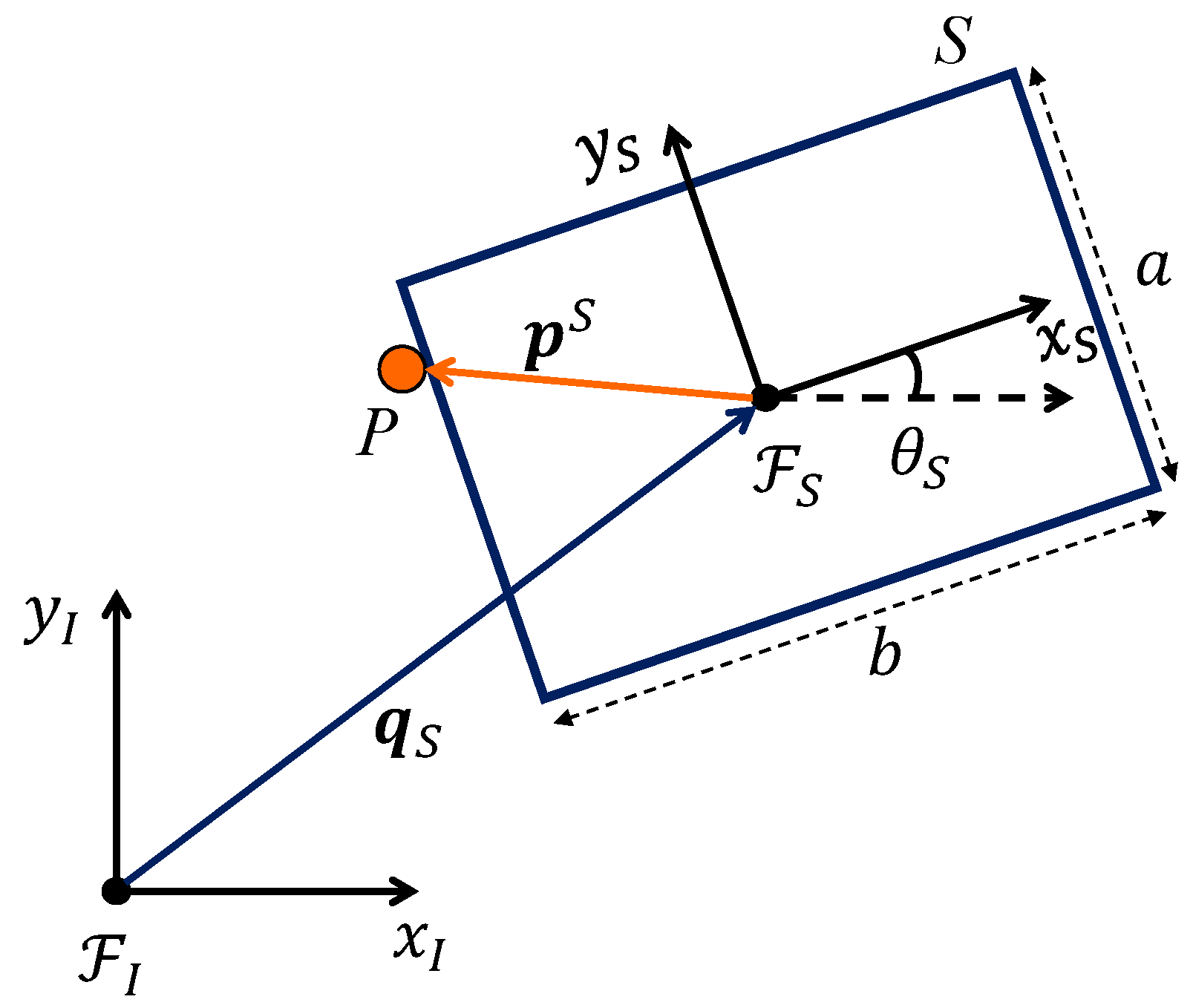
3.1. Dynamic Model

Referring to Figure 2, the pusher–slider system consists of a rigid object S, the slider, that can translate and rotate in a plane and whose configuration is described by a vector ${\mathit{q}}_S={\left[\begin{array}{ccc}{x}_s& y_s& \theta \end{array}\right]}^T$ with respect to an inertial reference frame ${\mathcal{F}}_I$. In the present study, the slider is a rectangular object, defined by its width a and its length b. The slider is moved by another rigid object P, the pusher, assuming that their interaction occurs through a single contact point. Its coordinates in the plane are expressed according to the position of the slider, i.e., ${\mathit{p}}^S={\left[\begin{array}{cc}{p}_x^S& p_y^S\end{array}\right]}^T$, with respect to the slider frame ${\mathcal{F}}_S$, centered in the center of friction of the slider (CF).

The following assumptions will be used to derive the equations of motion:

• The pusher and the slider move in the horizontal plane normal to the gravity vector and all forces lie in this plane.
• Pusher motion is slow enough that inertial forces are negligible compared to frictional forces (quasi-static assumption).
• The friction forces are governed by the Coulomb’s Law: the tangential force of friction during sliding lies along the opposite direction to the direction of motion, with magnitude proportional to the normal force.
• The friction coefficient between the slider and the support surface, ${\mu }_{SS}$, is uniform. It means that the CF is simply the projection of the center of mass (CM) in the plane.
• The pusher is assumed always be in contact with the slider in a point ${\mathit{p}}^S$.

By following the approach developed in the literature, in order to model the interaction between the pusher and the slider in terms of velocities, the construction of the so-called motion cone, introduced by Mason in [5], is required. By using the ellipsoidal approximation of the limit surface used to model the two-dimensional slippage as in [7], a mapping between the generalized friction forces and the slider twist is recovered. By evaluating the wrench at the contact point, this mapping is used to evaluate the boundaries of the motion cone, i.e., ${\mathit{v}}_l={\left[\begin{array}{cc}1& {\gamma }_l\end{array}\right]}^T$ and ${\mathit{v}}_r={\left[\begin{array}{cc}1& {\gamma }_r\end{array}\right]}^T$, where the explicit definition of the ${\gamma }_l$ and ${\gamma }_r$ coefficients can be found in [9]. According to the analogy between the friction cone and the motion cone, they play the same role for the tangential and normal components of the velocity as the friction coefficient for the tangential and normal force components, i.e., they are the ratio of the minimal tangential component (along the y axis) over the normal component (along the x axis), which generates a sliding. This representation allows us to determine if the velocity applied to the slider by the pusher, let it be ${\mathit{v}}_p^S={\left[\begin{array}{cc}{v}_{px}^S& v_{py}^S\end{array}\right]}^T$ with respect to ${\mathcal{F}}_S$, results in a sticking or a sliding behavior of the objects in contact. Indeed, if ${\mathit{v}}_p^S$ is inside the motion cone, the contact between slider and pusher results in a sticking mode and the velocity is fully transmitted to the slider; if ${\mathit{v}}_p^S$ exceeds one of the edges of the motion cone, only a part of it is transmitted to the slider and the remaining part determines a sliding of the pusher on the object, i.e., if ${\mathit{v}}_p^S$ exceeds ${\mathit{v}}_l$, a sliding left contact mode occurs, and if ${\mathit{v}}_p^S$ exceeds ${\mathit{v}}_r$, a sliding right takes place.

Depending on the contact modes $j=ST,SL,SR$, which correspond to sticking, sliding left and sliding right, respectively, the hybrid dynamics of the system under examination can be represented under the following constraints:

$$\dot{\mathit{x}}=\mathit{f}(\mathit{x},\mathit{u})=\left\{\begin{array}{cc}{\mathit{f}}_{ST}(\mathit{x},\mathit{u}),\hfill & \mathrm{if}{\gamma }_r\le v_{py}^S/v_{px}^S\le {\gamma }_l\hfill \\ {\mathit{f}}_{SL}(\mathit{x},\mathit{u}),\hfill & \mathrm{if}{v}_{py}^S/v_{px}^S>{\gamma }_l\hfill \\ {\mathit{f}}_{SR}(\mathit{x},\mathit{u}),\hfill & \mathrm{if}{v}_{py}^S/v_{px}^S<{\gamma }_r\hfill \end{array}\right.$$

(3)

where $\mathit{x}={\left[\begin{array}{cc}{\mathit{q}}_S^T& p_y^S\end{array}\right]}^T$ is the state of the system and $\mathit{u}={\left[\begin{array}{cc}{v}_{px}^S& v_{py}^S\end{array}\right]}^T$ is the control input represented by the normal and tangential pusher velocity, respectively, expressed in ${\mathcal{F}}_S$. An explicit formulation of ${\mathit{f}}_j(\mathit{x},\mathit{u})$ can be found in [9].

3.2. Control System Design

The role of the proposed feedback controller is to determine the best pusher velocity to counteract the displacement from the desired trajectory. The controller is based on the feedback of the state $\mathit{x}$, i.e., the slider pose that has to be measured by a visual tracker and the pusher position that is measured through the robot forward kinematics. To achieve the best performance, the maximum accuracy in system modeling is required, but this is really hard to obtain due to the difficulties in friction forces modeling. Therefore, the controller has to be robust enough to address the uncertainties of the model as well as the external disturbances. Moreover, the controller has to deal with the underactuation of the system and its hybrid nature, i.e., the constraints of the motion cone described in (3) have to be explicitly accounted for in the controller design. A Model Predictive Control (MPC) has proven to be the most suitable solution to satisfy all the requirements above.

In order to achieve a real-time control law, rather than considering the highly nonlinear dynamics in (3) in the control system design, its linearization about a given straight line is used, as proposed in [9]. Depending on the contact mode j, both the equations of motion and the constraints in (3) can be written in a matrix form as

$$\delta \dot{\mathit{x}}\left(t\right)={\mathit{A}}_j\left(t\right)\delta \mathit{x}\left(t\right)+{\mathit{B}}_j\left(t\right)\delta \mathit{u}\left(t\right),$$

(4)

$${\mathit{E}}_j\left(t\right)\delta \mathit{x}\left(t\right)+{\mathit{D}}_j^T\left(t\right)\delta \mathit{u}\left(t\right)\le {\mathit{g}}_j^T\left(t\right),$$

(5)

respectively, where $\delta \mathit{x}\left(t\right)$ and $\delta \mathit{u}\left(t\right)$ represent the perturbation about the equilibrium state $\overline{\mathit{x}}$ and about the nominal input $\overline{\mathit{u}}$. The explicit expression of matrices in (4) and (5) can be found in [9].

Consider the linearized system in (4) and the constraints expressed as linear inequalities in (5). Using the forward Euler integration method, the resulting equations in discrete time, depending on the contact mode, are:

$$\delta \mathit{x}(k+1)=(\mathit{I}+T_s{\mathit{A}}_j\left(k\right))\delta \mathit{x}\left(k\right)+T_s{\mathit{B}}_j\left(k\right)\delta \mathit{u}\left(k\right)$$

(6)

$${\mathit{E}}_j\left(k\right)\delta \mathit{x}\left(k\right)+{\mathit{D}}_j^T\left(k\right)\delta \mathit{u}\left(k\right)\le {\mathit{g}}_j^T\left(k\right),$$

(7)

where k denotes the time at which the equations are evaluated and $T_s$ is the sampling time. The controller design is developed by using (6) and (7), as described hereafter.

Let H be the finite length of the prediction horizon, which is assumed to be the same as the control horizon. The objective of the controller is to resolve the following optimization problem:

$$\begin{array}{c}\hfill \underset{\delta {\mathit{x}}_n,\delta {\mathit{u}}_n}{min}\mathit{J}(\delta \mathit{x},\delta \mathit{u})=\delta {\mathit{x}}_H^T{\mathit{W}}_H\delta {\mathit{x}}_H+\sum _{n=0}^{H-2}\delta {\mathit{x}}_{n+1}^T\mathit{W}\delta {\mathit{x}}_{n+1}+\sum _{n=0}^{H-1}\delta {\mathit{u}}_n^T\mathit{R}\delta {\mathit{u}}_n\\ \hfill \mathrm{s}.\mathrm{t}.\left\{\begin{array}{c}\mathrm{if}n=0\left\{\begin{array}{cc}& \delta {\mathit{x}}_1=\delta {\mathit{x}}_0-T_s\left(f({\overline{\mathit{x}}}_0,{\overline{\mathit{u}}}_0)-{\overline{\mathit{B}}}_{j0}{\mathit{u}}_0\right)\hfill \\ & {\overline{\mathit{D}}}_{j0}^T{\overline{\mathit{u}}}_0\le {\overline{\mathit{g}}}_{j0}^T\hfill \end{array}\right.\hfill \\ \\ \mathrm{if}n>0\left\{\begin{array}{cc}& \delta {\mathit{x}}_{n+1}=\left(\mathit{I}+T_s{\mathit{A}}_{jn}\right)\delta {\mathit{x}}_n+T_s{\mathit{B}}_{jn}\delta {\mathit{u}}_n\hfill \\ & {\mathit{E}}_{jn}\delta {\mathit{x}}_n+{\mathit{D}}_{jn}^T\delta {\mathit{u}}_n\le {\mathit{g}}_{jn}^T\hfill \end{array}\right.\hfill \\ \\ u_{xm}\le u_x\le u_{xM}\hfill \\ u_{ym}\le u_y\le u_{yM}\hfill \\ -\lambda \frac{b}{2}\le p_y^S\le \lambda \frac{b}{2}\hfill \end{array}\right.\end{array}$$

(8)

where n denotes the step along the prediction horizon and the subscript $n+1$ stands for $t_{n+1}$. $\mathit{W}$ is the weight matrix for the error state, while $\mathit{R}$ weighs the control input. At the final step, $n=H$, the error state is weighted with a matrix ${\mathit{W}}_H$ used to approach a zero steady-state error. Note that for $n=0$ a different formulation of constraints, arising from nonlinear equations, is used so that a greater fidelity to the model is achieved. In fact, thanks to the knowledge of ${\mathit{x}}_0$ (note that it is not an optimization variable because it corresponds to the measurement at time $t_0$ of the prediction horizon), the Equation (3) reduced automatically to a linear form for both the dynamics and the constraints. Moreover, $u_{xm},u_{ym}$ and $u_{xM},u_{yM}$ represent the minimum and the maximum normal and tangential pusher velocities allowed, respectively, and a last constraint is used to force the pusher not to slide over $\lambda \frac{b}{2}$ of the sliding object, where $\lambda$ is a scalar safety factor.

By following the approach in [9], in order to address the hybrid nature of the system without increasing the computational complexity of the problem, the sub-optimal family of modes approach has been adopted in the controller design. It consists in selecting $\eta$ of the $3^H$ possible sequences along the prediction horizon, so that a wide range of system behaviors is covered and only $\eta$ constrained quadratic optimization problems have to be solved. Note that, the choice of such parameters is critical: a too-high number of sequences results in a high computational complexity while a too-low number may not be sufficient to cover the significant dynamic behaviour of the system. Considering that the MPC is such that only the first computed input is used, the following family of modes has been chosen for the controller design:

$$\begin{array}{cc}\hfill \mathcal{M}=\{& (S{T}_1,\cdots ,S{T}_H),\hfill \\ & (S{L}_1,\cdots ,S{L}_{H_m},S{T}_{H_{m+1}},\cdots ,S{T}_H),\hfill \\ & (S{R}_1,\cdots ,S{R}_{H_m},S{T}_{H_{m+1}},\cdots ,S{T}_H)\},\hfill \end{array}$$

(9)

where $H_m$ represents the number of steps for which the initial contact mode is maintained and $S{T}_j,S{L}_j,S{R}_j$ represent the sticking, sliding left, and sliding right modality at step $j=1,\cdots ,H$, respectively. This choice not only fits well to cover most of the dynamic behaviors between the slider and the pusher, but also allows us to drastically reduce the computational cost of the problem under examination. In fact, in this way, the controller has to resolve only three ($\eta =3$) QP problems as formulated in (8), one for each sequence of the family. Subsequently, the best sequence of the contact mode corresponds to the one for which the optimization problem gave the minimum value of the cost function.

In view of the hybrid nature of the pusher–slider system, an aspect that was overlooked by the authors of [9] proposing the control strategy above is the control effort required to switch from one mode to another. Specifically, if the switches occur at high frequency, an undesirable phenomenon of chattering may occur. A way to reduce as much as possible the oscillations consists in making the switches happen only when strictly necessary. A design parameter helpful to regulate them is $H_m$, which can be selected in the range $\left[1,H\right]$. Suppose that the controller is in the sticking mode and that a small angular error affects the system state. If $H_m$ is too low, the controller will consider optimum to switch between sticking and sliding mode to recover the error as soon as possible. The continuous switching between the two modes results in an oscillating control signal. To avoid this behavior, $H_m$ has to be set to a value not too low. Note that, even the opposite extreme is to be avoided, otherwise the system may be too slow to recover from errors and disturbances. On the other hand, by analyzing the cost functions trend of the three contact modes, it was observed that their values differ for a small threshold, let it be $ϵ$, when small deviations from the nominal trajectory occur. Therefore, in these situations, the controller switches from one mode to another unnecessarily, causing continuous oscillations in the control signal. To avoid it, a new countermeasure has been adopted here: given $ϵ$, at each iteration, after solving the three QP problems, the mode chosen at the previous step is privileged by subtracting the threshold $ϵ$ to its new minimum, as shown in Algorithm 1, where $inde{x}_{k-1}$ represents the mode j chosen at the previous step.

Algorithm 1: Chattering avoidance.

Data: $\delta {\mathit{x}}_k,inde{x}_{k-1},ϵ$ $mi{n}_{STk}\leftarrow \mathrm{solve}\mathrm{QP}\mathrm{for}\mathrm{sticking}\mathrm{mode}$ $mi{n}_{SLk}\leftarrow \mathrm{solve}\mathrm{QP}\mathrm{for}\mathrm{sliding}\mathrm{left}\mathrm{mode}$ $mi{n}_{SRk}\leftarrow \mathrm{solve}\mathrm{QP}\mathrm{for}\mathrm{sliding}\mathrm{right}\mathrm{mode}$ $so{l}_k\leftarrow \left[mi{n}_{STk},mi{n}_{SLk},mi{n}_{SRk}\right]$ $sol\left(inde{x}_{k-1}\right)\leftarrow sol\left(inde{x}_{k-1}\right)-ϵ$ $mod{e}_{opt}\leftarrow min\left(so{l}_k\right)$

3.3. Explicit Delay Compensation

Although using efficient tools to solve the optimization problems arising from the family of modes approach allows us to achieve a real-time controller, with a digital implementation other sources of latency may cause delays in a feedback controller. For example, in many cases, the systems to be controlled have dynamics characterized by delays not negligible, so that an input u is actuated with a delay d by the system. This is the typical case of robot control interfaces, where a reference position, or velocity, or torque is checked and buffered or filtered before being actuated. Moreover, the perception pipeline could also be affected by communication delays, especially if the computing hardware running the neural networks is different from the computing unit running the controller. In this case, in view of (6) and assuming that all system inputs are subject to the same delay, the delayed model can be represented as

$$\delta \mathit{x}(k+1)={\mathit{A}}_k\delta \mathit{x}\left(k\right)+{\mathit{B}}_k\delta \mathit{u}(k-d),$$

(10)

where ${\mathit{A}}_k=\mathit{I}+T_s{\mathit{A}}_j\left(k\right)$, ${\mathit{B}}_k=T_s{\mathit{B}}_j\left(k\right)$ and the delay is equal to d sampling periods. To address the latency of the system, an explicit delay compensation, based on an approach that was first formulated in [34] for an interior-point optimization algorithm, is preferred to the implicit one, so that the representation order of the system does not depend on the number of delayed samples d.

Equation (10) reveals that, due to the input delay, the state at time k does not depend on the current input $\delta \mathit{u}\left(k\right)$ but only on the previous input obtained at time $k-d-1$. In other words, the effect of the input at time k affects the state only d samples later.

By observing that the state $\delta \mathit{x}(k+d|k)$ can be recovered recursively from (10), it results in

$$\delta \mathit{x}(k+d|k)={\mathit{A}}_k^d\delta \mathit{x}\left(k\right)+\sum _{\nu =1}^d{\mathit{A}}_k^{\nu -1}{\mathit{B}}_k\delta \mathit{u}(k-\nu ).$$

(11)

By modeling the delay as a FIFO (First-In-First-Out) buffer of fixed length d, according to (11), the MPC design can still be based on a delay-free system, because the delay compensation is explicitly addressed. Naturally, at time k, it is necessary to predict the state in which the system will obtain d samples later, applying to the plant model the control inputs recorded in the buffer delay.

Figure 3 shows the system architecture arising from this approach. Given the measured state $\mathit{x}\left(k\right)$ and the nominal trajectory evaluated d samples later, i.e., $\overline{\mathit{x}}(k+d|k)$, the predictor has to simulate the dynamics of the pusher–slider system along the delay buffer. By swiping the buffer from the last element to the first one, firstly the predictor has to evaluate the motion cone constraints and then has to simulate the system dynamics. Finally, the predicted state at time k, i.e., $\widehat{\mathit{x}}(k+d|k)$, is given to the controller to evaluate the next perturbed input controller $\delta \mathit{u}\left(k\right)$, that will enter the buffer. This delay compensation strategy was essential to obtain a good behavior of the closed loop system running at a sampling time compatible with the actual update rate of the visual tracker, rather than using a fictitiously high sample rate for the control computation as in [9].

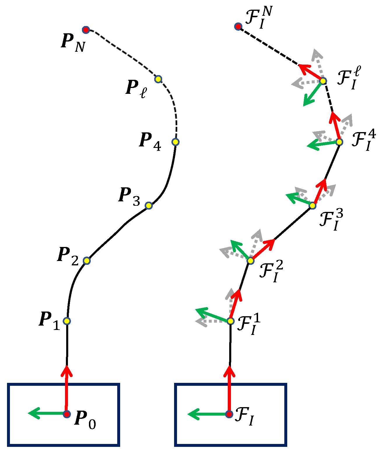
3.4. Trajectory Generation

Due to the linearization of the pusher–slider system model about a straight line, the tracking of more complex trajectories including curves might fail. Still inspired by [9], a novel strategy is here proposed for the generation of the trajectory characterized by paths with different shapes, which allows us to re-use the controller designed for tracking the straight line. The novel strategy conveniently switches the inertial reference frame ${\mathcal{F}}_I$ during the execution of a complex trajectory in order to deceive the controller to think of following the straight-line trajectory, while allowing separation of translation movements from rotational ones.

Let $P_1,\cdots ,P_N$ be a set of points, belonging to a feasible path in the plane $xy$ and ${\mathit{p}}_{\ell }={\left[\begin{array}{cc}{p}_{x_{\ell }}& p_{y_{\ell }}\end{array}\right]}^T$ is the vector of coordinates of the point $P_{\ell }$ expressed in the inertial frame ${\mathcal{F}}_I$, with $\ell =1,\cdots ,N$. Given the initial position of the slider expressed by the point $P_0$, the planned path is approximated by N segments connecting these points, i.e., the set of segments from $P_{\ell }$ to $P_{\ell +1}$, with $\ell =0,\cdots ,N-1$.

The desired 2D poses of the slider expressed in ${\mathcal{F}}_I$, corresponding to each target point, are recovered by splitting the translations from the rotations, so that each target pose defines a pure translation or a pure rotation. Let $\mathit{X}$ be the matrix grouping all the desired poses, obtained from the split. Without loss of generality, suppose the first target point $P_1$ lies on the x axis of ${\mathcal{F}}_I$, i.e., $p_{y_1}=0$. It follows that the first segment is a straight line that does not require a rotation. The matrix $\mathit{X}$ is defined as follows:

$$\mathit{X}=\left[\begin{array}{ccc}{p}_{x_1}& p_{y_1}& {\Theta }_0\\ p_{x_1}& p_{y_1}& {\Theta }_1\\ ⋮& ⋮& ⋮\\ p_{x_{\ell }}& p_{y_{\ell }}& {\Theta }_{\ell -1}\\ p_{x_{\ell }}& p_{y_{\ell }}& {\Theta }_{\ell }\\ ⋮& ⋮& ⋮\\ p_{x_N}& p_{y_N}& {\Theta }_{N-1}\end{array}\right],$$

(12)

with ${\Theta }_0=0$ and ${\Theta }_{\ell }={\Theta }_{\ell -1}+\mathrm{atan}2\left(p_{y_{\ell +1}}-p_{y_{\ell }},p_{x_{\ell +1}}-p_{x_{\ell }}\right)$ for $\ell =1,\cdots ,N-1$. It follows that the last desired trajectory is a pure translation.

Note that, even if the trajectory is defined through a sequence of straight lines, some of these may require a rotation of the slider, i.e., ${\Theta }_{\ell }\ne 0$. In these cases, the pusher–slider system would move too far away from the trajectory around which it is linearized, so that its real behavior would not be faithful to the linearized form used in the control design anymore. To avoid this, the frame ${\mathcal{F}}_I$ has to be updated at the end of each segment, let it be ${\mathcal{F}}_I^{\ell }$, making sure that its axis $x_I^{\ell }$ points from the actual position of the slider to the target one, as shown in Figure 4. Consequently, the slider pose has to be expressed in the updated frame ${\mathcal{F}}_I^{\ell }$. In this way, it is ensured that the system never deviates too far from the nominal trajectory used for its linearization and the controller is tricked into thinking that the overall trajectory is a straight line.

In turn, this means that at each time instant t the new nominal state trajectory in correspondence of a pure translation is updated as

$$\overline{\mathit{x}}\left(t\right)=\left[\begin{array}{c}{\mathit{p}}_{\ell }^{\ell }+\frac{{\mathit{p}}_{\ell +1}^{\ell }-{\mathit{p}}_{\ell }^{\ell }}{\parallel {\mathit{p}}_{\ell +1}^{\ell }-{\mathit{p}}_{\ell }^{\ell }\parallel }{v}_{px}^S\left(t-t_{0_{\ell }}\right)\\ 0\\ 0\end{array}\right],t\in [t_{0_{\ell }},t_{f_{\ell }}],$$

(13)

where $t_{0_{\ell }}$ is the initial time of each partial trajectory, $t_{f_{\ell }}$ is the duration of the segment, evaluated as $\frac{\parallel {\mathit{p}}_{\ell +1}^{\ell }-{\mathit{p}}_{\ell }^{\ell }\parallel }{v_{px}^S}$, and, ${\mathit{p}}_{\ell }^{\ell }$ represents the point ${\mathit{p}}_{\ell }$ expressed in ${\mathcal{F}}_I^{\ell }$. Note that, due to the frame updating, it always results ${\overline{y}}_s^{\ell }=0$. As shown in Figure 4, this approach is such that the system may not be attached to the nominal trajectory expressed in the updated frame ${\mathcal{F}}_I^{\ell }$, due to a higher or lower angle error. As this error grows, the effort required to the control grows. In order to always keep a moderate control, it is possible to add an angular smooth reference in correspondence to the pure rotation step, i.e.,

$$\overline{\mathit{x}}\left(t\right)=\left[\begin{array}{c}0\\ 0\\ {\Theta }_{\ell }^{\ell }+\frac{{\Theta }_{\ell +1}^{\ell }-{\Theta }_{\ell }^{\ell }}{\parallel {\Theta }_{\ell +1}^{\ell }-{\Theta }_{\ell }^{\ell }\parallel }\alpha \left(t-t_{0_{\ell }}\right)\\ 0\end{array}\right].$$

(14)

where ${\Theta }_{\ell }^{\ell }$ is the angle ${\Theta }_{\ell }$ expressed in ${\mathcal{F}}_I^{\ell }$, $\alpha$ is the angular velocity of the reference, $t_{0_{\ell }}$ is the initial time of the partial trajectory, and, $t_{f_{\ell }}$ is the duration of the rotation, evaluated as $\frac{|{\Theta }_{\ell +1}^{\ell }-{\Theta }_{\ell }^{\ell }|}{\alpha }$.

Note that, in particular, since ${\Theta }_{\ell }^{\ell }$ in (14) and ${\mathit{p}}_{\ell }^{\ell }$ in (13) are both expressed in the updated frame ${\mathcal{F}}_I^{\ell }$, it results ${\Theta }_{\ell }^{\ell }=0$ and ${\mathit{p}}_{\ell }^{\ell }=\mathit{0}$.

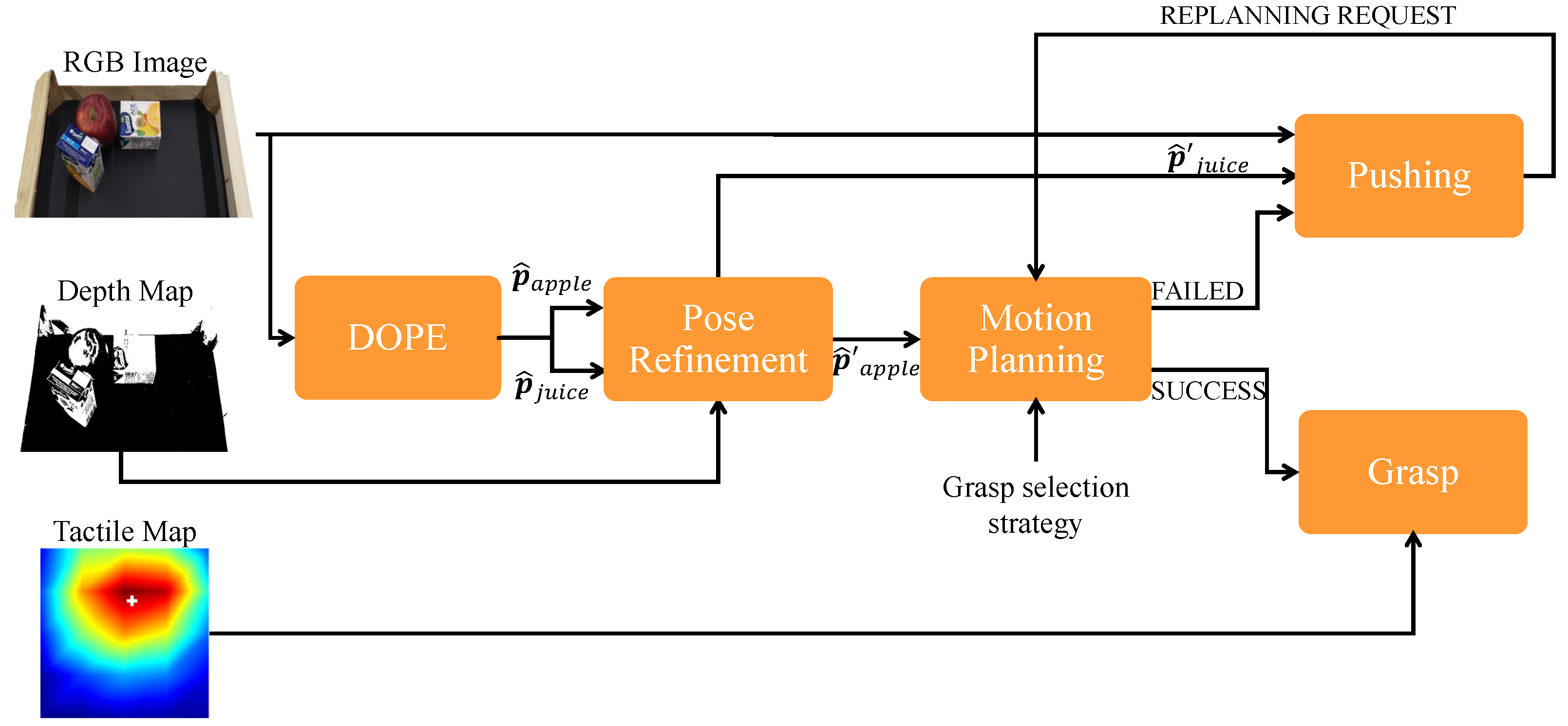
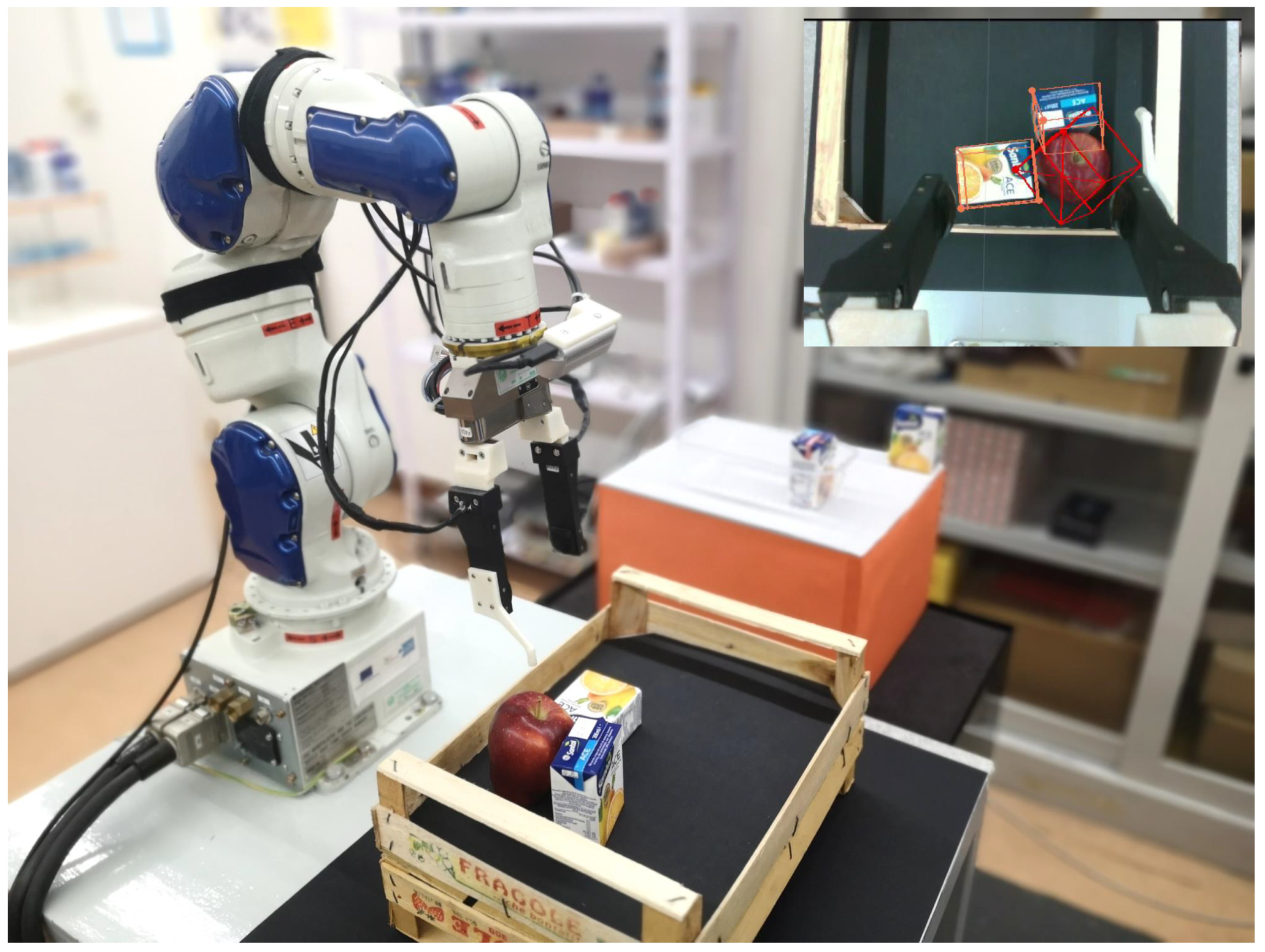
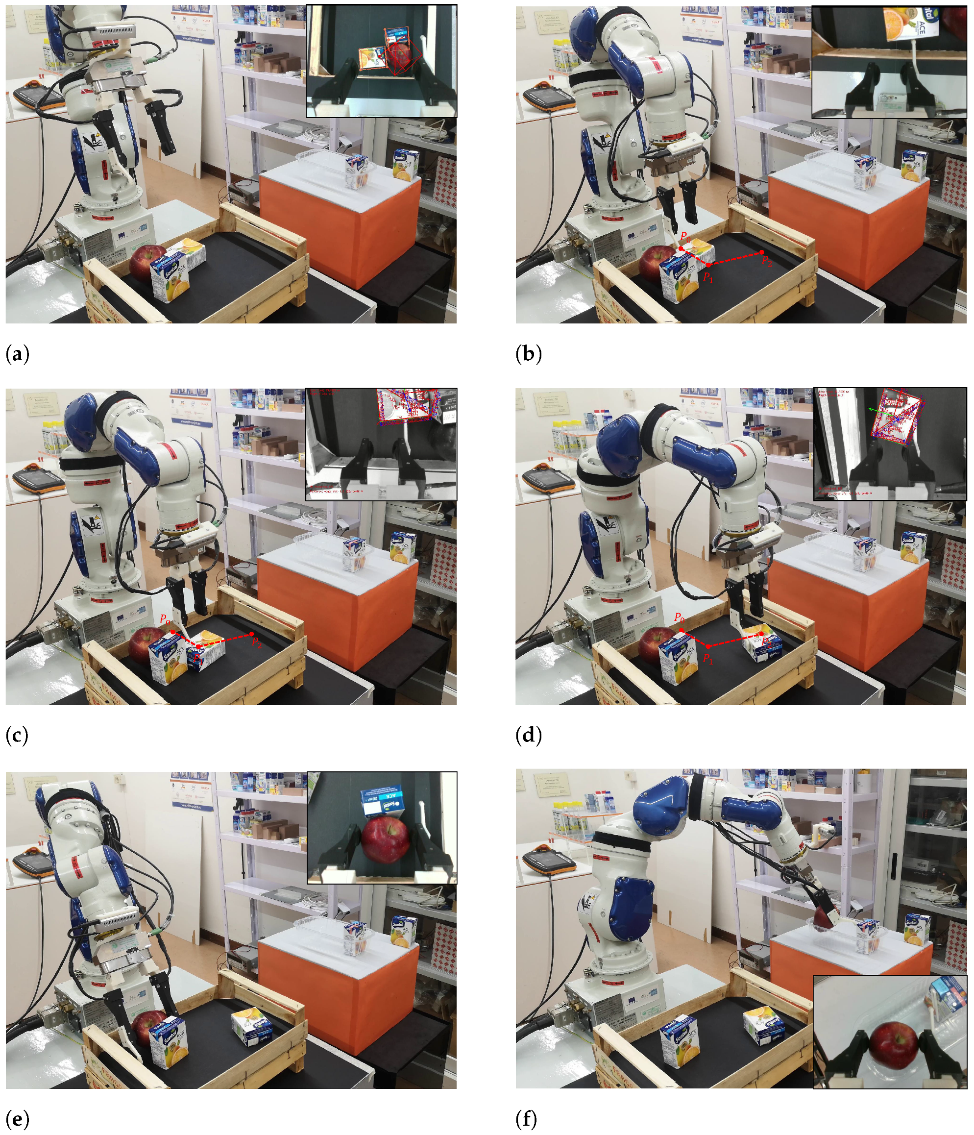
4. Pipeline for Pick-and-Place of Fruits

The overall pick-and-place pipeline, already developed in [10], is here extended with the non-prehensile manipulation ability of the pushing as explained hereafter. Figure 5 shows how it works in a specific context, in which the goal is to pick the target object, a red apple, in a cluttered scene. The pipeline starts with the perception step, which makes the system aware of its surroundings, by determining the position and orientation of the objects in the space through DOPE, and by refining the resulting estimated poses with the pose refinement algorithm as described in Section 2.2. Given the refined pose of the target object, ${\widehat{p}}_{apple}^{\prime }$, a motion planning module, described in [10], plans to pick the object. It takes in input a grasp pose chosen by the grasp selection strategy described in Section 4.1. If the motion planning is successful in finding a collision-free path to pick and place the red apple, a grasp force controller, as described in Section 4.1, is used to grasp the object with the minimum force necessary to lift it. Otherwise, a pushing action is requested to the pushing module to facilitate the grasp maneuver. The pushing module, described in Section 3, takes in input the pose of the selected obstacle in the scene, let it be ${\widehat{p}}_{juice}^{\prime }$, and pushes it to a target location. Then, planning trials and pushing actions follow in an iterative way until the motion planning is successful.

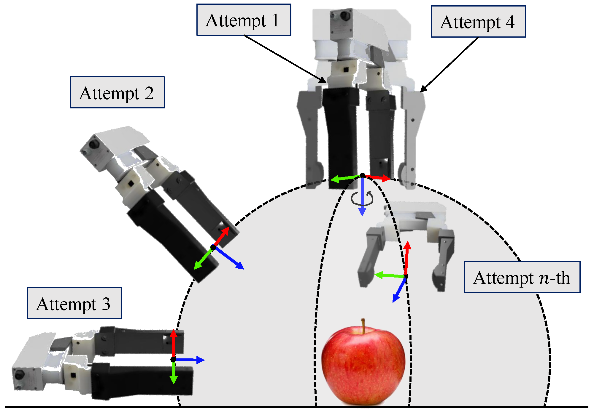
4.1. Grasp Force Control and Grasp Selection Strategy

Even if the described grasping pipeline is successful owing to the accurate pose estimation and to the non-prehensile helping maneuver, the actual handling of fruits and vegetables is a non-trivial issue. This is because, even considering objects of the same type (e.g., two apples), they have different physical properties such as weight, shape, friction, and deformability. Moreover, depending on the robot’s acceleration, the handled object is also subject to inertial forces, thus an open loop grasp force control might not be robust enough to avoid object slipping while limiting the object deformation at the same time.

To tackle this issue and enhance the manipulation robustness, we adopt the slipping control strategy proposed in [30,31] based on the force/tactile feedback provided by the SunTouch sensors [29]. The algorithm aims at automatically regulating the grasp force to the minimum required force that avoids slippage.

The grasp force control algorithm is briefly described in the following, but more details are available in [31].

Similarly to the pusher modeling, the control strategy is a model-based algorithm that exploits the LS theory which is an extension of the classical Coulomb friction to roto-translational motions. This way the model is aware not only of the translational load but also of the rotational ones. The resulting grasping force takes into account both contributions which are strongly coupled, in fact, the grasp force that avoids slippage is usually much higher in case torsional loads are applied to the grasped object.

The grasp force $f_n$ is computed by the grasp controller as the sum of two contributions, i.e.,

$$f_n=f_{n_s}+f_{n_d}.$$

(15)

$f_{n_s}$ is the so-called static contribution and is computed by using the LS theory and the force and torque measurements at the fingertips. This contribution allows a safe grasp of objects with unknown weight and grasp location in quasi-static conditions. When the load varies (e.g., during the lift and the transport) such a contribution might not be enough and a dynamic model should be taken into account. To tackle this issue the dynamic contribution$f_{n_d}$ is added to the control law. This control action is based on the slipping velocity estimated by a nonlinear observer thanks to a planar slider slippage model [31]. Specifically, $f_{n_d}$ is a linear control action that aims to regulate the estimated slippage velocity to zero.

A robotic solution for fruit picking able to operate independently in different situations should have the ability to automatically select the grasping pose depending on the obstacles in the scene. To increase the chances to pick the target object although the obstacles in the scene, the grasp selection strategy proposed in [10] is adopted.

The strategy allows to define a set of pre-grasp poses for the end effector frame, such that its origin is located on the surface of a sphere whose center is positioned in the refined position of the target object, and its approach vector (z-axis) points towards the center of said sphere. Figure 6 shows some examples of grasp poses defined following the aforementioned grasp selection strategy. A complete description of the method can be found in [10].

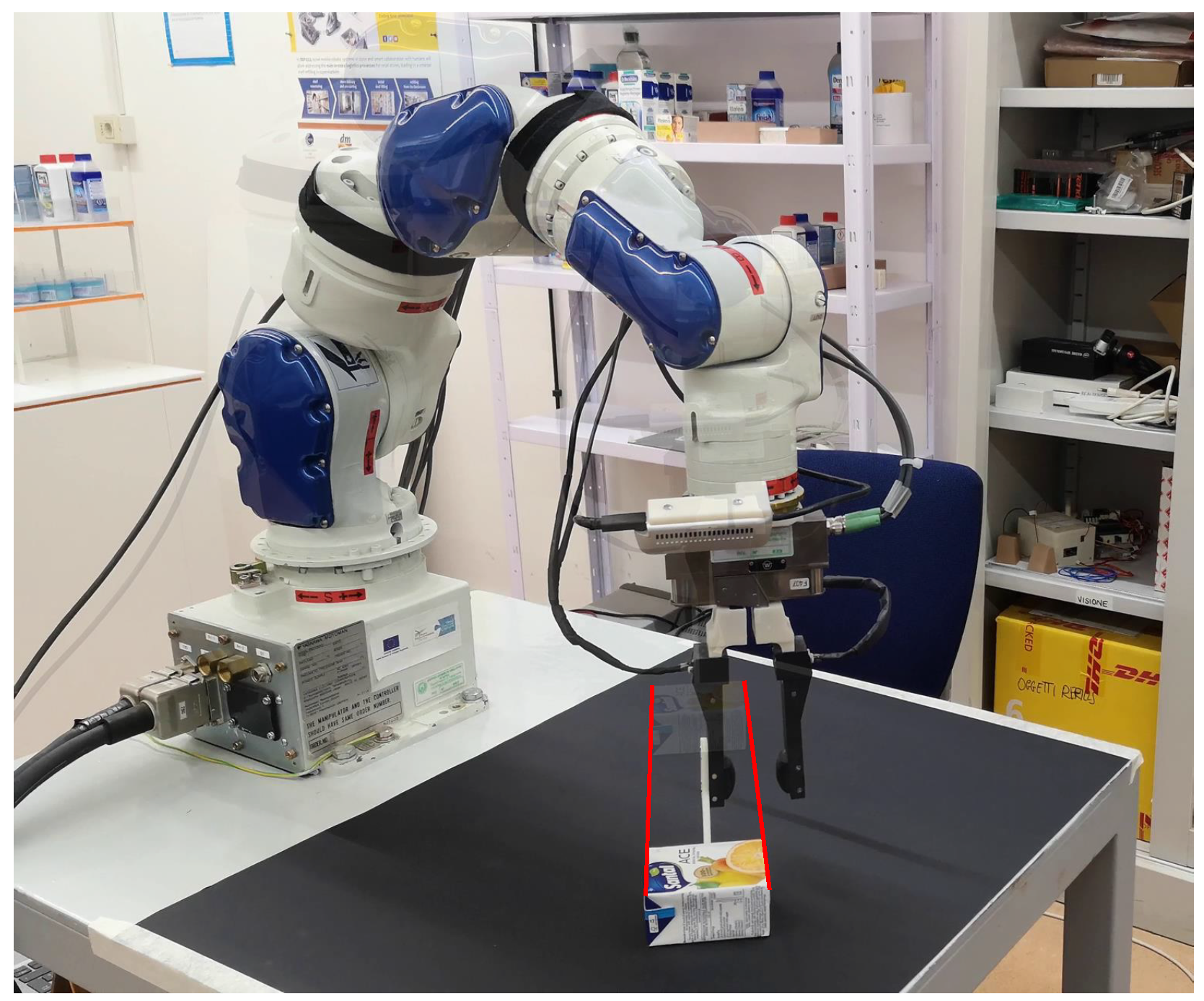
5. Experimental Results

The experiments are carried out on a seven-axis robot Yaskawa Motoman SIA5F equipped with a WSG32 gripper by Weiss Robotics, sensorized with the SUNTouch force/tactile fingers [29] and a RealSense Depth Camera D435i mounted on the robot gripper. The right finger of the robot is linked to a pushing extension suitably designed and realized in ABS plastic; its extremity is used by the robot to perform the pushing maneuver. The optimization problem described in (8) is solved using a state-of-the-art solver for mathematical programming, the Gurobi Optimizer [35], the communication with the robot takes place through the Robot Operating System (ROS) and a 3D model-based tracking system is realized through the platform ViSP [36] to measure the 2D pose of the slider in order to realize the feedback control law.

Table 4. Parameters of the dynamic model and of the controller.

Dynamic model parameters
a	$0.062\mathrm{m}$
b	$0.082\mathrm{m}$
m	$0.287\mathrm{k}\mathrm{g}$
${\mu }_{SS}$	$0.32$
${\mu }_{SP}$	$0.19$
Controller parameters
$T_s$	$0.050\mathrm{s}$
d	3
H	20
$H_m$	3
$ϵ$	$0.001$
$u_{xm}$	$0.001\mathrm{m}/\mathrm{s}$
$u_{xM}$	$0.02\mathrm{m}/\mathrm{s}$
$u_{ym}$	$-0.05\mathrm{m}/\mathrm{s}$
$u_{yM}$	$0.05\mathrm{m}/\mathrm{s}$
$\lambda$	$0.75$
$\overline{\mathit{u}}$	${\left[\begin{array}{cc}0.005& 0\end{array}\right]}^T\mathrm{m}/\mathrm{s}$
$\mathit{W}$	$10\mathrm{diag}\left(\left[1,1,0.005,0.01\right]\right)$
${\mathit{W}}_H$	$200\mathrm{diag}\left(\left[3,3,0.03,0\right]\right)$
$\mathit{R}$	$10\mathrm{diag}\left(\left[1,1\right]\right)$

reports the model and controller parameters used in the experiments described in the following.

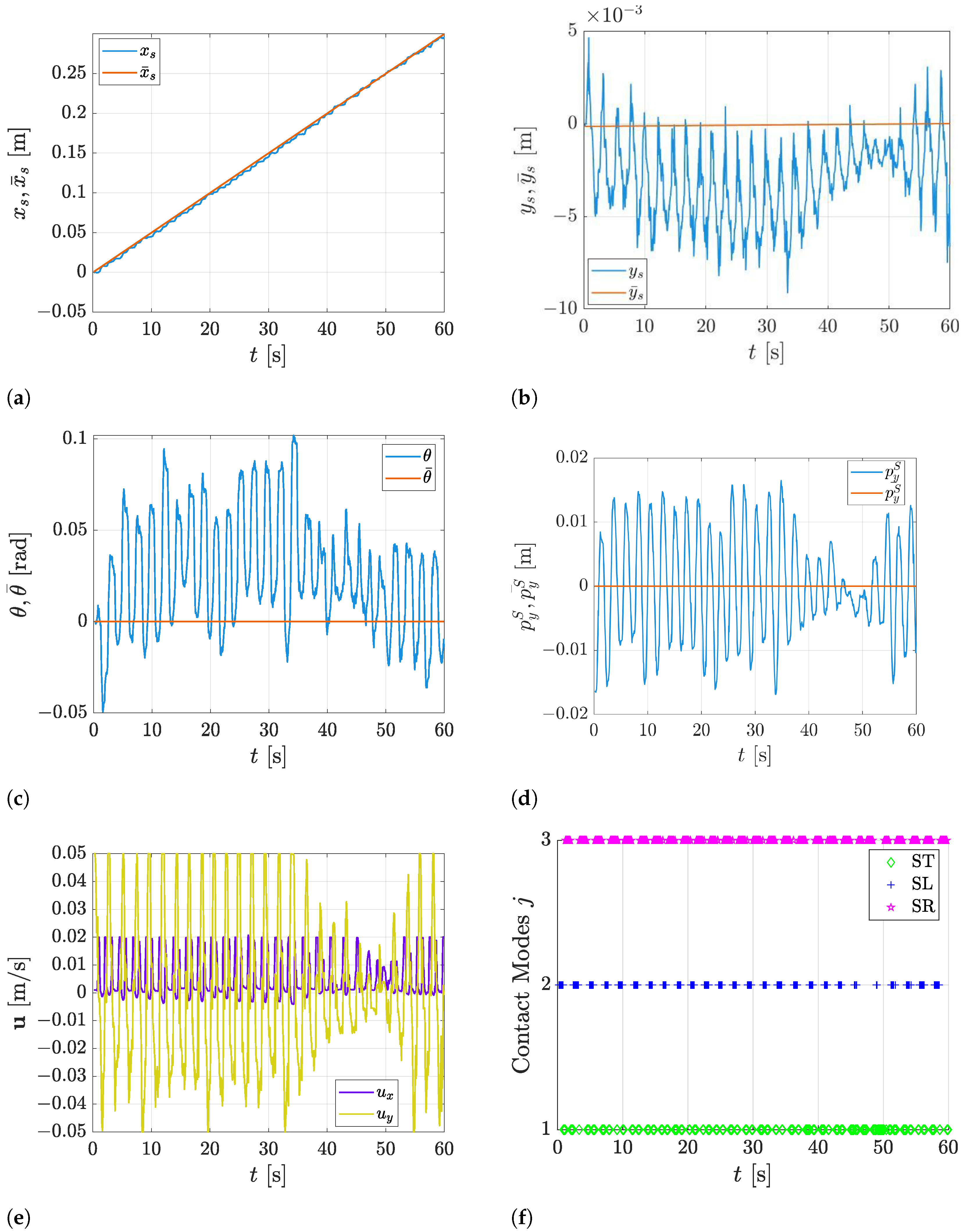
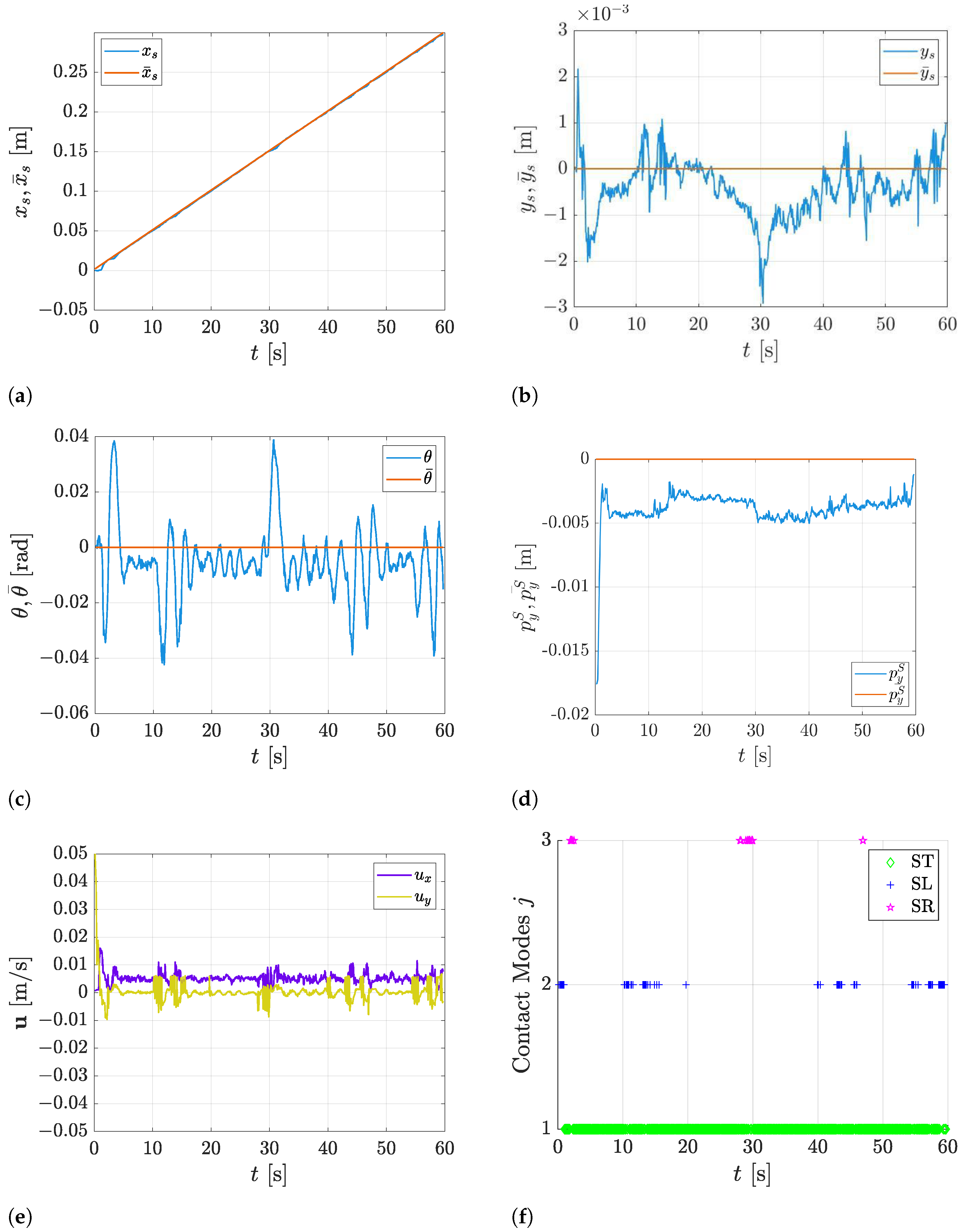
5.1. Comparison with the State-of-the-Art Approaches

To highlight the need of a feedback control, a first open-loop experiment was conducted. The proposed goal consists in pushing the slider for $0.3\mathrm{m}$ following a straight line with a nominal velocity $\overline{\mathit{u}}={\left[\begin{array}{cc}0.005& 0\end{array}\right]}^T\mathrm{m}/\mathrm{s}$. Figure 7 shows the experimental setup. As shown in Figure 8, even if the system has an almost zero initial error, the state diverges. This motivates the adoption of a feedback control.

The first closed-loop experiment has been conducted by using the state-of-the-art robotic pushing proposed by [9] without our improvements, here named STD-MPC (Standard MPC). It means that the chattering avoidance and the delay compensation strategies have not been used in the controller design, thus setting $d=0$, $H_m=1$, and $ϵ=0$ in Table 4. The desired trajectory has been generated as described in Section 3.4. Since straight-line tracking is required, only one point is used, i.e., $P_1=\left[\begin{array}{cc}0.30& 0\end{array}\right]\mathrm{m}$. Figure 9 shows the experimental results. It is evident how both the state and the control variables are affected by continuous high frequency oscillations caused by the delay that affects the digital implementation of the controller, given the large sampling time allowed by the perception module.

Therefore, we repeated the same experiment by adding the first of our contributions, namely, the delay compensation strategy explained in Section 3.3 to counteract this undesirable effect. The resulting controller is here named DC-MPC (Delay Compensation MPC). Figure 10d shows a great reduction of the oscillations in the evolution of both the state and the control signal. However, Figure 10e,f still highlight an unnecessary switching between the contact modes, considering that the tracking of a simple straight line is required. In order to reduce as much as possible the oscillations, as explained at the end of Section 3.2, the chattering avoidance strategy has been added in a third experiment, in which the proposed MPC is adopted. The choice of the parameters $d,H_m$, and $ϵ$ used for our improvements can be found in Table 4.

The experiment was carried out first in simulation in a Matlab environment, simulating also the measurement noise, and then on the real robot as Figure 11a–d illustrate the state evolution of the simulated closed-loop system, while Figure 11e shows the control signals $\mathit{u}$ applied to the simulated plant and Figure 11f shows the contact mode chosen at each step. The same order of figures is adopted in Figure 12 to show the results of the real experiment.

As expected, the real behavior of the system slightly deviates from the simulated one. This is unavoidable, due to the model uncertainties and the assumptions made on the plant. In particular, the non-uniform friction distribution of the contact surface in a real setting is certainly one of the main causes of the mismatch between simulation and reality.

Concerning the experimental results, the plots in Figure 12 show how the system is able to follow the reference signals achieving a steady-state error in the order of millimeters. Note that the slider is positioned by hand with an initial error on $p_y^S$. This justifies the choice of the controller to adopt the sliding contact mode right away so that the error can be recovered. Then, the sticking mode is preferred all the time, as expected since the tracking of a straight line is required. The results clearly demonstrate that no high frequency oscillation affects the state variable or the control variable, which saturates only at the initial time instant due to the initial error of almost $2$cm on the pusher position.

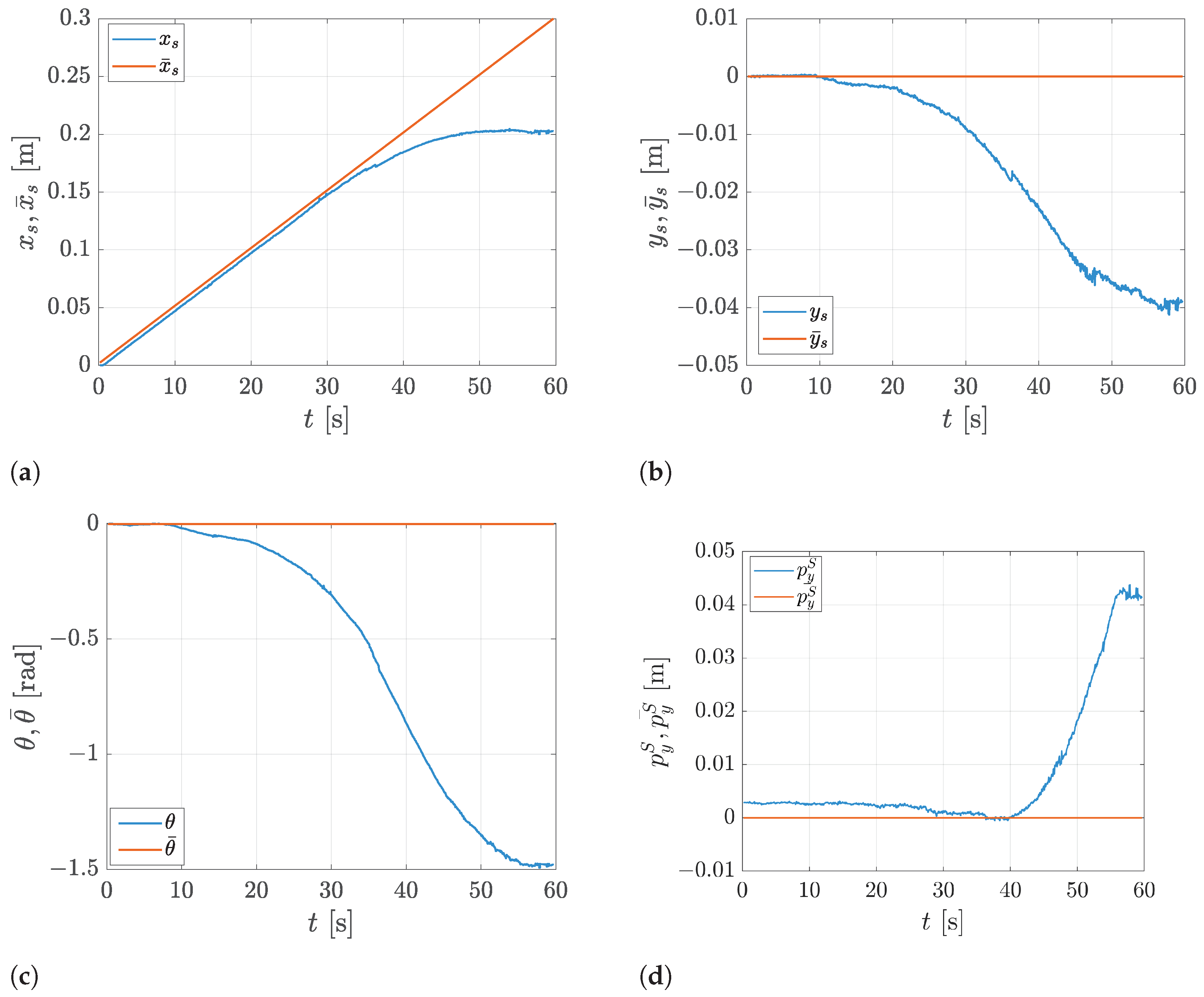
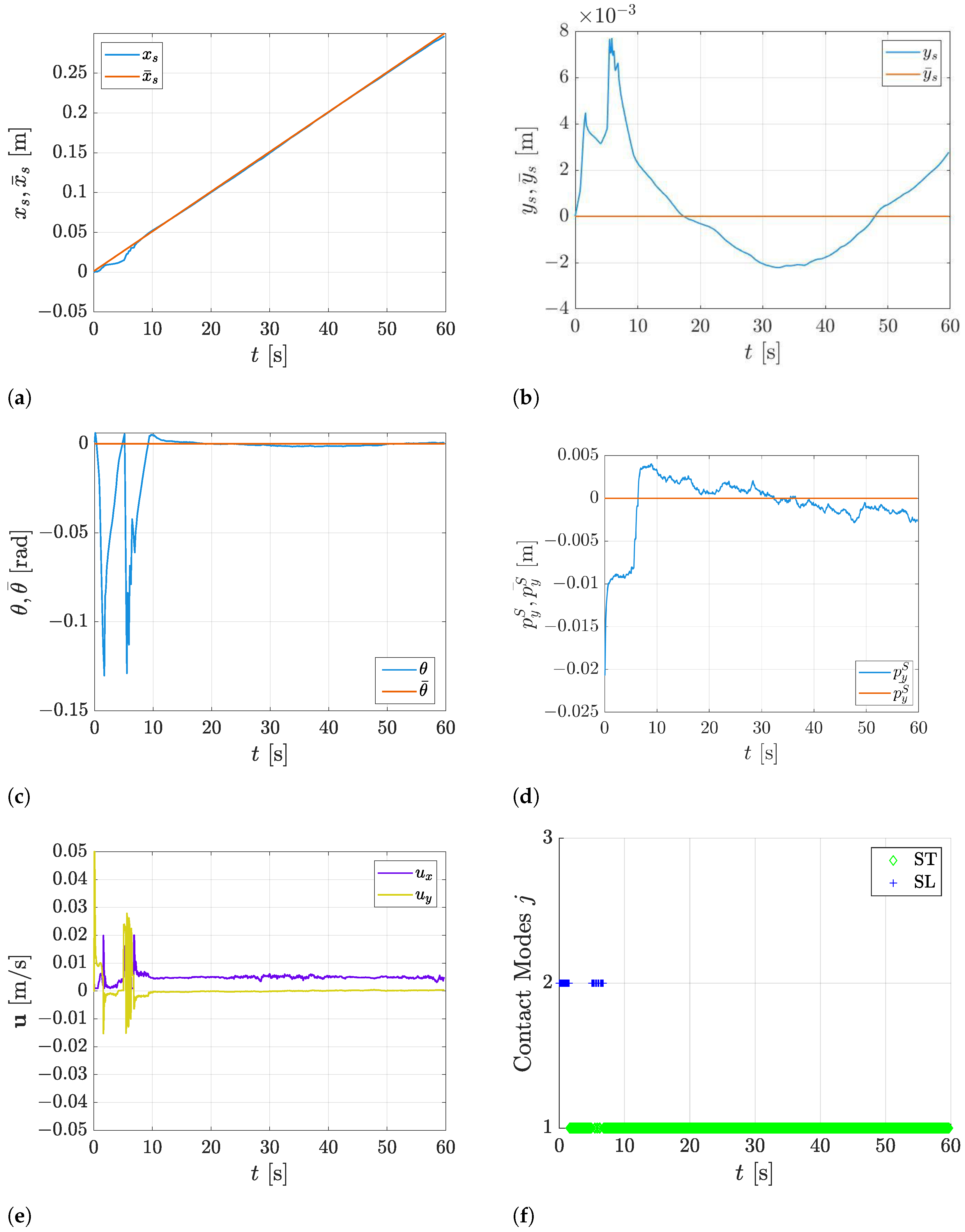
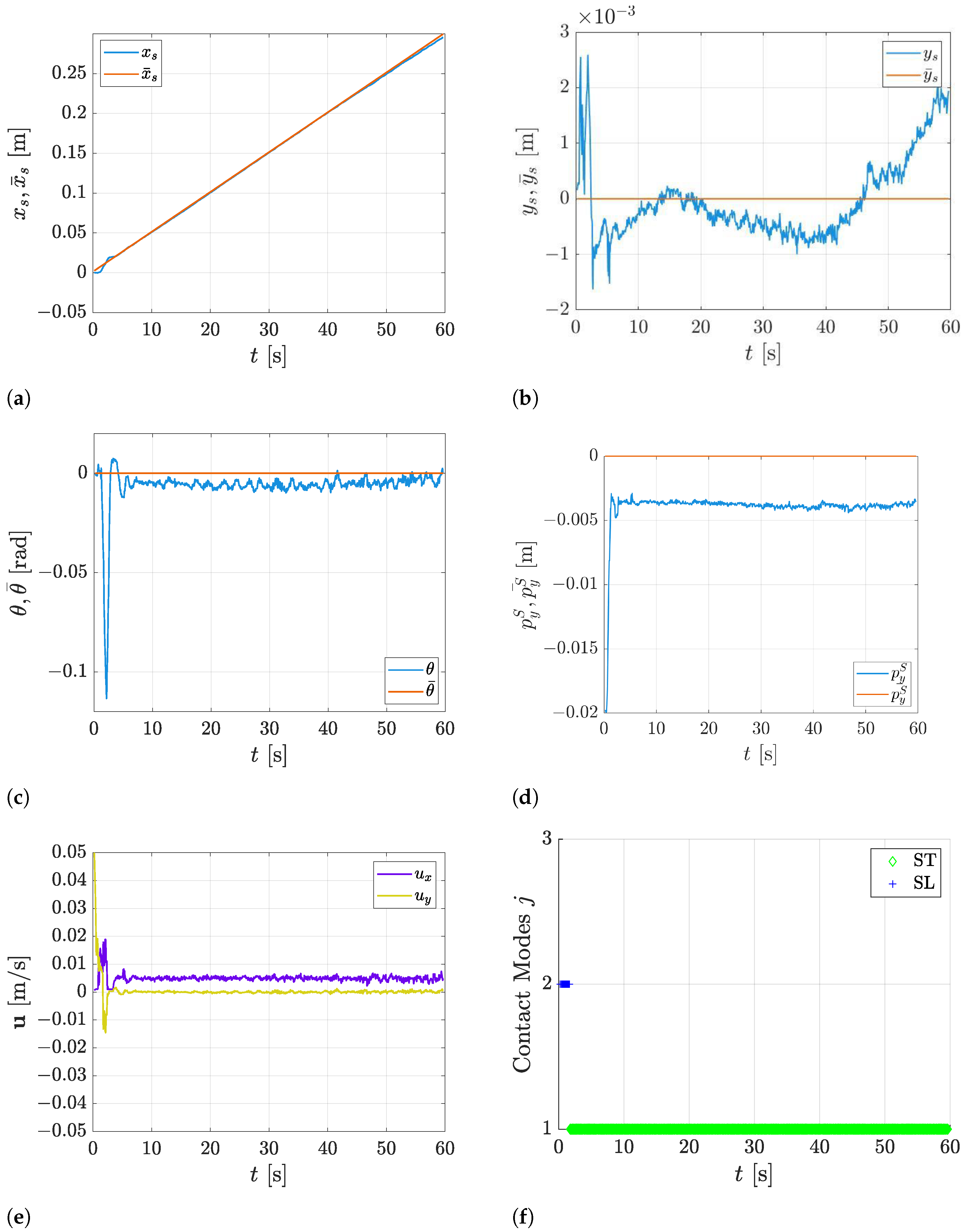
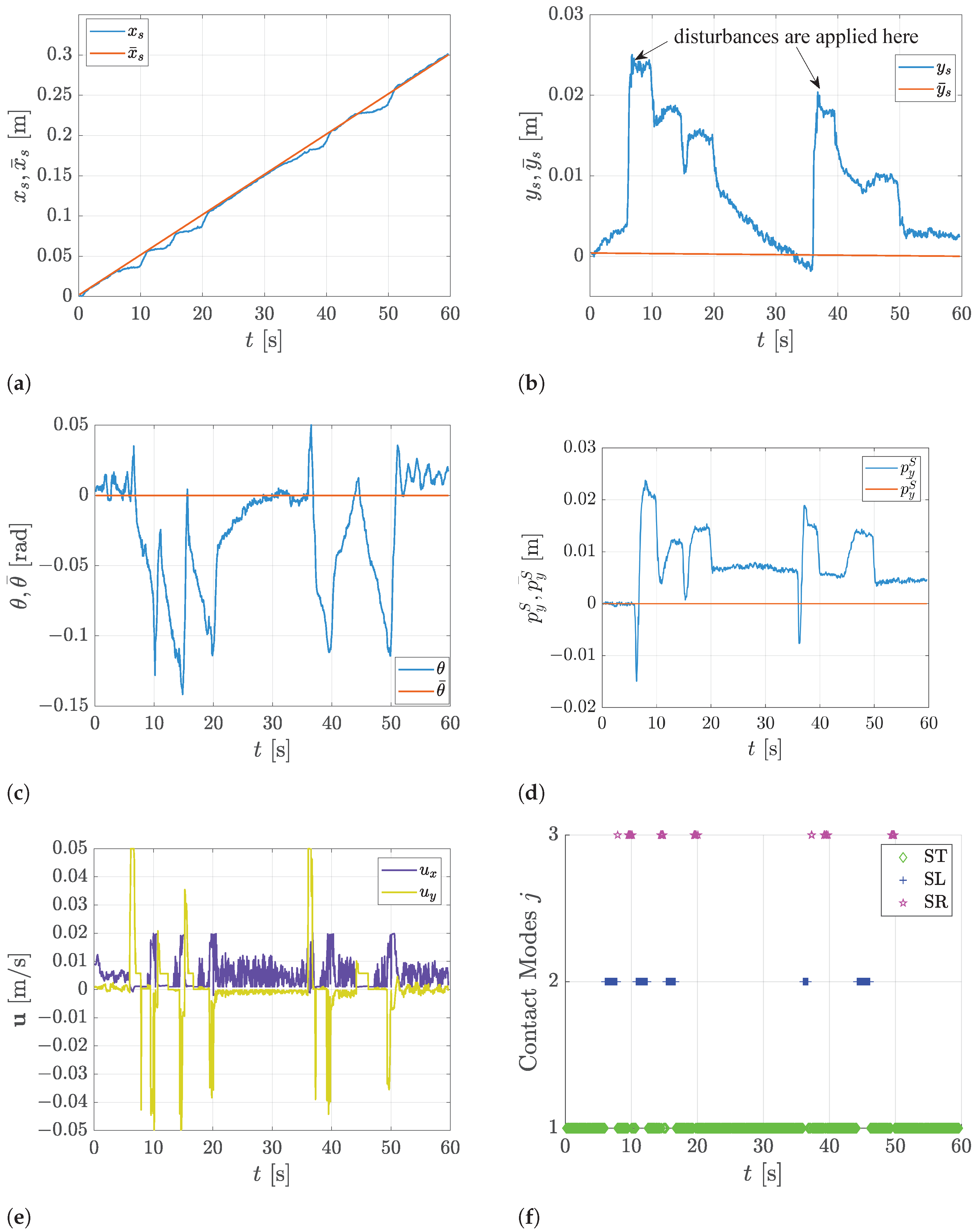
5.2. Straight Line Tracking with Disturbances

To test the robustness of the control system, the previous experiment has been repeated in a real-world setting by applying two disturbances to the system during the execution. The disturbances are applied by touching the object by hand, hence moving it from the desired path and varying $y_s$, as it can be appreciated in Figure 13b. The first touch, which causes a displacement of $0.024\mathrm{m}$, is applied after six seconds from the start of the task execution, while the second one, $0.02\mathrm{m}$ large, is applied about thirty seconds after the first one. Naturally, the effect of the disturbance affects all the state variables, causing a transient increase in the tracking error. In both cases, as soon as the disturbances act, a change of mode occurs: the contact modes in both the cases switch from the previous sticking contact mode to the sliding mode (Figure 13f). In this way, by applying a tangential velocity, which almost saturates to the imposed constraints, the robot is able to reject the disturbances, bringing the object back on track and achieving a steady-state error in the order of millimeters, as in the previous experiment. Note that, compared to the other state variables, in all the experiments a greater error on $p_y^S$ is recorded. This is reasonable considering the weight matrices used in the MPC designer. In fact, the value used to weigh $v_{py}^S$ is much smaller than the ones used to weigh $x_s$ and $y_s$, both in $\mathit{W}$ and ${\mathit{W}}_H$. This is because it is not important that $y_s$ follows the reference signal, but only that it does not exceed its constraints.

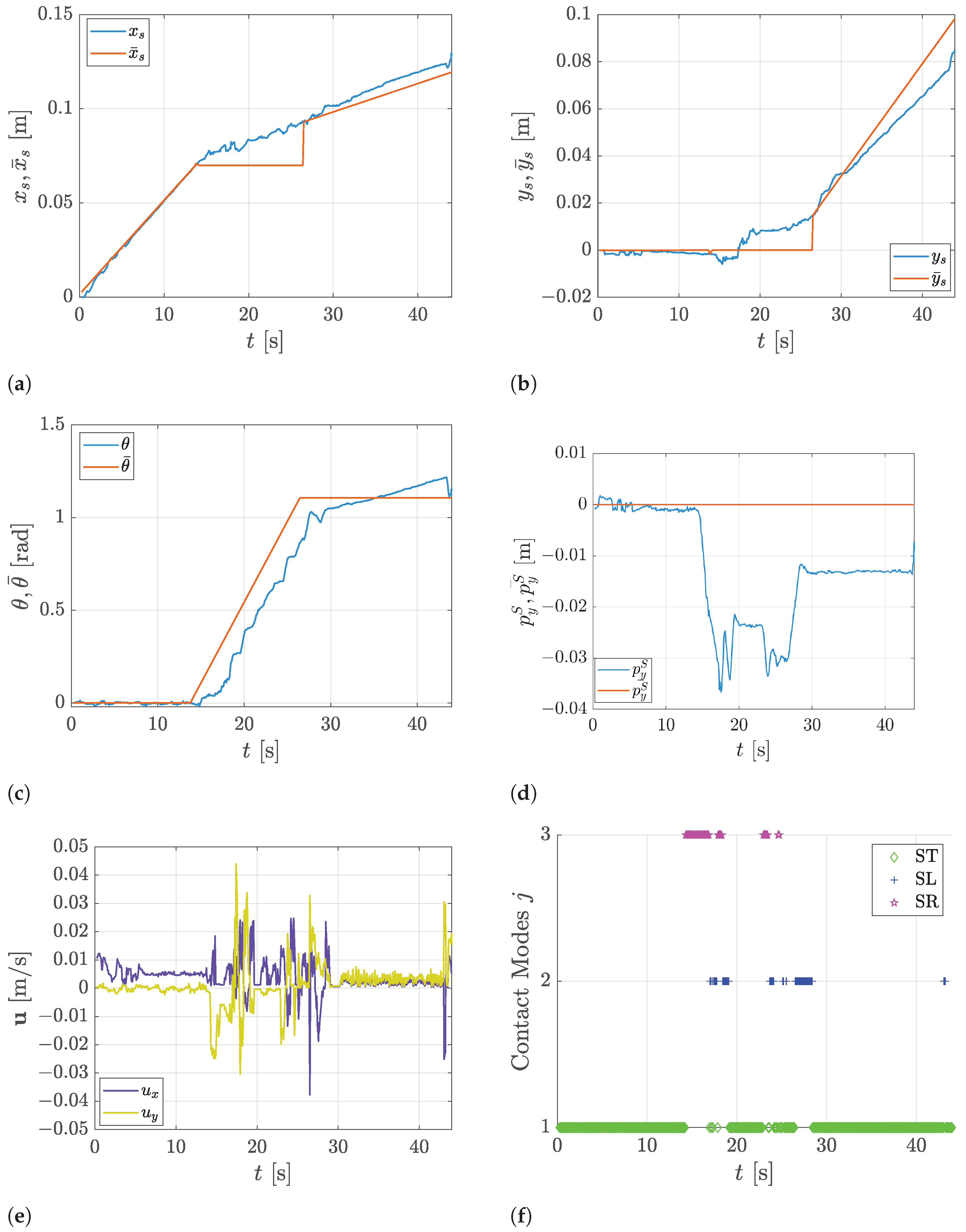
5.3. Trajectory Tracking

The following experiment is performed to demonstrate the utility of a pushing maneuver in a real-world application of robotic manipulation of fresh fruit. The task is performed by the robot by using the recognition system described in this paper and the overall pipeline in Figure 5.

Figure 14 shows the scenario of this experiment. The proposed robotic task consists in picking the red apple placed in a cluttered box and placing it in a container on its left. To recognize, grasp and place the fruit in the desired position, the pipeline described in Section 4 is adopted. In the considered situation (see Figure 14), the grasp of the apple is unfeasible due to the two fruit juice bricks very close to the apple. Indeed, the adopted grasp selection strategy, also due to the gripper design, cannot find a feasible solution to allow the pick of the target object without colliding with the obstacles in the scene. In this context, a non-prehensile manipulation is very helpful to successfully complete the proposed task by preliminary moving one of the obstacles.

By following the approach described in Section 3.4, a more complex trajectory has been generated using the points $P_1=\left[\begin{array}{cc}0.07& 0\end{array}\right]\mathrm{m}$ and $P_2=\left[\begin{array}{cc}0.12& 0.10\end{array}\right]\mathrm{m}$ and an angular velocity $\alpha$ equal to $5^{\circ }/\mathrm{s}$. With reference to (12), the overall trajectory is defined through

$$\mathit{X}=\left[\begin{array}{ccc}0.07& 0& 0\\ 0.07& 0& 1.1071\\ 0.12& 0.10& 1.1071\end{array}\right],$$

(16)

where the coordinates in the first two columns and the angles in the last column are expressed in meters and radians, respectively; therefore, three phases can be detected: the first one consists of a straight line, the second phase is a pure rotation and the third one is a new straight line.

Figure 15 illustrates the state evolution of the closed loop system, the control signals, and the contact mode chosen at each step. The tracking of the first segment takes place with high precision. However, when the system has to track the second part of the trajectory, which is a pure rotation, an error on $x_s$ and $y_s$ begins to accumulate. This is unavoidable since a pure rotation can be realized only by applying a moment to the object. To follow the angular reference a switch of contact mode is required, so that a tangential velocity is applied, but during this phase the normal velocity cannot be zero to avoid contact loss. Then, in the third part of the trajectory, the system returns to track a straight line in sticking mode with the desired nominal velocity. In the end, a low steady-state error is reached. Therefore, the results obtained from this experiment also test the ability of the designed control system to track a more complex trajectory using the strategy described in Section 3.4.

Finally, Figure 16 shows a series of screenshots of the overall pipeline of this experiment, reporting its most important steps. As shown in Figure 16e,f, thanks to the pushing maneuver performed in the previous step, the robot is able to pick the red apple without colliding with the other objects in the scene and place it in the container on its left as required by the task.

A video of all the experiments is available as Supplementary Material (Video S1).

6. Discussion and Conclusions

In order to highlight the utility of the pushing maneuver, several experiments have been conducted in addition to the previous ones evaluating the grasping success rate obtained by using the pipeline in Figure 5 in random cluttered scenes. Particularly, 15 cluttered scene configurations, containing one red apple and three juice bricks, were generated, and for each of them, the grasp of the apple, with the strategy described in Section 4.1, was attempted, allowing also the robot to push the obstacles in the scene as described in the pipeline in Figure 5 when necessary.

Both the apple and the juice bricks are enclosed in a circle of radius $r_{apple}$ = 0.04 m and $r_{juice}$ = 0.05 m, respectively, simply to ease the computation of the distance among all objects. In detail, the 2D positions of the juice bricks in the scene are generated by using a Gaussian distribution with respect to the frame placed in the center of the red apple, placed in a fixed position in the box. The random positions of the juice are generated while avoiding collisions with all other objects in the scene and in a rectangle of width 0.30 m (x direction), height 0.24 m (y direction) and centered in the center of the apple. The orientations of the juice bricks are kept fixed.

As a result, out of fifteen random scene configurations, seven of them (almost $50\%$) required the pushing maneuver to pick the apple, since the prehensile maneuver alone with the grasping selection strategy is not sufficient to complete the desired task without collisions. Figure 17 shows some of these configurations, in which the non-prehensile action has become necessary to allow the robot to grasp the red apple. In these cases, the juice brick selected to realize the pushing maneuver is the closest to the center of the apple.

These results allow us to claim that a combination of both prehensile and non-prehensile manipulation actions greatly enhances robot’s ability to act in complex scenarios, by doubling the fruit picking success rate with respect to a robotic solution not endowed with the pushing ability. On one hand, the approach proposed to perform robot control in both types of maneuvers is model-based. Complex physics-based friction models have been used to describe the dynamics of the objects being manipulated, both pushed and grasped. Such a priori knowledge allowed us to limit the number of parameters to be known by the controllers to few units. However, the friction model is limited to a uniform friction coefficient over the contact surface between the object and the support surface, which is assumed to be flat. Therefore, future work is needed to relax such assumptions. The control algorithm is based on a state-of-the-art MPC endowed with innovative enhancements such as a chattering avoidance strategy and a delay compensation algorithm, which significantly improved the robotic system performance. The main limitation of the control strategy is that inertial forces are neglected, hence only low acceleration maneuvers are possible. On the other hand, the proposed object perception system is based on a combination of deep neural networks and a geometric model useful to improve the accuracy in the 6D pose estimation. Even though the network architecture is characterized by a high complexity, it can be trained exclusively through synthetic data. Its generalization capabilities in the pose estimation have been achieved through the geometric model and the suitable exploitation of depth measurements. The results achieved so far are encouraging and urge the authors to pursue the method to achieve a better autonomy, e.g., by integrating AI reasoning methods to autonomously plan the pushing path and the grasping pose, and to exploit reinforcement learning methods to generalize the non-prehensile manipulation action to more complex contact conditions.

References

- Lynch, K.; Mason, M. Stable Pushing: Mechanics, Controllability, and Planning. Int. J. Robot. Res. 1999, 15, 533–556. [Google Scholar] [CrossRef]
- Yu, K.T.; Bauza, M.; Fazeli, N.; Rodriguez, A. More than a million ways to be pushed. A high-fidelity experimental dataset of planar pushing. In Proceedings of the 2016 IEEE/RSJ International Conference on Intelligent Robots and Systems (IROS), Daejeon, Korea, 9–14 October 2016; pp. 30–37. [Google Scholar] [CrossRef] [Green Version]
- Yu, K.T.; Leonard, J.; Rodriguez, A. Shape and pose recovery from planar pushing. In Proceedings of the 2015 IEEE/RSJ International Conference on Intelligent Robots and Systems (IROS), Hamburg, Germany, 28 September–2 October 2015; pp. 1208–1215. [Google Scholar] [CrossRef] [Green Version]
- Lynch, K. Estimating the friction parameters of pushed objects. In Proceedings of the 1993 IEEE/RSJ International Conference on Intelligent Robots and Systems (IROS’93), Yokohama, Japan, 26–30 July 1993; Volume 1, pp. 186–193. [Google Scholar] [CrossRef]
- Mason, M.T. Mechanics and Planning of Manipulator Pushing Operations. Int. J. Robot. Res. 1986, 5, 53–71. [Google Scholar] [CrossRef]
- Akella, S.; Mason, M. Posing polygonal objects in the plane by pushing. In Proceedings of the 1992 IEEE International Conference on Robotics and Automation, Nice, France, 12–14 May 1992; Volume 3, pp. 2255–2262. [Google Scholar] [CrossRef]
- Lynch, K.; Maekawa, H.; Tanie, K. Manipulation And Active Sensing By Pushing Using Tactile Feedback. In Proceedings of the IEEE/RSJ International Conference on Intelligent Robots and Systems, Raleigh, NC, USA, 7–10 July 1992; Volume 1, pp. 416–421. [Google Scholar] [CrossRef] [Green Version]
- Hogan, F.R.; Rodriguez, A. Reactive planar non-prehensile manipulation with hybrid model predictive control. Int. J. Robot. Res. 2020, 39, 755–773. [Google Scholar] [CrossRef]
- Hogan, F.R.; Rodriguez, A. Feedback Control of the Pusher-Slider System: A Story of Hybrid and Underactuated Contact Dynamics. In Algorithmic Foundations of Robotics XII: Proceedings of the Twelfth Workshop on the Algorithmic Foundations of Robotics; Springer International Publishing: Cham, Switzerland, 2020; pp. 800–815. [Google Scholar] [CrossRef]
- Costanzo, M.; Simone, M.D.; Federico, S.; Natale, C.; Pirozzi, S. Enhanced 6D Pose Estimation for Robotic Fruit Picking. In Proceedings of the 9th International Conference on Control, Decision and Information Technologies (CoDIT’23), Rome, Italy, 3–6 July 2023. [Google Scholar]
- Mason, M. Manipulator Grasping and Pushing Operations; Technical Report; Massachusetts Institute of Technology: Cambridge, MA, USA, 1986. [Google Scholar]
- Goyal, S.; Ruina, A.; Papadopoulos, J. Planar sliding with dry friction Part 1. Limit surface and moment function. Wear 1991, 143, 307–330. [Google Scholar] [CrossRef]
- Lee, S.H.; Cutkosky, M.R. Fixture planning with friction. J. Eng. Ind. 1991, 113, 320–327. [Google Scholar] [CrossRef]
- Bauza, M.; Hogan, F.R.; Rodriguez, A. A Data-Efficient Approach to Precise and Controlled Pushing. In Proceedings of the 2nd Conference on Robot Learning, Zürich, Switzerland, 29–31 October 2018; Billard, A., Dragan, A., Peters, J., Morimoto, J., Eds.; Volume 87, pp. 336–345. [Google Scholar]
- Kopicki, M.; Zurek, S.; Stolkin, R.; Mörwald, T.; Wyatt, J. Learning to predict how rigid objects behave under simple manipulation. In Proceedings of the 2011 IEEE International Conference on Robotics and Automation, Shanghai, China, 9–13 May 2011; pp. 5722–5729. [Google Scholar] [CrossRef]
- Byravan, A.; Fox, D. SE3-nets: Learning rigid body motion using deep neural networks. In Proceedings of the 2017 IEEE International Conference on Robotics and Automation (ICRA), Singapore, 29 May–3 June 2017; pp. 173–180. [Google Scholar] [CrossRef] [Green Version]
- Zeng, A.; Song, S.; Welker, S.; Lee, J.; Rodriguez, A.; Funkhouser, T. Learning Synergies between Pushing and Grasping with Self-Supervised Deep Reinforcement Learning. In Proceedings of the 2018 Proceedings of the IEEE International Conference on Intelligent Robots and Systems (IROS), Madrid, Spain, 1–5 October 2018; pp. 4238–4245. [Google Scholar]
- Hinterstoisser, S.; Cagniart, C.; Ilic, S.; Sturm, P.; Navab, N.; Fua, P.; Lepetit, V. Gradient Response Maps for Real-Time Detection of Textureless Objects. IEEE Trans. Pattern Anal. Mach. Intell. 2012, 34, 876–888. [Google Scholar] [CrossRef] [PubMed] [Green Version]
- Li, Y.; Wang, G.; Ji, X.; Xiang, Y.; Fox, D. DeepIM: Deep Iterative Matching for 6D Pose Estimation. In Proceedings of the European Conference on Computer Vision (ECCV), Munich, Germany, 8–14 September 2018. [Google Scholar]
- Rios-Cabrera, R.; Tuytelaars, T. Discriminatively Trained Templates for 3D Object Detection: A Real Time Scalable Approach. In Proceedings of the 2013 IEEE International Conference on Computer Vision, Sydney, Australia, 1–8 December 2013; pp. 2048–2055. [Google Scholar]
- Xiang, Y.; Schmidt, T.; Narayanan, V.; Fox, D. PoseCNN: A Convolutional Neural Network for 6D Object Pose Estimation in Cluttered Scenes. In Proceedings of the XIV Robotics Science and Systems Conference (RSS), Pittsburgh, PA, USA, 26–30 June 2018. [Google Scholar]
- Tremblay, J.; To, T.; Sundaralingam, B.; Xiang, Y.; Fox, D.; Birchfield, S. Deep Object Pose Estimation for Semantic Robotic Grasping of Household Objects. In Proceedings of the 2nd Conference on Robot Learning, Zürich, Switzerland, 29–31 October 2018; Billard, A., Dragan, A., Peters, J., Morimoto, J., Eds.; Volume 87, pp. 336–345. [Google Scholar]
- Hou, T.; Ahmadyan, A.; Zhang, L.; Wei, J.; Grundmann, M. MobilePose: Real-Time Pose Estimation for Unseen Objects with Weak Shape Supervision. arXiv 2020, arXiv:2003.03522. [Google Scholar]
- Lin, Y.; Tremblay, J.; Tyree, S.; Vela, P.A.; Birchfield, S. Single-Stage Keypoint-based Category-level Object Pose Estimation from an RGB Image. In Proceedings of the IEEE International Conference on Robotics and Automation (ICRA), Philadelphia, PA, USA, 23–27 May 2022. [Google Scholar]
- Pavlakos, G.; Zhou, X.; Chan, A.; Derpanis, K.G.; Daniilidis, K. 6-DoF object pose from semantic keypoints. In Proceedings of the 2017 IEEE International Conference on Robotics and Automation (ICRA), Singapore, 29 May–3 June 2017; pp. 2011–2018. [Google Scholar] [CrossRef] [Green Version]
- Wang, H.; Sridhar, S.; Huang, J.; Valentin, J.; Song, S.; Guibas, L.J. Normalized Object Coordinate Space for Category-Level 6D Object Pose and Size Estimation. In Proceedings of the IEEE Conference on Computer Vision and Pattern Recognition (CVPR), Long Beach, CA, USA, 15–20 June 2019. [Google Scholar]
- Manhardt, F.; Nickel, M.; Meier, S.; Minciullo, L.; Navab, N. CPS: Class-level 6D Pose and Shape Estimation From Monocular Images. arXiv 2020, arXiv:2003.0584. [Google Scholar]
- Wang, G.; Manhardt, F.; Shao, J.; Ji, X.; Navab, N.; Tombari, F. Self6D: Self-supervised Monocular 6D Object Pose Estimation. In Computer Vision—ECCV 2020; Vedaldi, A., Bischof, H., Brox, T., Frahm, J.M., Eds.; Springer International Publishing: Cham, Switzerland, 2020; pp. 108–125. [Google Scholar]
- Costanzo, M.; De Maria, G.; Natale, C.; Pirozzi, S. Design and Calibration of a Force/Tactile Sensor for Dexterous Manipulation. Sensors 2019, 19, 966. [Google Scholar] [CrossRef] [PubMed] [Green Version]
- Costanzo, M.; De Maria, G.; Natale, C. Two-Fingered In-Hand Object Handling Based on Force/Tactile Feedback. IEEE Trans. Robot. 2020, 36, 157–173. [Google Scholar] [CrossRef]
- Costanzo, M. Control of robotic object pivoting based on tactile sensing. Mechatronics 2021, 76, 102545. [Google Scholar] [CrossRef]
- Lepetit, V.; Moreno-Noguer, F.; Fua, P. EPnP: An accurate O(n) solution to the PnP problem. Int. J. Comput. Vis. 2009, 81, 155–166. [Google Scholar] [CrossRef] [Green Version]
- Morrical, N.; Tremblay, J.; Lin, Y.; Tyree, S.; Birchfield, S.; Pascucci, V.; Wald, I. NViSII: A Scriptable Tool for Photorealistic Image Generation. arXiv 2021, arXiv:2105.13962. [Google Scholar]
- Rao, C.; Wright, S.; Rawlings, J. Application of interior-point methods to model predictive control. J. Optim. Theory Appl. 1998, 99, 723–757. [Google Scholar] [CrossRef] [Green Version]
- Gurobi Optimization, LLC. Gurobi Optimizer Reference Manual. Available online: https://www.gurobi.com (accessed on 22 June 2023).
- Marchand, E.; Spindler, F.; Chaumette, F. ViSP for visual servoing: A generic software platform with a wide class of robot control skills. IEEE Robot. Autom. Mag. 2006, 12, 40–52. [Google Scholar] [CrossRef] [Green Version]