1. Introduction
Currently, there is a growing demand for studies on the viability of using Unmanned Aerial Vehicles (UAVs) in tasks that, until recently, were performed partially or exclusively by human workers [
1,
2]. Characteristics such as the versatility of flight modes, reduced dimensions, and the possibility of integration between sensors and actuators allow these vehicles to help in several areas, such as agriculture [
3,
4], industry [
5,
6], military [
7,
8], in the transportation of goods or people [
9,
10], in infrastructure inspection [
11,
12], forest monitoring [
13,
14], and rescue missions [
15,
16].
Information gathered by the sensors attached to the UAVs can contribute to decision making remotely, ensuring more secure operations [
17]. The main reason for introducing robotic systems in the mentioned tasks is to prevent operators from being exposed to hazardous environments, such as reservoirs containing toxic materials or mines with a potential risk of collapse. Another factor to consider is the repetitive and exhausting nature of specific tasks. The capability of these drones to cover large areas in a relatively short time allows them to help, for example, in the counting and monitoring of cattle [
18,
19].
Power line inspection is crucial for maintaining the quality of the power distribution. Potential failures or incidents in transmission networks can result in financial losses due to distribution interruption and accidents that can affect cities with the risk of environmental damage. Conventional approaches require workers in helicopters or direct contact with high-voltage components, are resource-demanding, often inefficient, and dangerous [
20,
21]. In Brazil, accidents in the electrical industry are, on average, 4.8 times greater than other sectors of the economy [
22]. Therefore, there is a demand for robotic systems that can support the identification of anomalies in distribution systems. UAVs are ideal for such activity due to the ease of coupling cameras and other sensors in addition to the capability of low-speed flights at a safe distance from the cables, allowing the acquisition of data and images that are significant for the maintenance of the system.
In this field of research, [
23] proposed a methodology for transmission line inspection in which a UAV takes off and proceeds to the mission starting point, determined by GPS readings. Then, the transmission cables are detected using a laser scanner, and the inspection is complete. Other studies have focused on establishing local positional control using image-based visual serving (IBVS) approaches. In these strategies, the features extracted directly from the images determine the relative position of the drone, and then a control technique is implemented. Therefore, Global Navigation Satellite System (GNSS) data are one option for locating power lines, but are often inaccurate [
24]. Ref. [
25] proposed a transmission line localization architecture that uses a histogram method of oriented segments to determine the position of lines. Next, proportional control is applied to align the drone with the lines. Ref. [
26] proposed an output feedback control for line tracking relative to a virtual image plane that compensates for the distortion created by the tilt of the drone body frame.
The traditional PID controller is still employed in many applications due to its simplicity of comprehension and ease of implementation, as it is not model-dependent. However, its applicability is limited to controlling nonlinear systems subject to measurement uncertainties, such as UAVs. Another problem faced by this approach is the necessity of controller gain tuning. Some authors employ intelligent techniques for PID controller gain tuning, such as Particle Swarm Optimization (PSO) [
27,
28] and Genetic Algorithm [
29,
30]. The sliding mode control is an adaptive tuning tool in [
31,
32].
The fuzzy logic theory has gained prominence in the controller tuning problem. Its advantage over the abovementioned techniques is the dynamic tuning of gains through fuzzy rules that are easy to interpret, to the detriment of complex equations that are usually difficult to comprehend. Thus, the controller gains adapt according to the behavior of the plant through the fuzzy membership functions. Hybrid approaches of type-1 fuzzy logic PID controllers (T1_PID) were employed for UAV control in [
33,
34,
35,
36].
Type-1 fuzzy models have difficulty dealing with uncertainties since they work with fixed membership functions. Therefore, the use of this technique in complex systems such as UAVs, which are subject to inaccurate measurements inherent to IBVS control systems, is worthy of attention. As a result, recent studies have introduced type-2 fuzzy systems, which model the uncertainties on antecedents and consequents through type-2 fuzzy sets via a Footprint of Uncertainty (FOU), the region enclosed by the union of all primary membership functions. Type-2 fuzzy logic as a PID tuning method was explored in [
37,
38]. In [
39], a comparison of hybrid fuzzy-PID systems was conducted, demonstrating the superiority of type-2 fuzzy in controlling UAVs in the presence of disturbances and uncertainties in the model.
This paper presents an interval type-2 fuzzy-PID (IT2_PID) controller for the transmission line follower problem through UAVs. The proposed methodology was compared with a conventional PID controller and a type-1 fuzzy-PID (T1_PID) controller. The fuzzy logic algorithm adaptively determines the proportional, derivative, and integrative gains as the UAV performs tracking. The trajectory is determined through images from a camera attached to the robot. For this purpose, the frame goes through a preprocessing step, and the lines are detected through the Probabilistic Hough Transform [
40]. The set of transmission lines should serve as a parameter for defining the trajectory to be followed. Thus, the strategy adopted is to compress all the pixels of the lines obtained into a single curve that will guide the drone. The RANSAC technique performs this process; this is a robust algorithm for curve parameter estimation from a subset of inliers from the complete data set. The advantage of this technique is its robustness against outliers, which are common in geometric shape detection in images. Thus, based on the curve obtained by RANSAC, the error variables are estimated and inserted into the control loop to keep the lines in the center of the image. The entire proposed approach was implemented using the ROS platform and validated through simulations performed by Gazebo. The main contributions presented in this paper can be summarized as follows:
The proposal of a power transmission line alignment and tracking methodology based on visual information integrated with a hybrid type-2 fuzzy-PID approach suitable for any multirotor vehicle.
The adaptive ability of the technique is demonstrated by the comparisons performed between a type-2 fuzzy-PID controller and its type-1 variant, a PID control tuned by Ziggler–Nichols, and a PID control with the average gains of fuzzy approaches.
The methodology is developed in Python with ROS integration making it easy to reproduce in different scenarios.
The proposed methodology is based on type-2 fuzzy logic, which has the advantage of dealing well with uncertainty, which is inherent to controls based on visual information.
The rest of this paper is organized as follows:
Section 2 describes the power lines tracking problem performed by the aerial robot and its mathematical foundations.
Section 3 presents the main outcomes and discusses the proposed methodology results. Finally,
Section 4 provides a brief conclusion and ideas for future work.
2. Problem Formulation
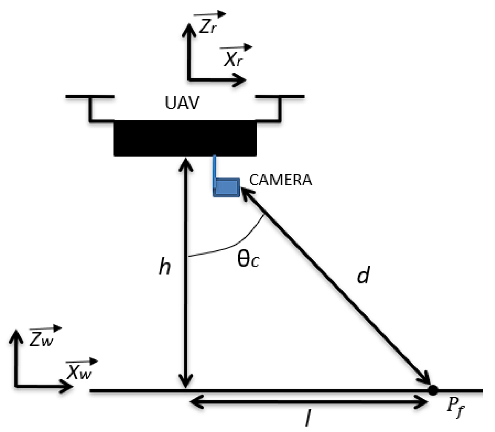
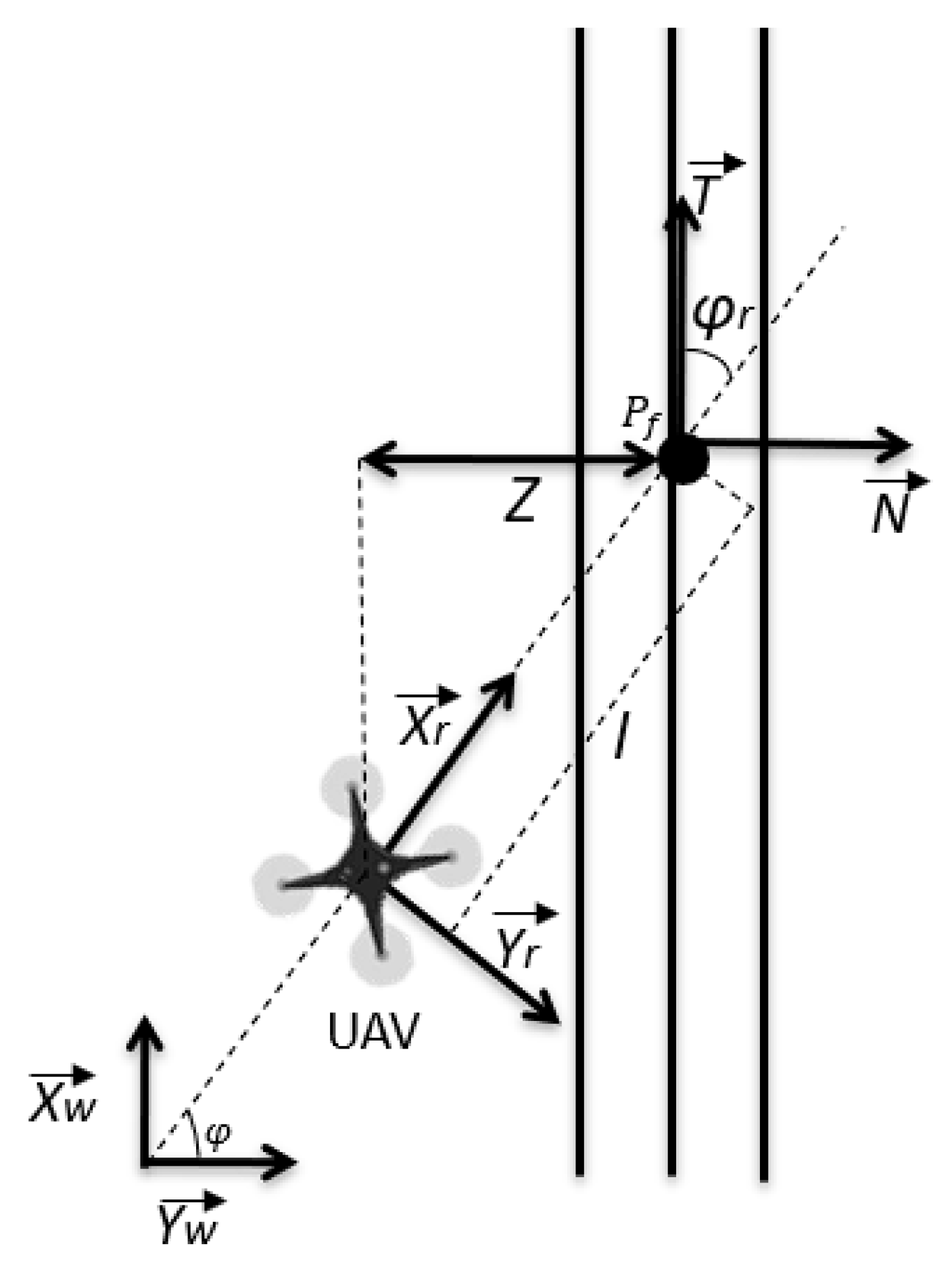
The methodology proposed in this paper is in the Image-Based Visual Servo (IBVS) control category, which relies on visual information extracted in the image plane, providing the control actions to be applied. In other words, the detected straight lines in a frame serve as a parameter for the determination of the drone’s position in relation to the power lines and, thus, the strategy adopted for trajectory tracking involves keeping the detected lines in the center of the image with their orientation perpendicular to the lower portion of the frame.
Figure 1 and
Figure 2 display the lateral and superior views of the proposed problem, respectively.
is the point of the path used to compute
Z,
h is the height of the UAV relative to the power lines,
is the tilt between the camera and the vertical axis of the UAV,
l and
d are the distances between the projection of the UAV on the transmission lines plane and the position of the camera to point
, respectively. The vectors
,
, and
are related to the world frame
W, while
,
, and
are related to the UAV frame
R.
is the vector parallel to the lines, while
is a vector perpendicular to
.
is the UAV’s orientation in relation to
W.
Table 1 presents the nomenclature used in this paper.
Based on this background, the proposed control methodology focuses on the minimization of two inputs in an uncoupled approach, consisting of one controller for the lateral error (
Z) that indicates how far the UAV is away from the center of the frame, and the second one for the angular error (
) that represents the angular deviation between the UAV and the power lines.
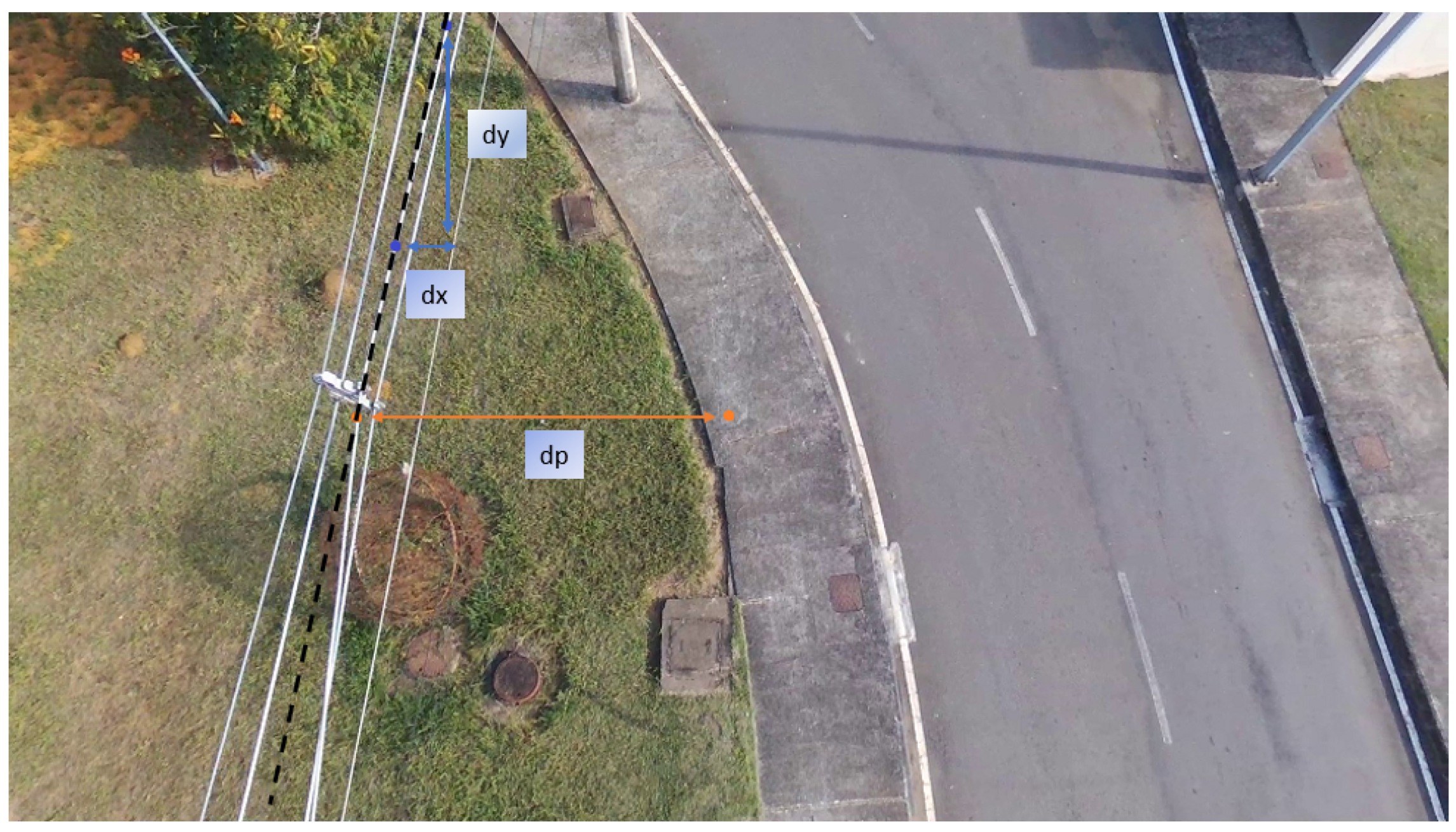
Figure 3 illustrates how to calculate these errors through visual information extracted from an image containing transmission power lines.
The position and orientation errors are estimated with Equations (
1) and (
2).
where
and
are the latitudinal and longitudinal lengths for the trajectory slope estimation,
is the distance between the trajectory and the center of the frame in pixels, and
k is a conversion factor from pixels to meters (
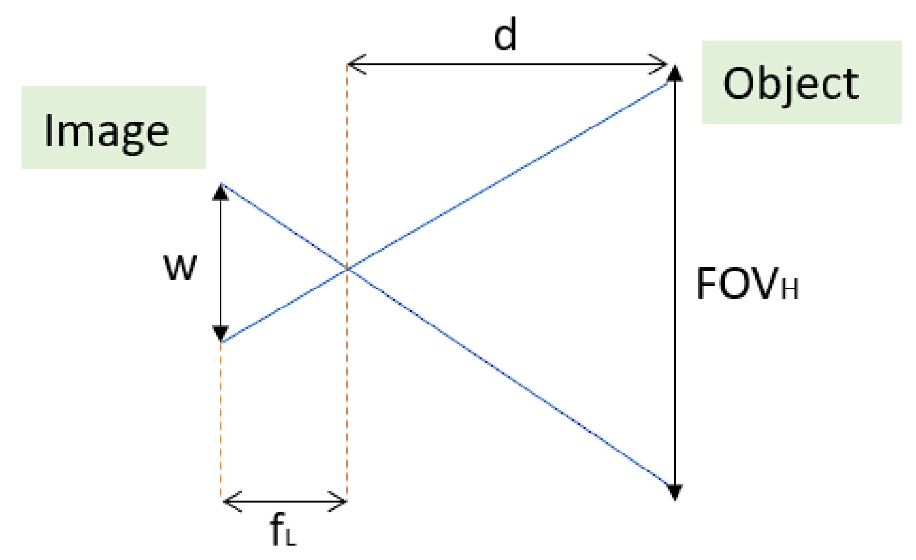
). Equations (
3) and (
4) present the relationships that compute
k. An illustration is shown in
Figure 4.
where
is the focal length of the camera,
is the camera horizontal field of view, and
w is the object width in the image. It is assumed that the height
h is known during the tests and that all transmission lines are within the camera’s field of view, which must be pointed downwards.
Note that controlling the x, y, and z inertial positions and orientation of a UAV is achieved by adjusting its rotor speeds. In this manner, the dynamics of a quadcopter can be interpreted with four velocities: pitch (u), roll (v), yaw (r), and thrust (t). The trajectory tracking problem introduced in this research work considers that the aircraft has a constant pitching velocity u. v must be estimated to minimize Z, whereas r minimizes . Therefore, an IT2_PID controller was developed for each velocity (IT2_PID_v and IT2_PID_r), with each controller working independently, receiving the desired reference and the respective error value and then generating roll and yaw velocities. A classic PID controller was also employed to keep the UAV under a constant altitude relative to the lines. The rotors are controlled by an internal control loop which is handled by the FCU (Flight Control Unit) via a mixing algorithm that receives the four velocities (u, v, r, and t) and translates them into commands for the actuators that control the rotors.
2.1. Image Processing
The parameters Z and must be defined accurately throughout the flight to prevent the UAV from unwanted oscillations or undesirable routes. A difficulty in computing these variables is caused by the presence of noise in the images, which may induce the rectilinear segment detection techniques to assume spurious features as straight lines or not detect them. To mitigate the effect of noise and increase the detectability of the lines, the obtained frame at a given time t passes through an image preprocessing step.
First, the frame passes through a color space conversion from RGB to grayscale. Next, a Gaussian blur is used to smooth the color transitions in the image frame, reducing the noise interpreted as straight lines. Finally, the image undergoes a contour detection step through the Canny edge detector. This process reduces the quantity of information in the image and, consequently, the computational effort.
2.2. Line Detection and Trajectory Parameter Estimation
Following image processing, the next step is power line detection. The lines are detected through the Probabilistic Hough Transform, a low-computational-cost technique for determining geometric patterns in images based on a scheme of voting accumulators containing candidate regions for the object to be detected. The difference between this approach and the classical Hough Transform is the selection of a random subset of edge points, which ensures less computational effort [
40]. In images of environments containing transmission lines, these features are expected to be highlighted against the other elements. However, asphalt markings or concrete structures can also be treated as straight elements and must be addressed as outliers to determine the path.
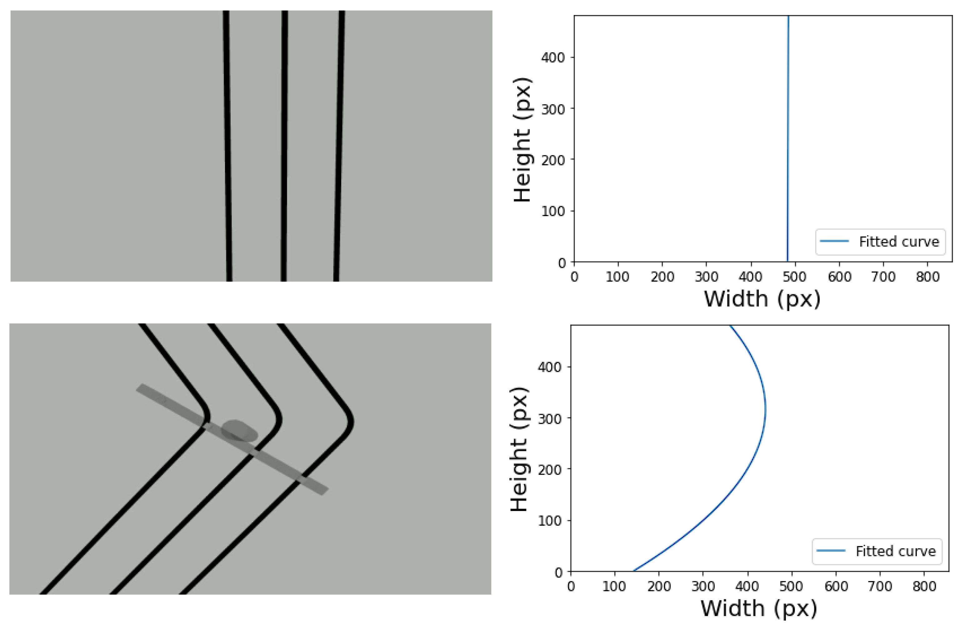
Following the transmission line detection, a binary image is created in which white pixels correspond to the detected lines. In aerial transmission line imaging scenarios captured by UAVs, the resulting binary mask is generally represented by three or more aligned straight lines corresponding to the transmission cables and other scattered rectilinear elements in the image. Considering these characteristics, the path to be followed by the UAV can be computed through a model-fitting technique. The method employed in this work was the RANSAC (Random Sample Consensus) algorithm. One characteristic that underlies such an approach is its robustness in the presence of outliers, since the model parameters can be estimated using a minimum sample of data.
Although the path is often rectilinear, a second-order curve was used to model the trajectory. The reason for this approach is that regions between two transmission poles can result in an abrupt change in the path orientation. Considering the path as a curve smooths these transitions, allowing navigation without significant oscillations.
Figure 5 exemplifies the trajectory estimation processes in two scenarios simulated with the Gazebo simulator.
2.3. Fuzzy Logic—PID Controllers
The hybrid approach of PID with fuzzy logic controllers combines the simplicity and robustness of traditional PID controllers with the capability of the fuzzy systems to introduce linguistic rules to the model, enabling it to behave in distinct ways based on the different input signals fed to the system. Therefore, the role of the fuzzy algorithm is to operate as an adaptive mechanism, adjusting the PID gains according to the current state of the plant.
In [
34], a type-1 fuzzy PID controller (T1_PID) was proposed for the positional control of a UAV as a starting point for the proposed methodology. The main difference is the replacement of the type-1 with a type-2 fuzzy logic block (IT2_PID). The internal architecture of this approach is similar to the T1_PID controller, except for replacing type-1 fuzzy sets (T1_FS) with type-2 fuzzy sets (T2_FS) and adding a type-reduction stage. A type-2 fuzzy set (
) can be characterized by its type-2 membership function as follows:
can also be written as
where
denotes the union of all admissible values for
x and
u.
is known as the primary membership of
x, while
is a type-1 fuzzy set referred to as the secondary set i.e.:
. Equation (
8) defines the Footprint of Uncertainty (FOU), which, as the name suggests, is the region that encloses the system input and output uncertainties.
The
of a type-2 fuzzy set is enclosed by the lower membership function (LMF) and the upper membership function (UMF) denoted by
and
, which are defined as follows:
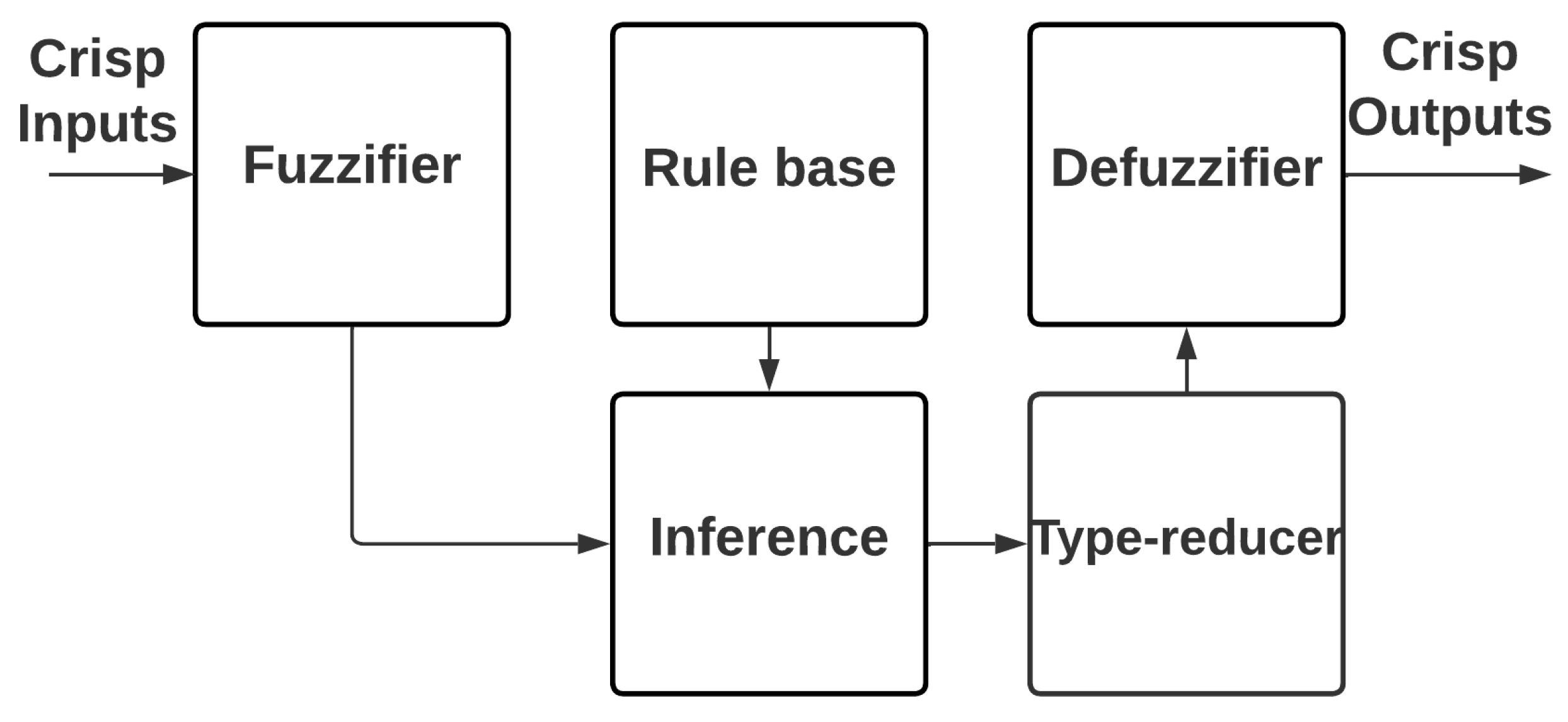
The following steps organize the type-2 fuzzy logic block:
Figure 6 provides a type-2 fuzzy inference system diagram.
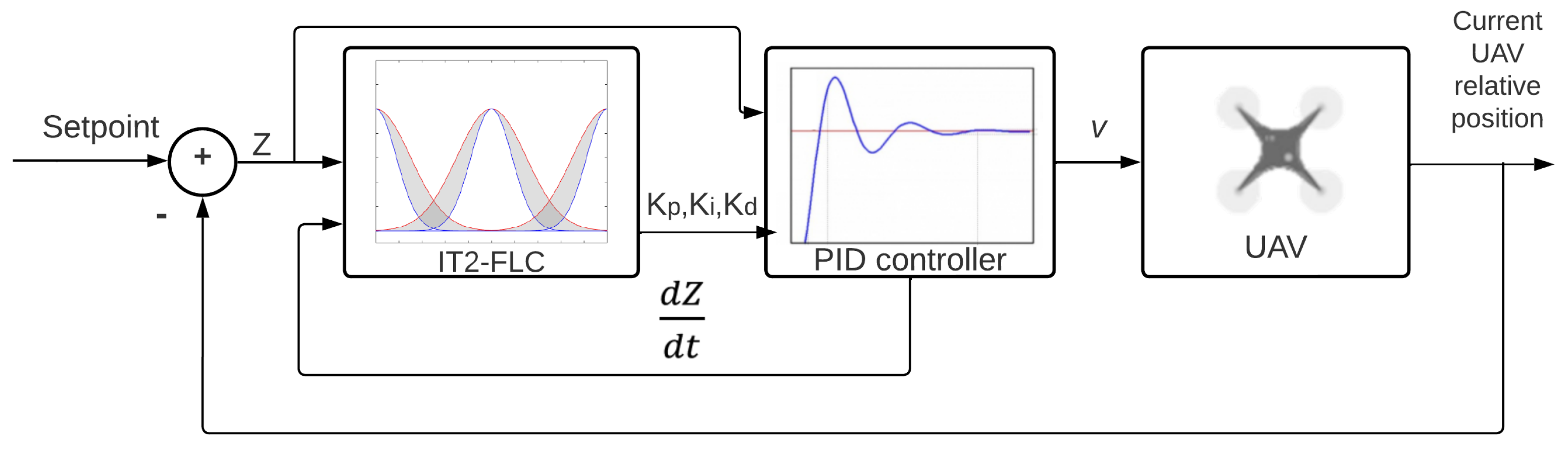
In this work, two type-2 fuzzy-PID controllers, IT2_PID_v and IT2_PID_r, were adopted. The first is related to the lateral error
Z, which also considers its time derivative, and the second is related to the angular error
and its derivative. Both operate independently to minimize errors simultaneously as the UAV follows the trajectory.
Figure 7 displays the schematic of the IT2_PID control used to control the input variable
Z.
,
and
are the proportional, integrative and derivative gains.
v is the roll velocity. The controller for the
error is similarly built.
Table 2 presents the fuzzy rules used in this paper, based on the rules presented by [
34]. The errors are addressed as small, medium, and large, while the derivative of the error can be either positive, negative, or zero. The consequents shown in the table refer to the set (
,
, and
), which can assume small (L), medium (M), and large (B) values, indicating the gains of the PID controller. The integrative gain
is obtained from the formula given by Equation (
19) in which
is a weighting factor.
The upper and lower bounds of the controller gains were established according to [
34,
42]. The derivative and integrative gains are discarded, and the proportional gain is increased to the point that the plant produces consistent oscillations. Thus, the values of the ultimate gain
and oscillation period
can be calculated. For the
controller, the values obtained were
and
s, whereas for
,
and
s.
The upper (
,
) and lower (
,
) limits of the gains are then calculated using Equations (
20)–(
23).
Finally, compression of the PID controller gain range is performed for a greater smoothing of the UAV’s movements. Thus, the bounds
,
,
, and
are obtained with Equations (
24)–(
27).
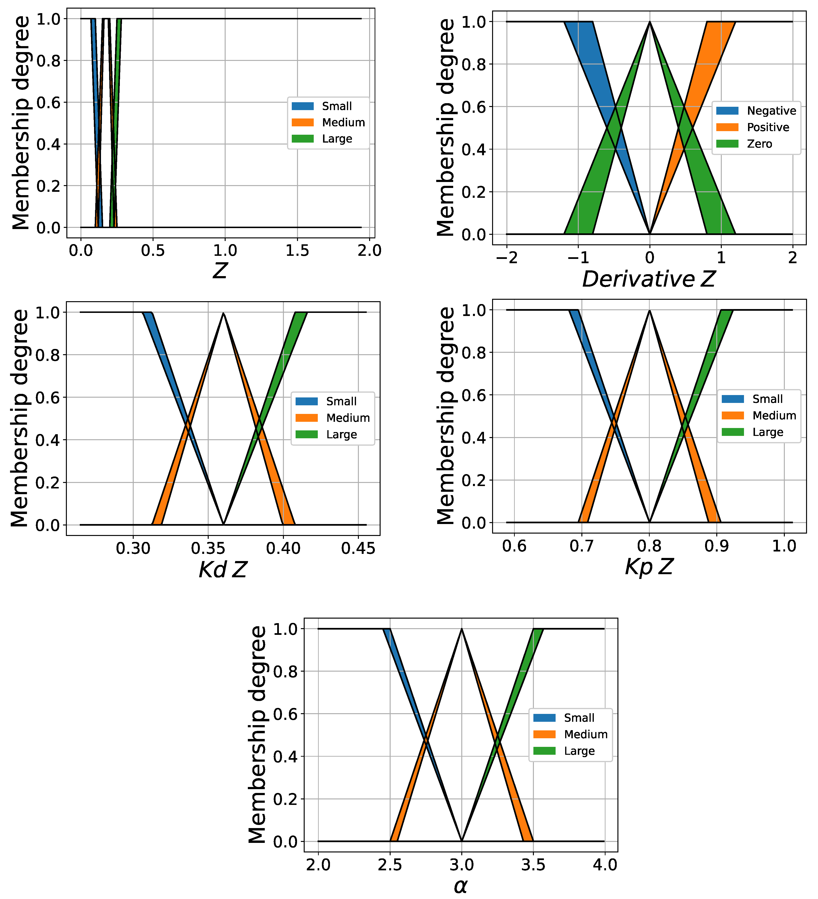
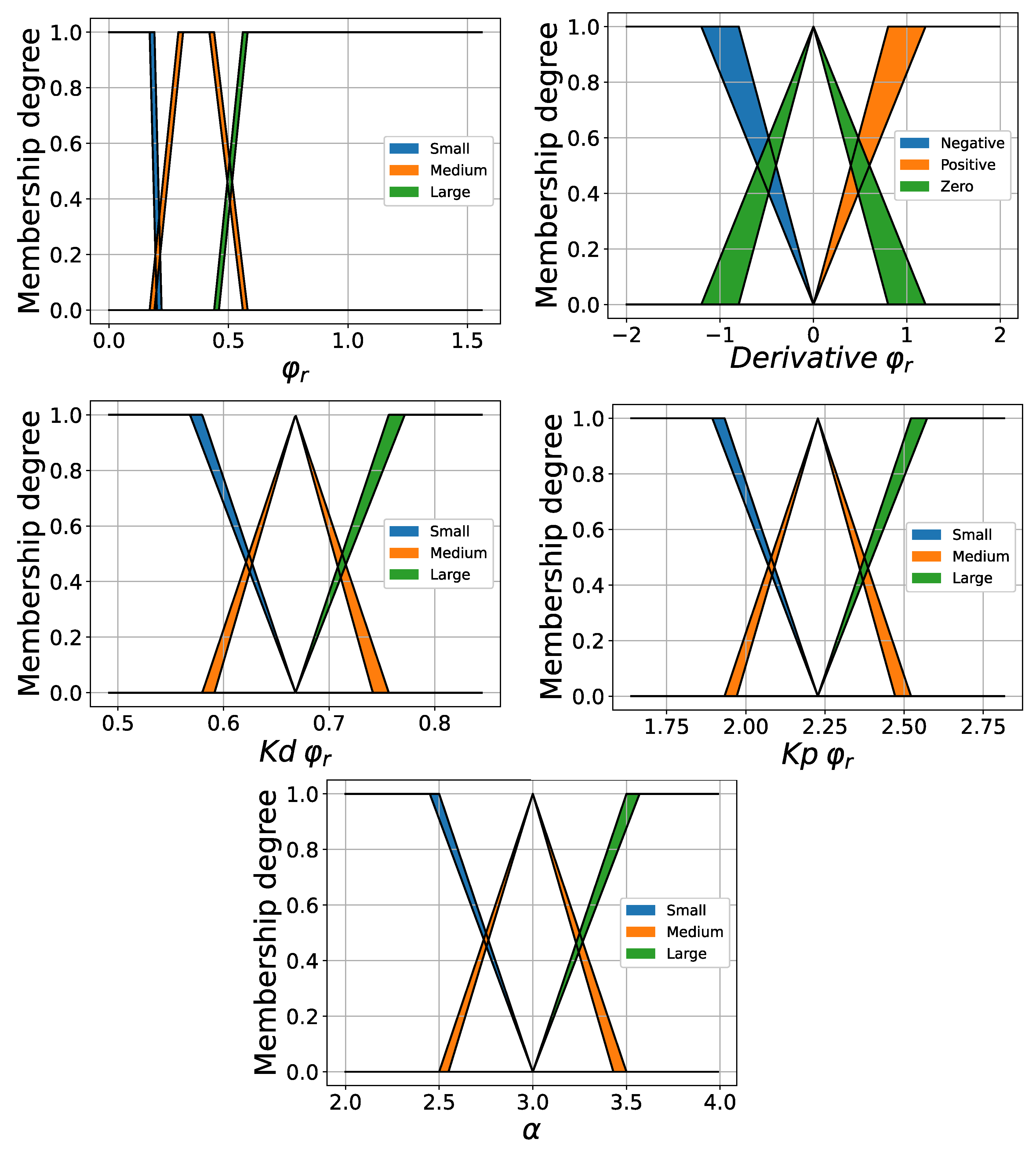
The input variables (i.e., errors and time derivatives) are transformed into fuzzy sets through the fuzzification process represented by the membership functions shown in
Figure 8 and
Figure 9. Finally, the outputs are subjected to a defuzzification stage to establish precise gain values.
3. Results and Discussion
The results presented in this section were obtained through Gazebo. This open-source robotic simulator enables the interaction between simulated sensors and robot actuators and integrates these robots with three-dimensional models. The communication between the sensors and actuators with the simulator is accomplished through the framework ROS.
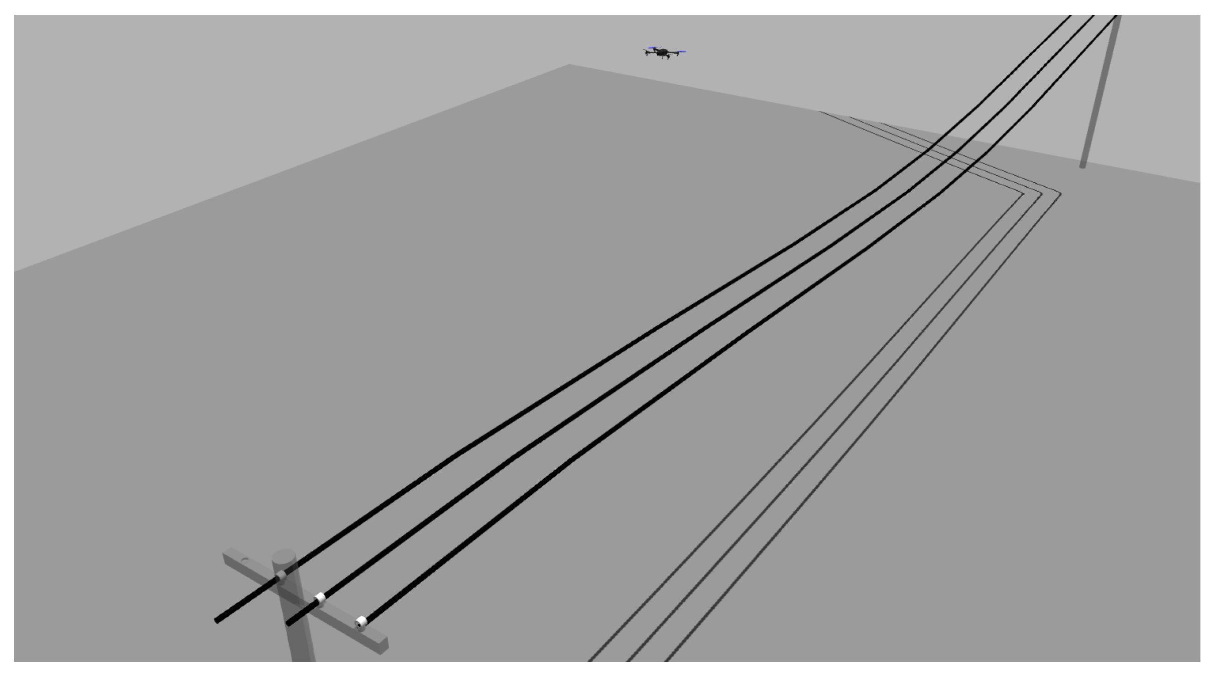
For this purpose, a scenario was developed consisting of transmission towers connected by power cables, as seen in
Figure 10. The UAV was simulated via a PX4 flight controller through Software-in-the-Loop (SITL) simulation. The control node proposed in this paper receives visual information from the frontal camera attached to the UAV, estimates the relative position to the lines, and calculates the PID gains that are converted into a velocity command, which is sent to the light management unit (FMU) through an ROS driver, the MAVROS. It is worth noting that the fuzzy controllers were developed using the Python library PyIT2FLS [
43].
The tests were performed on a computer with an Intel Core i5-10400F processor, an AMD Radeon RX 5600XT graphics card, and 16 GB of RAM. The operating system is Ubuntu 20.04.5 LTS 64-bit with ROS Noetic.
3.1. Horizontal Controller
Initially, the experiments were conducted involving the lateral control of the drone. For this purpose, the drone was positioned four meters above the lines, with a one-meter offset from the middle cable. The proposed controller, IT2_PID, was compared with a similar type-1 controller (T1_PID), the classic Ziegler–Nichols PID controller, and a PID controller using the mean gains assumed for the fuzzy approaches. The reason for this analysis is to investigate the capability of the proposed controller to adapt to different input scenarios compared with fixed-gain approaches.
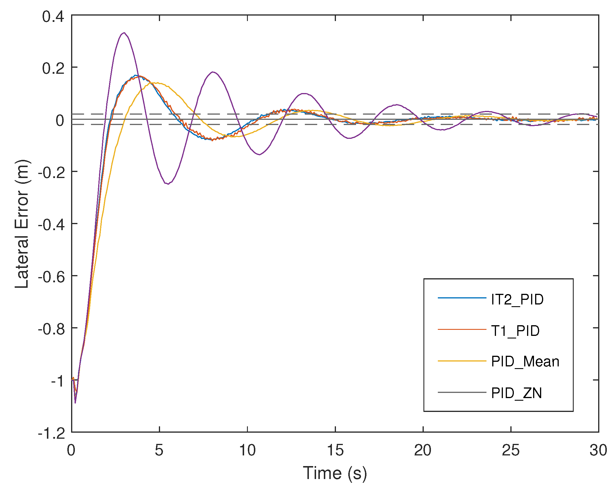
Table 2 shows the rule sets for both fuzzy approaches. Each controller was tested 50 times. The profile of the mean error over time is provided in
Figure 11. The solid line indicates the setpoint, while the dotted lines indicate the thresholds of the steady-state region.
Table 3 presents the quantitative results of the tests. IAE is the integral absolute error,
is the maximum peak,
is the peak time,
is the settling time, and
is the steady-state error. Additionally, the runtime for each controller was computed.
From the graphical analysis, it is seen that the four controllers could keep the UAV close to the established setpoint. However, the PID_ZN control displayed a high overshoot with higher oscillations, which is undesirable in UAV applications. The controllers IT2_PID and T1_PID presented lower values of IAE, which evaluates the absolute error throughout the test, with a slight advantage for the type-2 fuzzy version. The smallest value for the maximum peak was achieved by the PID_Mean control, despite higher values for the peak and accommodation times compared to the adaptive approaches. These findings justify the employment of fuzzy models to adjust the parameters compared to fixed-gain approaches. It is important to note that there are minor inconsistencies in the estimation of the lateral error in scenarios where the UAV has a certain degree of tilt, especially when the lines are near the end of the camera’s field of view. This effect was mitigated through an image rectification process, which employs a rotation matrix to correct the image perspective. Despite this behavior, the proposed controller kept the UAV close to the desired setpoint.
When comparing the two fuzzy approaches, the IT2_PID has superior results in all observed metrics based on mean values despite, as expected, having a longer processing time. However, it did not impact the overall system, which processes the information and sends velocity commands with a frequency of 10 Hz.
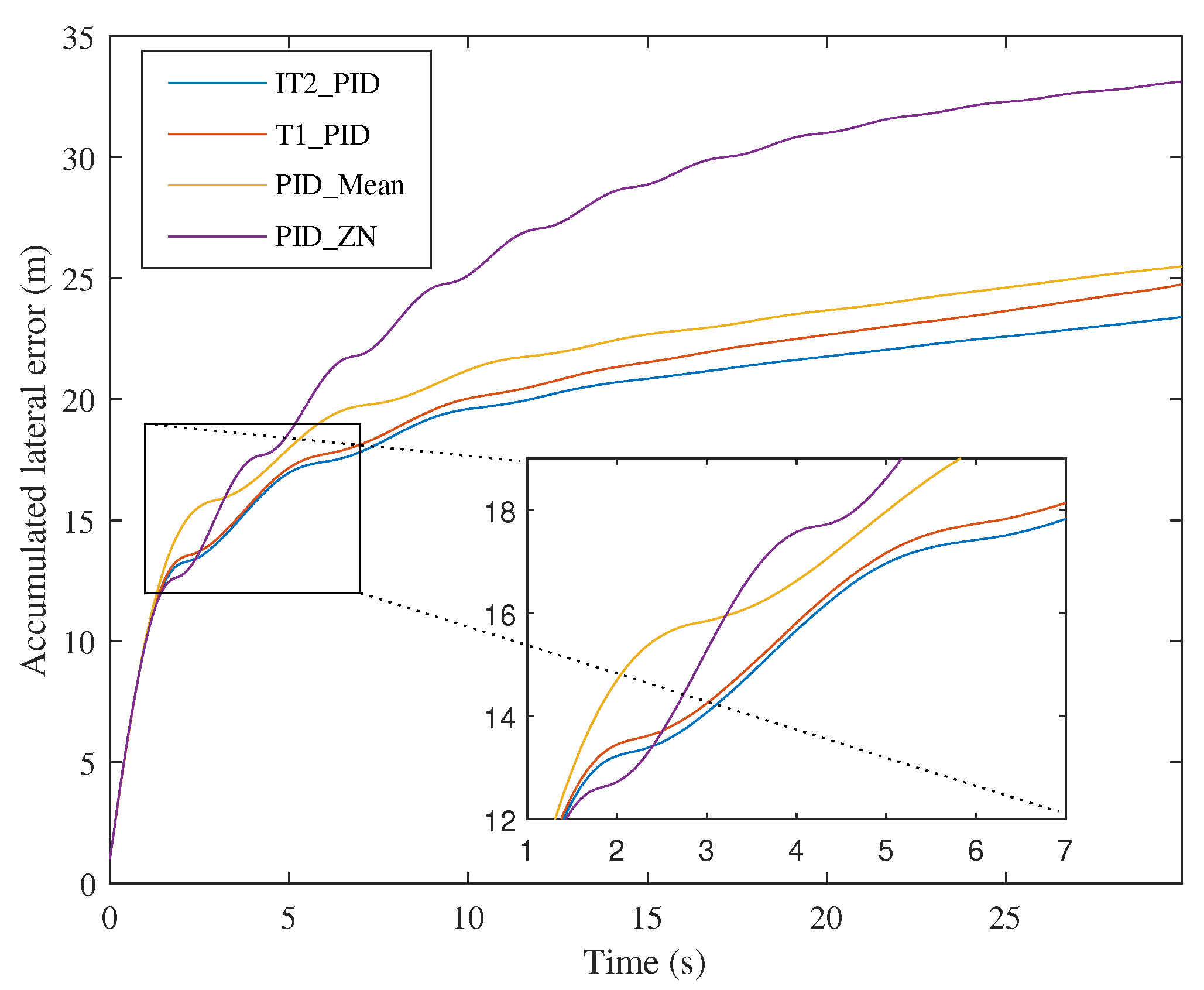
Finally, the accumulated error, which shows how far the UAV is from the desired position over the test period, is given in
Figure 12. All controllers display a similar behavior until approximately 1.4 s, when fixed-gain controllers exhibit more significant error variations. At 2.0 s, the distinction between the fuzzy approaches can be noticed, with the difference increasing throughout the steady state.
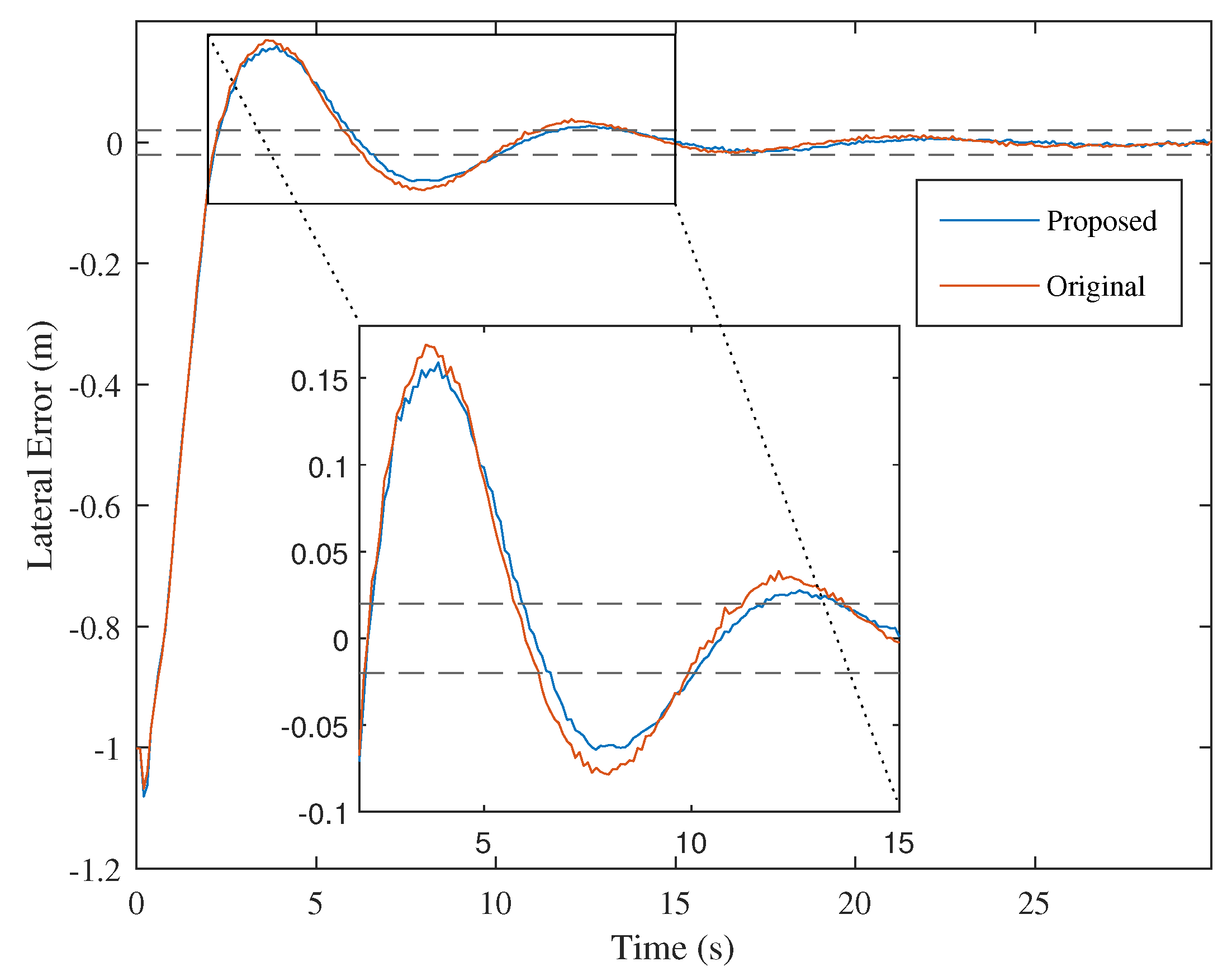
3.2. Modifications on Fuzzy Rules
By examining the set of rules expressed in
Table 2, proposed by [
35], it is possible to imply that the controller behaves uniformly in instances where the derivative of the error is either negative or positive, that is, whenever the absolute error decreases or increases, respectively. With this background information, some changes to the rule set were proposed to make the controller more aggressive as the UAV moves away from the setpoint and moves more smoothly as it heads toward it. Additionally, the derived gain was reduced for minor errors. Therefore,
Table 4 presents the new proposed rule set.
The graphical results of this modification are presented in
Figure 13, and the quantitative data can be seen in
Table 5.
From the graphical analysis, the rule set modifications could induce a slight reduction in the UAV oscillation in the transient regime. Such reduction can also be noticed in the quantitative results, with the reduction in the IAE and for the mean values. and processing time remain substantially unaffected.
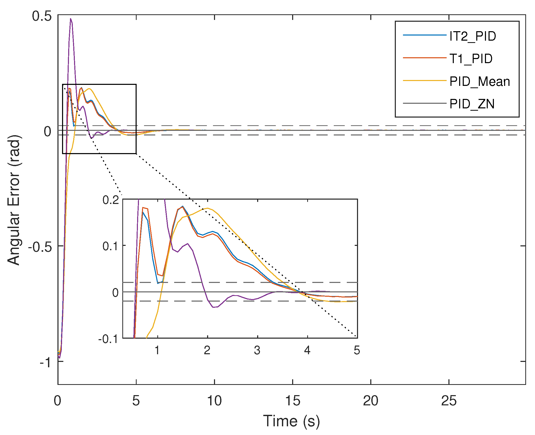
3.3. Angular Controller
Subsequently, an angular controller was introduced to maintain the UAV in parallel alignment with the power transmission lines. For the tests, the UAV was positioned at a height of 4 m from the lines with an angular deviation of
relative to the power lines. The membership functions for the fuzzy approaches are shown in
Figure 9, while the used rule set is presented in
Table 4.
Figure 14 shows the evolution of the error over time, while
Table 6 presents the quantitative measurements. As observed for the lateral error, the PID_ZN controller exhibited a significant main peak value, an expected behavior due to the aggressive nature of this type of controller. In comparison to the other approaches, it can be observed that the fixed-gain PID has the lowest peak maximum value; however, the integral of the absolute error is considerably higher than the adaptive gain controllers.
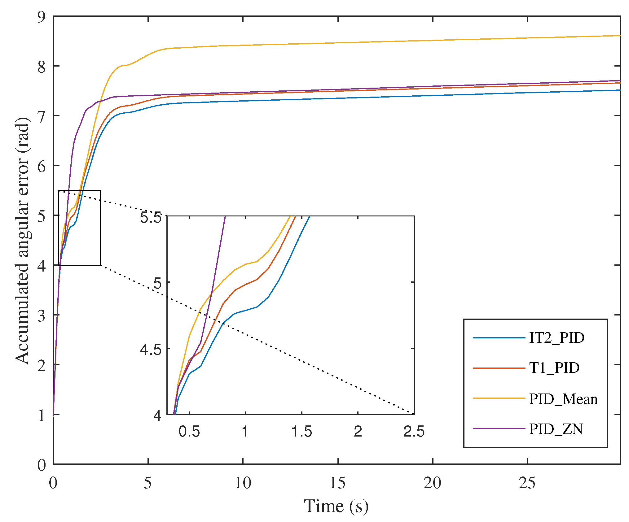
As observed for the lateral controller, the IT2_PID controller has outperformed the T1_PID over both the IAE and the
considering the mean values. This can also be noted by a slight reduction in the error deviation. From
Figure 15, it can be noticed that the difference in the cumulative error between the two methods was again in the transient state of the system, remaining relatively unchanged throughout the steady state. At approximately 1.5 s, the cumulative error of the PID_Mean increases, which emphasizes the capability of adaptive models to deal with several different settings.
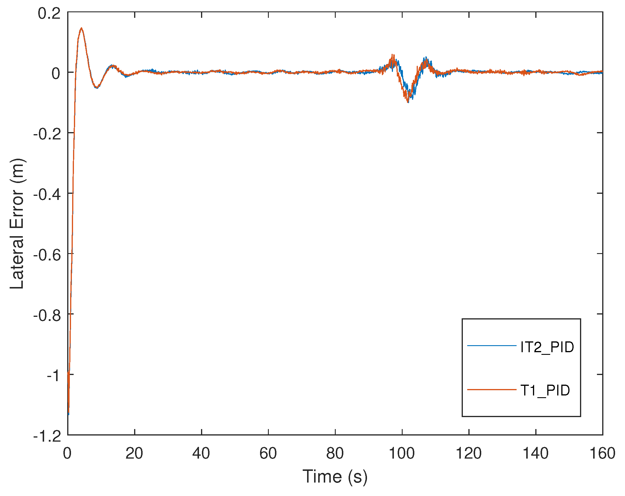
3.4. Simulation of an Inspection Mission
Finally, a simulation of a transmission line inspection mission was carried out. For this purpose, the UAV starts the tracking at a lateral offset of 1 m with an angular error of 0.75
. The drone follows the trajectory of three transmission towers connected by three cables, as shown in
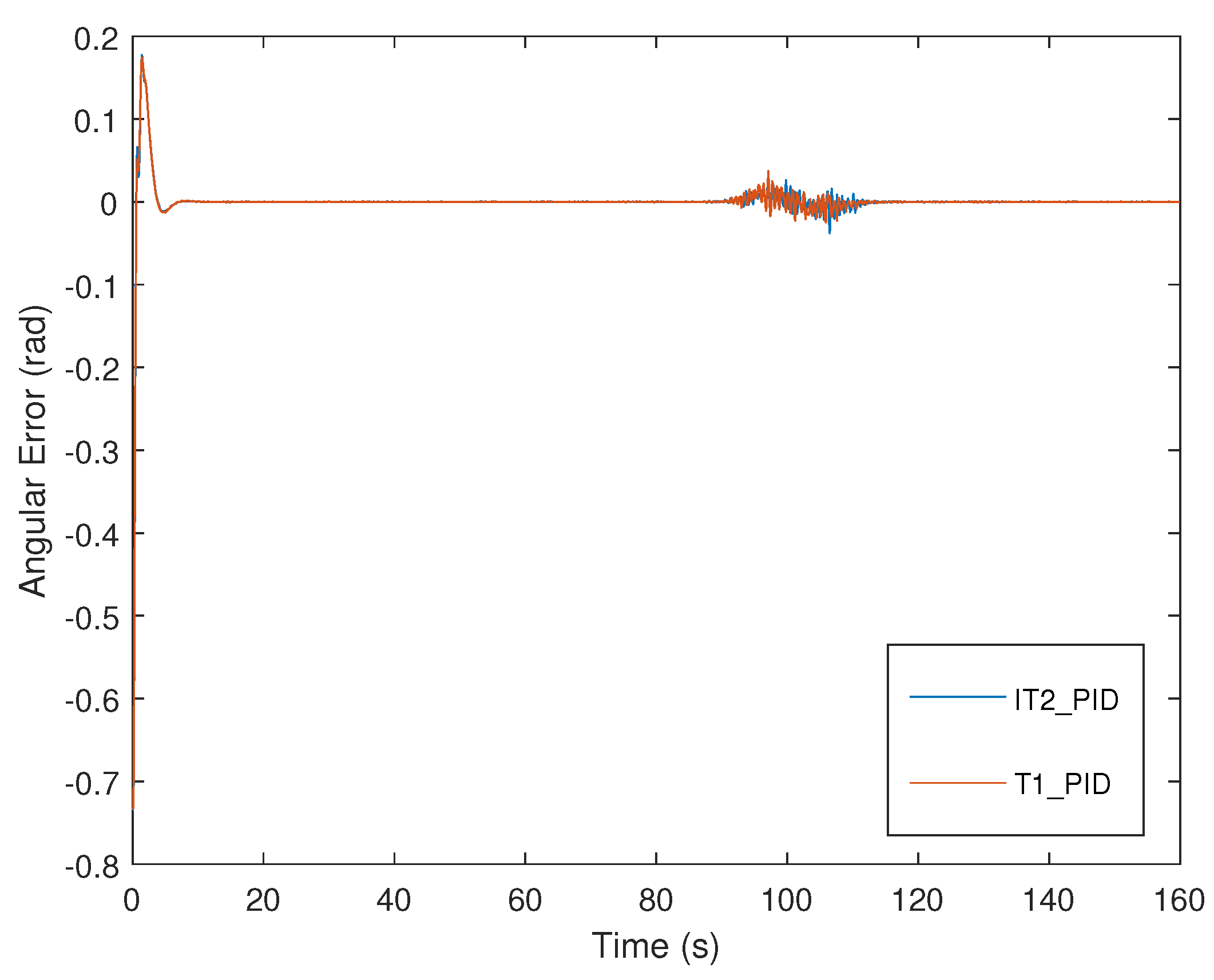
Figure 10, with a forward speed of 0.4 m/s. The mission has a duration of 160 s. At approximately 90 s, the trajectory exhibits an inflection point, at which the line detection and path estimation algorithms display a degree of inaccuracy due to the addition of spurious rectilinear elements. For this experiment, the two fuzzy approaches, IT2_PID and T1_PID, were tested with 50 executions of each controller.
Figure 16 and
Figure 17 display the evolution of the horizontal and angular errors during the mission. It is possible to notice that both controls successfully kept the UAV in the equilibrium condition. At 90 s, the UAV has crossed the point where the trajectory changes direction, which leads to oscillatory behavior in the inferred measurements. Despite this, the UAV remained on the established path throughout the mission.
The numerical results for the IAE are presented in
Table 7. The IT2_PID controller achieved better performance for both the lateral and angular errors. This behavior can be explained by the capability of type-2 fuzzy systems to better cope with uncertainties in the input and output variables of the model [
44].
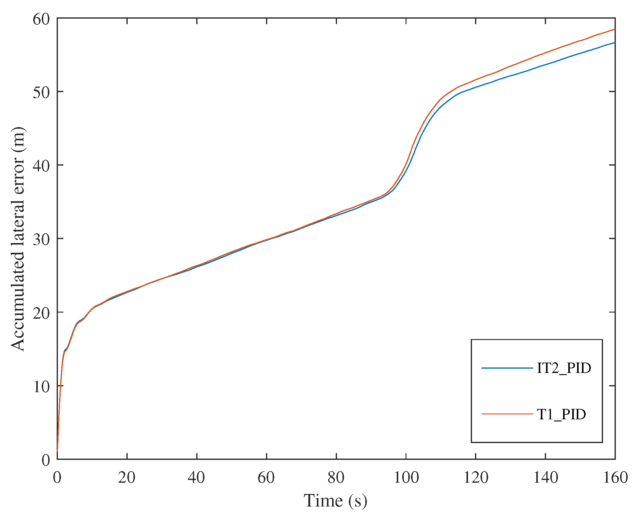
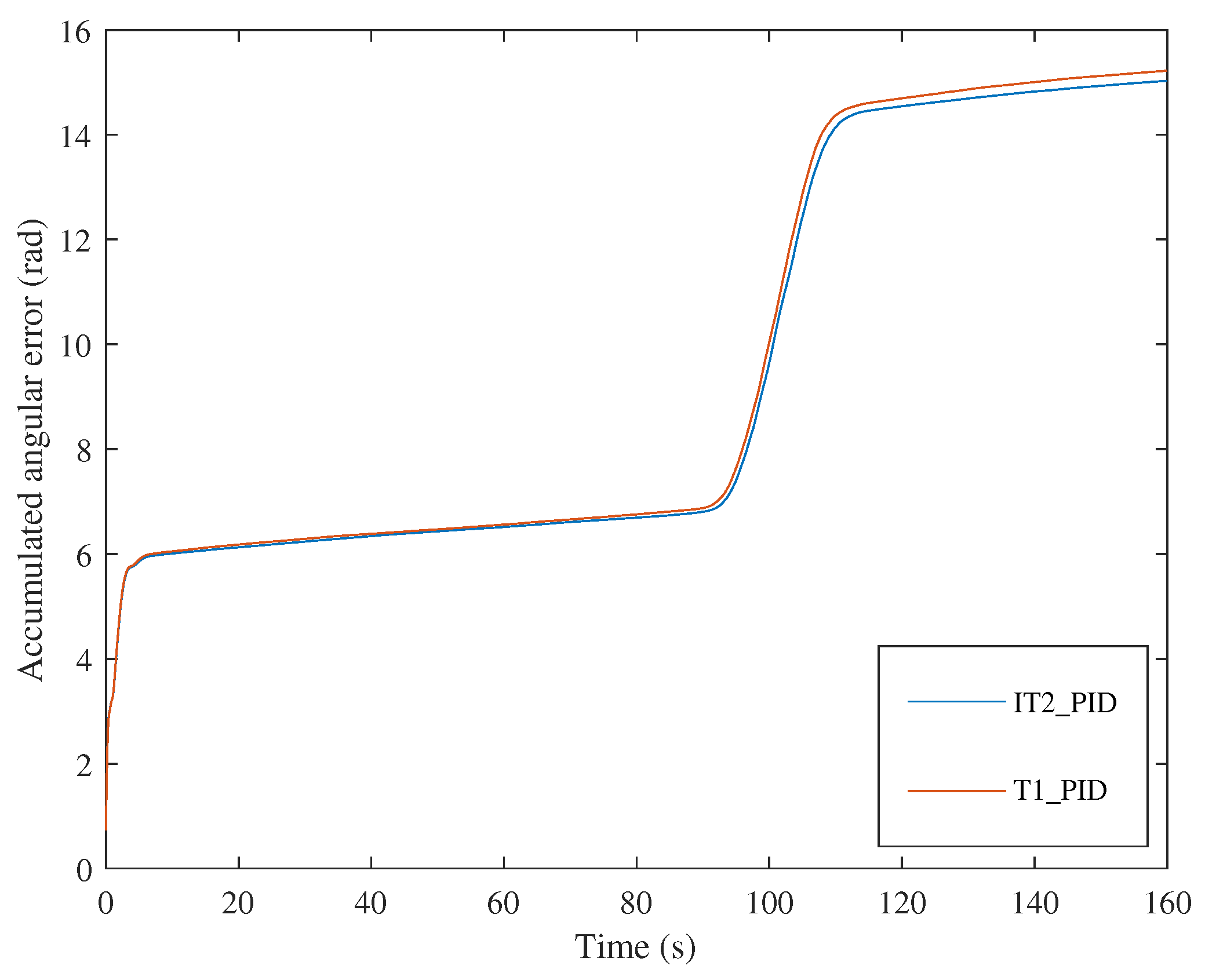
Figure 18 and
Figure 19 present the accumulated errors during the mission. It is possible to notice that the two controllers behave similarly for both variables, with a slight advantage of the IT2_PID controller. When uncertainty is inserted into the model, the difference between the curves becomes more significant for both variables, highlighting the better performance of type-2 fuzzy systems in such scenarios.
3.5. Result Discussions
In the literature, most works involving the use of fuzzy logic as a tuning tool for PID controllers use type-1 fuzzy systems. In this work, however, the use of a type-2 interval fuzzy system was proposed. This modification included an FOU in the membership functions of the model, making it more robust to the effect of noisy data, which is common in robotic systems. The IT2_PID approach showed superior quantitative performance results for the proposed transmission line tracking application over the T1_PID and the classical Ziegler–Nichols tuning method. When comparing the proposed approach with the Ziegler–Nichols method, it was possible to observe reductions in the average values of 29.4% for the IAE, 41.7% in the for the horizontal controller, and 2.47% in the IAE and 58.6% in the for the angular controller. In addition, the settling time was reduced by 51.3% for the horizontal controller and increased by 29.5% for the angle controller.
In the original approach that supported this work, the fuzzy rule set was not modified based on whether the derivative of the error was positive or negative. The authors emphasized this, and thereby a new rule set was introduced in this research to allow the controller to behave more aggressively in situations where the error increases and smooths out otherwise. The results indicated a reduction of 1.9% in the integral of the absolute error and 5.8% for the . It is worth mentioning that further rule combinations can be tested, and this is a topic for future works. Additionally, the rule sets should be evaluated according to the proposed application. Moreover, in order to mitigate the discontinuity behavior brought by fuzzy logic in the control system, the membership functions and rule bases were appropriately designed to ensure smooth transitions between fuzzy sets.
It is also important to highlight that all sensor and actuator integration, image processing, fuzzy logic algorithms, PID controllers, and commands sent to the UAV are handled through the ROS framework in Python scripts, making it possible to test the methodology on several UAV models without the need for significant modifications.
4. Conclusions and Future Work
UAVs have been the focal point of many types of research, expanding the range of possible applications that increasingly support human workers in various tasks. In the scope of power grid maintenance, UAVs can be helpful in the inspection of transmission lines; therefore, algorithms must perform this task as safely and efficiently as possible. With that in mind, the presented work proposed an interval type-2 fuzzy-logic-based PID controller to allow the alignment and tracking of transmission power lines using a UAV.
The algorithm receives the positional and angular errors of the UAV relative to the lines by processed images taken by a camera attached to the aircraft’s base. Next, an interval type-2 fuzzy logic block provides the controller gains based on the errors and their respective derivatives. This approach allows the controller to perform differently based on the magnitude of the input variables. The type-2 fuzzy system introduces a region of uncertainty in these variables, which helps the model deal with noisy data.
The proposed methodology was tested through flights conducted by the Gazebo simulator. For the UAV alignment tests, it can be noticed that the IT2_PID controller achieved superior metrics compared to its T1_PID variant and the traditional Zigler–Nichols tuning technique for both lateral and angular errors, exhibiting lower cumulative error values with lower values. The comparison of the proposed technique with a fixed-gain PID controller based on the average of the fuzzy gain range demonstrated the ability of these models to adapt according to the stage the system is inserted. Experiments involving the following of the UAV through the power lines have shown the capability of the type-2 fuzzy system to better handle the presence of uncertainties in the measurements.
Note that this simulation experiment serves as a prior estimate for the proposed application viability, indicating that the proposed methodology would be feasible to be applied in the proposed scenario. It is also important to highlight that the implemented methodology is thoroughly ready to be tested on a physical PixHawk PX4 FCU due to its robust simulation results and the implemented MavROS ready-to-use offboard controller package. Therefore, testing the developed methodology in a real vehicle is an important next step. However, potential challenges, such as lighting conditions and winds, could harm the process in real applications. In this sense, this work opens several future possibilities. The main point to be addressed is the implementation of the proposed methodology in an embedded system in a real scenario. This task requires robust transmission line detection techniques with a computational effort suitable to the controller requirements in order to mitigate the mentioned issues in a real scenario.
One possible option to be explored for this issue is merging the information acquired by the cameras with laser sensors, allowing for the identification and determination of the distance of the UAV in terms of the power lines to be followed. Another aspect to investigate is the modification of the shape of the membership functions and the effect of the variation in the number of these functions on the controller behavior.

 ,
, 


