A Novel Evolving Type-2 Fuzzy System for Controlling a Mobile Robot under Large Uncertainties

Abstract

This paper presents the development of a type-2 evolving fuzzy control system (T2-EFCS) to facilitate self-learning (either from scratch or from a certain predefined rule). Our system has two major learning stages, namely, structure learning and parameters learning. The structure phase does not require previous information about the fuzzy structure, and it can start the construction of its rules from scratch with only one initial fuzzy rule. The rules are then continuously updated and pruned in an online fashion to achieve the desired set point. For the phase of learning parameters, all adjustable parameters of the fuzzy system are tuned by using a sliding surface method, which is based on the gradient descent algorithm. This method is used to minimize the difference between the expected and actual signals. Our proposed control method is model-free and does not require prior knowledge of the plant’s dynamics or constraints. Instead, data-driven control utilizes artificial intelligence-based techniques, such as fuzzy logic systems, to learn the dynamics of the system and adapt to changes in the system, and account for complex interactions between different components. A robustness term is incorporated into the control effort to deal with external disturbances in the system. The proposed technique is applied to regulate the dynamics of a mobile robot in the presence of multiple external disturbances, demonstrating the robustness of the proposed control systems. A rigorous comparative study with respect to three different controllers is performed, where the outcomes illustrate the superiority of the proposed learning method as evidenced by lower RMSE values and fewer fuzzy parameters. Lastly, stability analysis of the proposed control method is conducted using the Lyapunov stability theory.

1. Introduction

The development of nonlinear control systems for mobile robots has been an important research area in recent years. For example, numerical approaches have been developed for trajectory tracking [1], navigation [2], parking [3], and obstacle avoidance [4]. Traditional control methods have been proposed for tracking control of mobile robots [5] and feedback linearization [6]. Nevertheless, these algorithms can provide satisfactory tracking performance only if the plant’s mathematical model is properly known, which is very difficult in some cases due to various uncertainties (e.g., unmodeled dynamics, and noisy and corrupted measurements) [7].

On the other hand, computational intelligence control approaches, such as fuzzy logic systems (FLSs) and artificial neural networks (ANNs), have lately been applied successfully in trajectory tracking control problems. Intelligent controllers can learn the dynamics of robots in an online manner for both structured and unstructured uncertainties, and also adapt the controller’s parameters and structure based on the operating conditions without the need to obtain a full mathematical model of the plant [7,8].

The flow of work in FLSs is divided into three major steps, namely, fuzzification, the fuzzy inference system (FIS) and defuzzification, respectively. In the first stage, classical or crisp data are transformed into fuzzy data using membership functions, and a degree of confidence is obtained. The degree of confidence in the fuzzy domain is then combined with one of the input features to determine the rule-firing strength. The fuzzy rules follow an if–then structure, with the antecedent being the “if” part and the consequent being the “then” part. Finally, the rule-firing strength is combined with the defuzzification interface to generate the final output [9].

The application of type-1 fuzzy logic control systems (T1-FLCs) has been explored in the context of programming mobile robots to learn and exhibit specific behaviors [10]. However, T1-FLCs have limited ability to handle uncertainties in nonlinear systems, especially in a new operating condition, where the performance degrades significantly [11]. Accordingly, type-2 fuzzy logic control systems (T2-FLCs) and interval type-2 fuzzy logic control systems (IT2-FLCs) can be considered an alternative to solve the limitation of T1-FLCs [12].

IT2-FLCs have been proposed for mobile robot control problems [7,13,14,15], where better tracking performance compared to T1-FLCs were reported. In [4], an interval type-2 fuzzy neural network controller (IT2FNN) was developed for wheeled mobile robot obstacle avoidance. The IT2FNN was compared with its type-1 fuzzy counterpart, where their proposed controller was found to be robust against uncertainties and in the presence of obstacles.

Nevertheless, these conventional IT2-FLCs have a static structure and lack the ability to evolve their structure in an online manner. Generating type-2 fuzzy rules and their associated membership functions is a potential challenge, especially for systems with many variables [16]. Employing evolutionary algorithms to find optimal fuzzy parameters is not desirable due to the large population space which results in slow performance. Hence, the development of an automatic type-2 evolving fuzzy control system (T2-EFCS) is essential to facilitate self-learning (either from scratch or from a certain predefined rule).

Evolving intelligent systems (EISs) are used to describe intelligent systems that can adapt and evolve over time. EISs is a general term that refers to any intelligent system that is capable of evolving over time to improve its performance. EISs can be implemented using various techniques, such as ANNs, and FLSs. The main concept behind EISs is to provide the ability for the system to learn and adapt based on its experiences so that it can improve its performance and become more efficient and effective [17]. On the other hand, evolving fuzzy systems (EFSs) are a specific type of EISs that use FLSs to represent uncertainty and imprecision in the system. EFSs are based on the idea of using fuzzy sets and rules to model the behavior of the system [18].

In [19], EFSs were referred to as Smart Adaptive Systems, where they differ from adaptive systems and have the following features: (1) autonomous systems, where they are able to evolve on their own; (2) flexible to change, where they are able to simultaneously evolve both their structure and parameters; (3) able to respond to a surprise (e.g., unexpected inputs); (4) able to accumulate experience (e.g., able to build-up their architecture during the routine process); and (5) smart (able to make decisions).

There is a strong correlation between EISs and EFSs, as both concepts are focused on developing intelligent systems that can adapt and evolve over time. However, EFSs are more specific in that they use FLSs to represent uncertainty and imprecision in nonlinear systems, while EISs, on the other hand, is a more general term that can refer to any type of intelligent system that can evolve over time. Recently, evolving fuzzy systems have become popular in various engineering applications. They are used for system identification, regression, classification, and control [20,21].

EISs was first conceptualized in [22] for single-pass incremental learning, with self-constructing neural fuzzy inference network (SONFIN) capabilities. SONFIN can learn both structure and parameters in an online manner. Nevertheless, it cannot remove ineffective rules. Kasabov and Song [23] proposed a new technique named a dynamic evolving neural fuzzy inference system (DENFIS) based on the evolving clustering method (ECM), where ECM requires a threshold value for defining the maximum distance between each data sampleand cluster centers. Angelov and Filev [24] developed an evolving Takagi–Sugeno (eTS) fuzzy system that can evolve its structure from scratch without any prior knowledge of the system. However, their proposed algorithm is not capable of eliminating redundant fuzzy rules. In [25], a sequential adaptive fuzzy inference system (SAFIS) was proposed, where the Kalman filter is utilized for updating the parameters. Angelov [26] developed a new version of eTS called eTS+, where the online dimensionality was reduced compared to the original eTS. In [27], a parsimonious network based on a fuzzy inference system (PANFIS) was developed as an improved version of SAFIS, where the extended recursive least square method was utilized to guarantee the stability of the learning algorithms.

In the control systems domain, EFSs have been used to control nonlinear systems. In [28], a generic self-evolving neuro-fuzzy controller was designed for trajectory tracking of bio-inspired unmanned aerial vehicles and also to achieve a robust control performance of a voice coil motor in [29]. These recent controllers learned their structure from scratch and utilized the sliding mode theory for adapting fuzzy parameters. In another study in [30], a self-evolving fuzzy controller was designed for a hypersonic vehicle with online structure and parameter learning. Their simulation results demonstrated superior performance over a fixed-structure fuzzy system. However, their proposed controller was model based, requiring an accurate mathematical model of the system. Furthermore, most of the real-world applications are nonlinear, making it difficult to establish an accurate mathematical model, especially in the presence of external disturbances and other types of uncertainties; hence, it is important to design a model-free controller, which does not require knowledge of the plant dynamics.

The integration of EFSs and type-2 fuzzy logic systems was first introduced by Juang and Tsao [31], with an improvement over their proposed SONFIN using the evolving structure. In [31], a self-evolving fuzzy logic system was developed to generate fuzzy rules from scratch for modeling nonlinear systems. Their proposed algorithm utilized the Kalman filter for parameter learning of the consequent part, while the antecedent part was learned by the gradient descent method. The same algorithm was implemented in [32] for the system identification of nonlinear systems. In [33,34], fuzzy rules were generated from input–output data, and the entropy criterion was used to determine when to extract and generate a new fuzzy rule. However, one drawback of this framework is that once the rule is created, it cannot be pruned. Hence, several pruning techniques were proposed in the literature to reduce the complexity of rule base design and improve the readability and interpretability of rule semantics [35].

Evolving type-2 fuzzy logic systems were utilized to control nonlinear systems. In [36], a function-link self-evolving type-2 fuzzy system was proposed for nonlinear system identification and control, where good results were obtained using their proposed method. Another self-adaptive type-2 fuzzy controller [37] was proposed to control permanent magnet linear synchronous motor (PMLSM) drivers. Nevertheless, the actual system is still assisted by a proportional-derivative (PD) controller.

A particle swarm optimization technique was used to find the optimal learning rates in [38] to construct their proposed interval type-2 fuzzy brain emotional learning control system. However, the efficacy of their proposed approaches in the face of various uncertainties has not been investigated adequately.

To accommodate more uncertainties in capturing the dynamics of nonlinear systems and to design a self-sufficient controller, the contributions of this paper can be summarized as follows:

• A novel type-2 evolving fuzzy control system (T2-EFCS) supported by efficient pruning rules is introduced. The adaptive law is derived using the sliding mode control (SMC) theory to guarantee the systems’ robustness against uncertainties.
• The proposed closed-loop control system is employed to control a simulated mobile robot, where the robustness is investigated in the presence of external disturbance (e.g., noisy sensor measurements). For disturbance rejection, a new robustness term is added to obtain robust control performance against uncertainties.
• A rigorous comparative study with respect to three different controllers, such as T1-FLC, T2-FLC, and T1-EFCS, is performed, where the outcomes of this study illustrate the superiority of the proposed method with lower RMSE values.
• The stability analysis of the proposed method is implemented using the Lyapunov stability theory.

The remainder of this paper is structured as follows. The problem formulation is discussed in Section 2. The T2-EFCS control system design is presented in Section 3, including the adding mechanism, the pruning mechanism, and the parameter adaptation of type-2 fuzzy rules. Section 4 describes the stability proof of our proposed T2-EFCS. The system description of a mobile robot is provided in Section 5. The simulation results are discussed in Section 6. Finally, Section 7 provides a concluding remark of this paper.

2. Problem Formulation

A class of a n-th order nonlinear dynamic system can be described as follows:

$$\left\{\begin{array}{c}{x}^{\left(n\right)}=\underline{f}\left(\underline{x}\right)+\underline{b}\left(\underline{x}\right)u+d\left(\underline{x}\right)\hfill \\ y=x,\hfill \end{array}\right.$$

(1)

where the state vector $\underline{x}\in {\Re }^m$ can be defined as $\underline{\mathbf{x}}={\left[\begin{array}{cccc}x& \dot{x}& \dots & x^{(n-1)}\end{array}\right]}^T\in {\Re }^m$; $x\in {\Re }^m$ represents the state; $\underline{f}\left(\underline{x}\right)\in {\Re }^m$ and $\underline{b}\left(\underline{x}\right)\in {\Re }^{m\times m}$ are the system nonlinear functions; u depicts the control input; y is the system output; and $d\left(\underline{x}\right)\in {\Re }^m$ expresses unknown uncertainties. For the theoretical study, it is assumed that the nonlinear terms in (1) are known and bounded, and ${\underline{b}}^{-1}\left(\underline{x}\right)$ exists for all x.

Assumption 1.

If there existinevitable modeling uncertainties between the real system and the simulated systems, they can be absorbed in the uncertainty function.

The purpose of the closed-loop control system is that the system output y has the ability to track a desired signal $y_d$. Consider the tracking error as

$$e=y_d-y,$$

(2)

and the system tracking vector can be written as

$$\underline{e}={\left[\begin{array}{cccc}e\left(t\right)& \dot{e}\left(t\right)& \dots & e{\left(t\right)}^{(n-1)}\end{array}\right]}^T\in {\Re }^{nm}.$$

(3)

Define an integrated sliding surface as

$$S_{EFC}\equiv e^{n-1}+{\kappa }_1{e}^{n-2}+\dots +{\kappa }_n{\int }_0^{t}e\left(\tau \right)d\tau ,$$

(4)

where ${\kappa }_i\in {\Re }^{m\times m}$ is a strictly positive constant matrix, where $i=1,2,3\dots ,n$; and $\kappa ={\left[{\kappa }_1,\dots ,{\kappa }_n\right]}^T\in {\Re }^{nm\times m}$. If the nonlinear terms $\underline{f}\left(\underline{x}\right)$ and $\underline{b}\left(\underline{x}\right)$ and also the $d\left(\underline{x}\right)$ are known, an ideal control law $u_{fin}\left(t\right)$ can be designed as follows [36,38,39]:

$$u_{fin}=\underline{b}\left(\underline{x}\right){}^{-1}\left[y_d^{\left(n\right)}-\underline{f}\left(\underline{x}\right)-d\left(\underline{x}\right)+{\kappa }^T\underline{e}\right].$$

(5)

Using (5) and (1), we can derive the following error dynamic equation as:

$${\dot{S}}_{EFC}=e^{\left(n\right)}+{\kappa }^T\underline{e}=0$$

(6)

From (6), it is clear that if $\kappa$ is chosen to correspond to the Hurwitz polynomial coefficients, it leads to a convergence of the tracking error to zero when the time approaches infinity [39]. Nevertheless, in real-time applications, the uncertainty term $d\left(\underline{x}\right)$ cannot be precisely known. Therefore, the ideal control law in (5) is not available.

For this study, we assume there is an optimal T2-EFCS controller $u_{T2-EFCS}^{*}$ to approximate the ideal controller $u_{fin}$ in (5), where $u_{T2-EFCS}^{*}$ is function of $\left({\overline{m}}^{*},{\underline{m}}^{*},{\sigma }^{*},W^{*},t\right)$ so that $u_{fin}=u_{T2-EFCS}^{*}\left({\overline{m}}^{*},{\underline{m}}^{*},{\sigma }^{*},W^{*},t\right)+\epsilon \left(t\right)$, where ${\overline{m}}^{*},{\underline{m}}^{*},{\sigma }^{*},W^{*},t$ are the optimal parameters for $\overline{m},\underline{m},\sigma ,W$ and $\epsilon \left(t\right)$ is the approximation error. As we cannot obtain the optimal parameters accurately, the estimation control system is utilized as follows [40]:

$${\widehat{u}}_{fin}={\widehat{u}}_{T2-EFCS}\left(\widehat{\overline{m}},\widehat{\underline{m}},\widehat{\sigma },\widehat{W},t\right)$$

(7)

where $\widehat{\overline{m}},\widehat{\underline{m}},\widehat{\sigma },\widehat{W}$ are the estimation of the optimal parameters. The robustness term is discussed in Section 3.4.

3. T2-EFCS Control System Design

3.1. T2-EFCS Architecture

The structure of the proposed evolving interval type-2 fuzzy control system is discussed in this section. It consists of five layers, namely, the input layer, the fuzzification layer, the firing strength layer, the consequent layer, and the output layer. Each rule has the following form:

$$\begin{array}{c}\hfill RUL{E}^m:If(x_{1}is{\tilde{X}}_1^m,x_{2}is{\tilde{X}}_2^m,\dots ,x_{n}is{\tilde{X}}_n^m),\\ \hfill THEN{\tilde{y}}_m=\sum _{n=1}^M{W}_m^n\left(t\right)x_n\left(t\right),\end{array}$$

where $x=x_1,\dots ,x_n$ denotes the inputs variables to T2-EFCS, $m=1,2,\dots ,M$, where M represents the number of fuzzy rules, $W_m^n\in {\Re }^M$ denotes the weight vector of the fuzzy logic consequent part, and ${\tilde{X}}_n^m$ and $\tilde{y}$ are the interval type-2 fuzzy membership functions for the input and output, respectively. Each layer can be described as follows:

• Layer 1 (Input layer): This layer is the input signals with $(n\times 1)$ vector. In this study, the error and its derivative are the two inputs to the system.
• Layer 2 (Fuzzification layer): This layer is the first hidden layer, which can be expressed by IT2 membership functions. In this study, a Gaussian membership function with fixed width ${\sigma }_n^m$ and uncertain means $\left[{\overline{m}}_{mn},{\underline{m}}_{mn}\right]$ is deployed as shown in Figure 1, which can be given as follows [41]:

  $${\overline{\mu }}_{mn}=exp\left\{-\frac{1}{2}{\left(\frac{x_n-{\overline{m}}_{mn}}{{\sigma }_{mn}}\right)}^2\right\},$$

  (8)

  $${\underline{\mu }}_{mn}=exp\left\{-\frac{1}{2}{\left(\frac{x_n-{\underline{m}}_{mn}}{{\sigma }_{mn}}\right)}^2\right\}.$$

  (9)
• Layer 3 (Firing layer): The firing strength $F_m$ is computed in this layer to perform the aggregation operation:

  $$F_m=[{\underline{f}}_m,{\overline{f}}_m],$$

  (10)

  where

  $$\left\{\begin{array}{c}\hfill {\underline{f}}_m=\prod _{n=1}^p{\underline{\mu }}_{mn}\hfill \\ \hfill {\overline{f}}_m=\prod _{n=1}^p{\overline{\mu }}_{mn}.\hfill \end{array}\right.$$
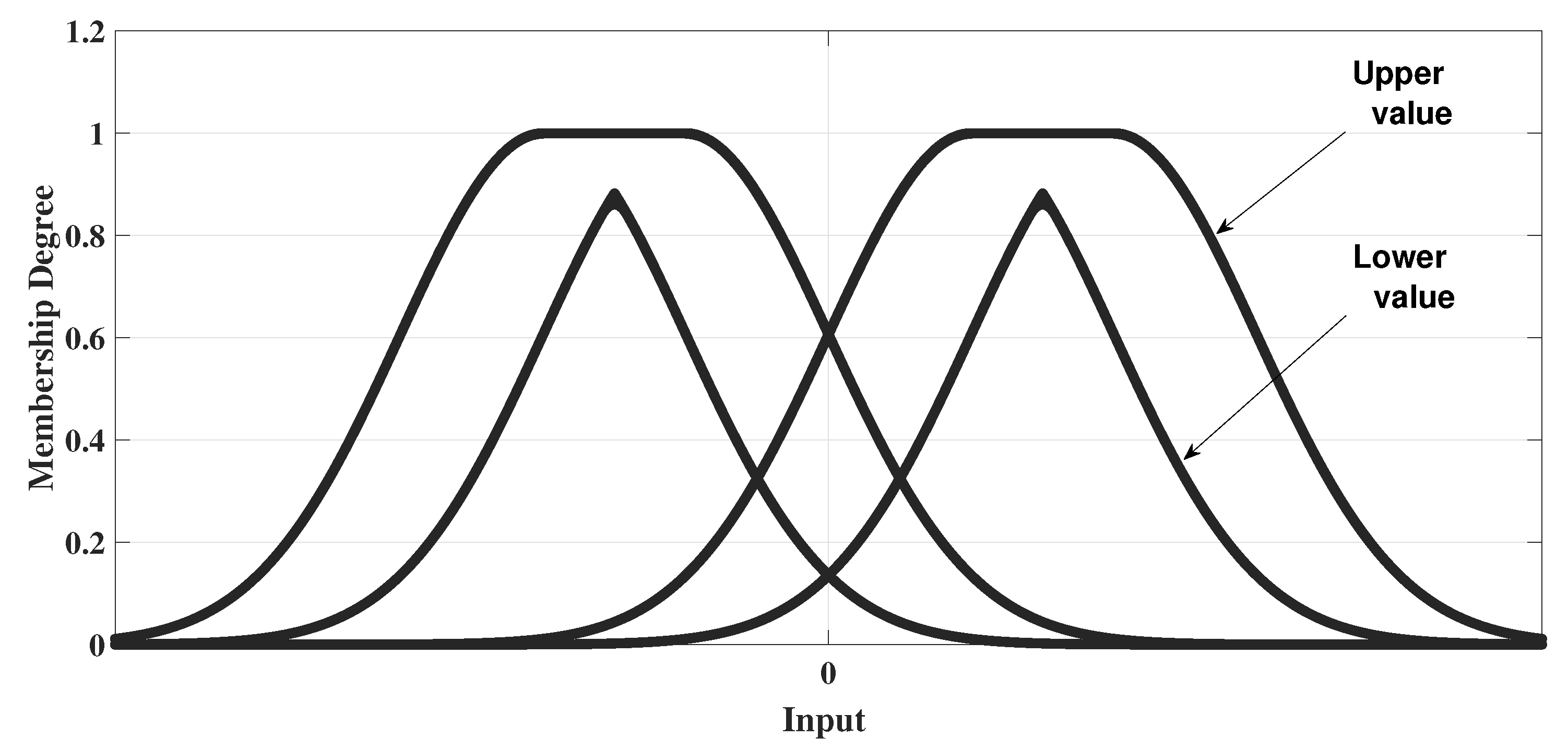
• Layer 4 (Consequent layer): the output of this layer has two consequent values as follows:

  $$\left\{\begin{array}{c}\hfill \underline{y}\left(t\right)={\displaystyle \frac{{\sum }_{m=1}^M{\underline{f}}_m\left(t\right)y_m\left(t\right)}{{\sum }_{n=1}^M{\underline{f}}_m\left(t\right)}}\hfill \\ \hfill \overline{y}\left(t\right)={\displaystyle \frac{{\sum }_{m=1}^M{\overline{f}}_m\left(t\right)y_m\left(t\right)}{{\sum }_{m=1}^M{\overline{f}}_m\left(t\right)}},\hfill \end{array}\right.$$

  (11)

  where $\overline{y}\left(t\right)$ and $\underline{y}\left(t\right)$ are the upper and lower outputs of the consequent part, respectively. In this layer, the center-of-sets and the ‘Enhanced Iterative Algorithm with Stop Condition’ type-reducer were utilized to calculate the interval outputs $[\overline{y}\left(t\right),\underline{y}\left(t\right)]$.
• Layer 5 (Output layer): The computation of the output value of the last layer is given as follows:

  $$y=\varrho \overline{y}\left(t\right)+(1-\varrho )\underline{y}\left(t\right),$$

  (12)

  where $\varrho \in [0,0.5]$ represents a weighting parameter.

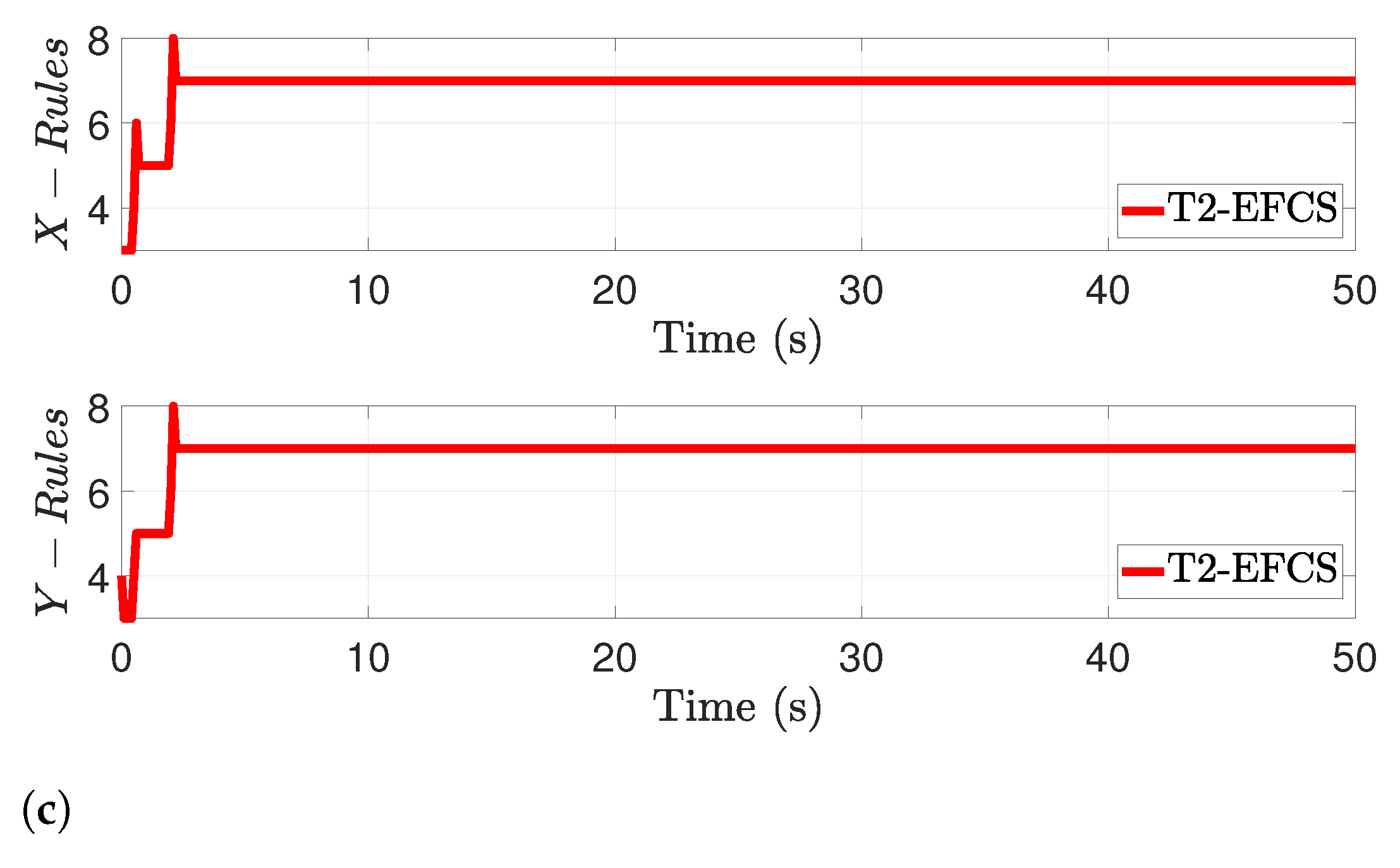
3.2. T2-EFCS Structure Learning

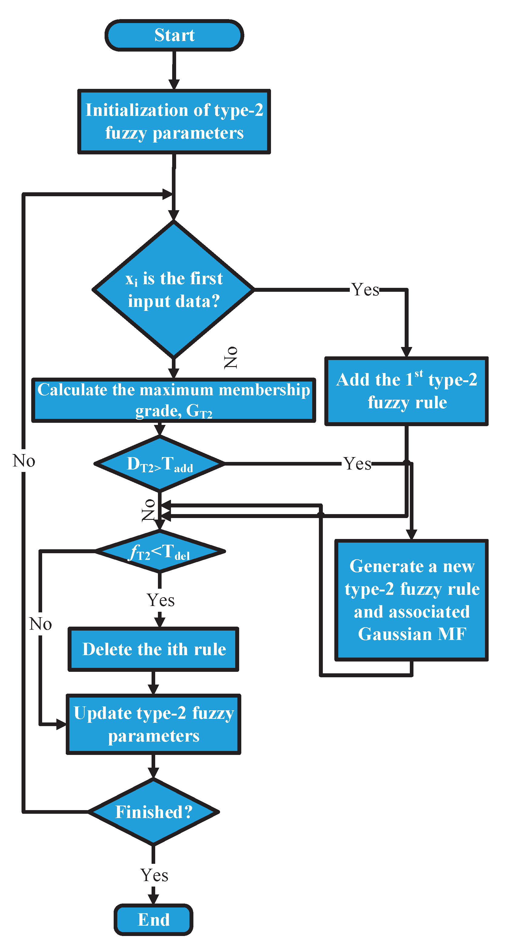
• Rule-Adding Mechanism: The rule generation of T2-EFCS is based on the distance between the incoming data and the upper and lower means of the type-2 Gaussian function so that when $max{D}_{T2}>T_{add}$, a new rule is generated. The Euclidean distance of the upper and lower means can be computed using the following equation:

  $$\begin{array}{ccc}D(x_n,m_M)& =& \Vert x_n-m_M{\Vert }_2\end{array},$$

  (13)

  where $x_n$ represents the incoming data of e and $\dot{e}$; $m_M=\left(({\overline{m}}_M+{\underline{m}}_M)/2\right)$ is the mean. If we define a MAX-MIN approach to identify when to add a new type-2 fuzzy rule as, $\widehat{M}=arg\underset{1\le M\le n_M}{min}D(x_n,m_M)$, the T2-EFCS finds

  $$\begin{array}{c}\hfill \mathit{If}(\max D_{T2}>T_{add})\mathrm{THEN}\\ \hfill \mathit{Generate}\mathrm{new}\mathrm{type}-2\mathrm{fuzzy}\mathrm{rule}\end{array}$$

  where $T_{add}$ denotes a prior threshold value for rule generation.
  The initial type-2 fuzzy MF parameters are set as

  $$\left\{\begin{array}{cc}\left[m_{1n}^1,m_{1n}^2\right]\hfill & =\left[x_n-\mathsf{\Delta }x,x_n+\mathsf{\Delta }x\right]\hfill \\ \sigma \hfill & ={\sigma }_{fixed}\hfill \end{array}\right.$$

  (14)

  where ${\sigma }_{fixed}$ denotes a predefined value (in this work, ${\sigma }_{fixed}=0.5$), which determines the width of the membership functions associated with a newly generated rule, $m_{1n}^1$ and $m_{1n}^2$ are the uncertain center of the membership function associated with a newly generated rule, and $\mathsf{\Delta }x$ is the width of uncertain region.
  Once a new type-2 fuzzy rule is generated, the same procedure implemented for the first rule is utilized to assign the uncertain mean and the width as follows:

  $$\left\{\begin{array}{cc}\left[m_{1n}^{M\left(t\right)+1},m_{1n}^{M\left(t\right)+2}\right]\hfill & =\left[x_n-\mathsf{\Delta }x,x_n+\mathsf{\Delta }x\right]\hfill \\ {\sigma }^{M\left(t\right)+1}\hfill & =\xi .\left|x_n-\left(\frac{m_{12}^I+m_{12}^I}{2}\right)\right|\hfill \end{array}\right.$$

  (15)

  where $\xi$ represents an overlapping parameter ($\xi$ is set to $0.5$ in this work), and $M\left(t\right)$ represents the total number of type-2 fuzzy rules at the $t^{th}$ step.

Remark 1.

If the uncertainty associated with the mean $\mathsf{\Delta }x$ is very small, the type-2 GF becomes similar to the type-1 GF. Nevertheless, if the uncertain region of type-2 GF with is extremely large, it covers all input domains, where a lower number of rules is generated [36,42].

• Rule Pruning Mechanism: In this proposed technique, deleting unnecessary rules is considered. The process of pruning existing rules is based on the contribution of membership grade, so when it is smaller than the prior threshold value, the rule is deleted. This approach can be expressed as follows:

  $$\mathit{If}(F_m<T_{del})\mathit{THEN}\mathrm{delete}\mathrm{type}-2ith\mathrm{fuzzy}\mathrm{rule}$$

  where $T_{del}$ denotes a prior threshold value for rule deletion, and $F_{T2}=F_m$, which denotes the firing strength in (10) for each incoming data.
  Automatic rules generation and pruning are efficient, which determine the optimal number of fuzzy rules. Figure 2 illustrates the flowchart of the proposed method. The online update of type-2 fuzzy parameters is presented in the following section.

Remark 2.

The selection of the adding/pruning threshold parameters $T_{add}$ and $T_{del}$ is based on the maximum number of fuzzy rules (MNFR), where MNFR is a design parameter that determines the maximum number of fuzzy rules when a fuzzy structure evolves. These threshold values are confined in (0,1). The empirical relationship between the adding/pruning thresholds values ($T_{add}$, $T_{del}$) and MNFR is described as $[T_{add}\ge (1/MNFR)]$ and $[T_{del}\ge (1/MNFR)]$. This way, the parameters of the T2-EFCS are meaningful to the user. For instance, if MNFR is selected to be 7, then $T_{add}$ and $T_{del}$ should be selected ≥ 0.143. If MNFR is selected to be 15, then $T_{add}$ and $T_{del}$ should be ≥ 0.067. Higher MNFR values result in higher accuracy, but also higher processing time. The selection of MNFR is a trade-off between the processing unit capabilities and controllers’ accuracy [43].

3.3. T2-EFCS Parameters Learning

The gradient descent method is applied to minimize the error function between the desired and the actual output. Sliding mode control is utilized to optimize the upper and lower parameters of our proposed T2-EFCS system using a self-tuning technique, making the system robust to variations in system parameters and external disturbance [14]. The online adaptation law of the proposed T2-EFCS is given in the following equations as [36,38]:

$${\widehat{\overline{m}}}_{mn}(t+1)={\widehat{\overline{m}}}_{mn}\left(t\right)-{\widehat{\eta }}_m\frac{\partial s_{EFC}\left(t\right){\dot{s}}_{EFC}\left(t\right)}{\partial {\widehat{\overline{m}}}_{mn}}$$

(16)

$${\widehat{\underline{m}}}_{mn}(t+1)={\widehat{\underline{m}}}_{mn}\left(t\right)-{\widehat{\eta }}_m\frac{\partial s_{EFC}\left(t\right){\dot{s}}_{EFC}\left(t\right)}{\partial {\widehat{\underline{m}}}_{mn}}$$

(17)

$${\widehat{\sigma }}_{mn}(t+1)={\widehat{\sigma }}_{mn}\left(t\right)-{\widehat{\eta }}_{\sigma }\frac{\partial s_{EFC}\left(t\right){\dot{s}}_{EFC}\left(t\right)}{\partial {\widehat{\sigma }}_{mn}}$$

(18)

$${\widehat{W}}_{nk}(t+1)={\widehat{W}}_{nk}\left(t\right)-{\widehat{\eta }}_W\frac{\partial s_{EFC}\left(t\right){\dot{s}}_{EFC}\left(t\right)}{\partial {\widehat{W}}_{nk}}$$

(19)

where ${\widehat{\eta }}_m$, ${\widehat{\eta }}_{\sigma }$, and ${\widehat{\eta }}_W$ are the learning rates to update T2-EFCS parameters.

By applying the chain rule, the following equations can be derived:

$$\begin{array}{ccc}\frac{\partial s_{EFC}\left(t\right){\dot{s}}_{EFC}\left(t\right)}{\partial {\widehat{\overline{m}}}_{mn}}& =& \frac{1}{2}\frac{\partial s_{EFC}\left(t\right){\dot{s}}_{EFC}\left(t\right)}{\partial {\widehat{u}}_{T2-EFCS}}\left(\frac{\partial \underline{y}}{\partial {\underline{f}}_m}\frac{\partial {\underline{f}}_m}{\partial {\widehat{\overline{m}}}_{mn}}+\frac{\partial \overline{y}}{\partial {\overline{f}}_m}\frac{\partial {\overline{f}}_m}{\partial {\widehat{\overline{m}}}_{mn}}\right)\\ & =& \frac{1}{2}{s}_{EFC}\left(t\right)\left(\frac{\left(w_m-\underline{y}\right)}{{\sum }_{m=1}^M{\underline{f}}_m}\frac{\partial {\underline{f}}_m}{\partial {\widehat{\overline{m}}}_{mn}}+\frac{\left(w_m-\overline{y}\right)}{{\sum }_{m=1}^M{\overline{f}}_m}\frac{\partial {\overline{f}}_m}{\partial {\widehat{\overline{m}}}_{mn}}\right)\end{array}$$

(20)

$$\begin{array}{ccc}\frac{\partial s_{EFC}\left(t\right){\dot{s}}_{EFC}\left(t\right)}{\partial {\widehat{\underline{m}}}_{mn}}& =& \frac{1}{2}\frac{\partial s_{EFC}\left(t\right){\dot{s}}_{EFC}\left(t\right)}{\partial {\widehat{u}}_{T2-EFCS}}\left(\frac{\partial \underline{y}}{\partial {\underline{f}}_m}\frac{\partial {\underline{f}}_m}{\partial {\widehat{\underline{m}}}_{mn}}+\frac{\partial \overline{y}}{\partial {\overline{f}}_m}\frac{\partial {\overline{f}}_m}{\partial {\widehat{\underline{m}}}_{mn}}\right)\\ & =& \frac{1}{2}{s}_{EFC}\left(t\right)\left(\frac{\left(w_m-\underline{y}\right)}{{\sum }_{m=1}^M{\underline{f}}_m}\frac{\partial {\underline{f}}_m}{\partial {\widehat{\underline{m}}}_{mn}}+\frac{\left(w_m-\overline{y}\right)}{{\sum }_{m=1}^M{\overline{f}}_m}\frac{\partial {\overline{f}}_m}{\partial {\widehat{\underline{m}}}_{mn}}\right)\end{array}$$

(21)

$$\begin{array}{ccc}\frac{\partial s_{EFC}\left(t\right){\dot{s}}_{EFC}\left(t\right)}{\partial {\widehat{\sigma }}_{mn}}& =& \frac{1}{2}\frac{\partial s_{EFC}\left(t\right){\dot{s}}_{EFC}\left(t\right)}{\partial {\widehat{u}}_{T2-EFCS}}\left(\frac{\partial \underline{y}}{\partial {\underline{f}}_m}\frac{\partial {\underline{f}}_m}{\partial \widehat{\sigma }}+\frac{\partial \overline{y}}{\partial {\overline{f}}_m}\frac{\partial {\overline{f}}_m}{\partial \widehat{\sigma }}\right)\\ & =& \frac{1}{2}{s}_{EFC}\left(t\right)\left(\frac{\left(w_m-\underline{y}\right)}{{\sum }_{m=1}^M{\underline{f}}_m}\frac{\partial {\underline{f}}_m}{\partial \widehat{\sigma }}+\frac{\left(w_m-\overline{y}\right)}{{\sum }_{m=1}^M{\overline{f}}_m}\frac{\partial {\overline{f}}_m}{\partial \widehat{\sigma }}\right)\end{array}$$

(22)

$$\begin{array}{ccc}\frac{\partial s_{EFC}\left(t\right){\dot{s}}_{EFC}\left(t\right)}{\partial {\widehat{W}}_{nk}}& =& \frac{1}{2}\frac{\partial s_{EFC}\left(t\right){\dot{s}}_{EFC}\left(t\right)}{\partial {\widehat{u}}_{T2-EFCS}}\frac{\partial {\widehat{u}}_{T2-EFCS}}{\partial y}\frac{\partial y}{\partial W}\\ & =& \frac{1}{2}{s}_{EFC}\left(t\right)\left(\frac{{\underline{f}}_m}{{\sum }_{m=1}^M{\underline{f}}_m}+\frac{{\overline{f}}_m}{{\sum }_{m=1}^M{\overline{f}}_m}\right)\end{array}$$

(23)

From (10), the following can be derived:

$$\begin{array}{ccccc}\frac{\partial {\underline{f}}_m}{\partial {\widehat{\overline{m}}}_{mn}}& =& \frac{\partial {\underline{f}}_m}{\partial {\underline{\mu }}_{mn}}\frac{\partial {\underline{\mu }}_{mn}}{\partial {\widehat{\overline{m}}}_{mn}}& ={\underline{f}}_m& \frac{{\left(x_n-{\widehat{\overline{m}}}_{mn}\right)}^2}{{\left({\widehat{\sigma }}_{mn}\right)}^3}\\ \frac{\partial {\overline{f}}_m}{\partial {\widehat{\overline{m}}}_{mn}}& =& \frac{\partial {\overline{f}}_m}{{\overline{\mu }}_{mn}}\frac{{\overline{\mu }}_{mn}}{\partial {\widehat{\overline{m}}}_{mn}}& ={\overline{f}}_m& \frac{{\left(x_n-{\widehat{\overline{m}}}_{mn}\right)}^2}{{\left({\widehat{\sigma }}_{mn}\right)}^3}\\ \frac{\partial {\underline{f}}_m}{\partial {\widehat{\underline{m}}}_{mn}}& =& \frac{\partial {\underline{f}}_m}{\partial {\underline{\mu }}_{mn}}\frac{\partial {\underline{\mu }}_{mn}}{\partial {\widehat{\underline{m}}}_{mn}}& ={\underline{f}}_m& \frac{{\left(x_n-{\widehat{\underline{m}}}_{mn}\right)}^2}{{\left({\widehat{\sigma }}_{mn}\right)}^3}\\ \frac{\partial {\overline{f}}_m}{\partial {\widehat{\underline{m}}}_{mn}}& =& \frac{\partial {\overline{f}}_m}{{\overline{\mu }}_{mn}}\frac{{\overline{\mu }}_{mn}}{\partial {\widehat{\underline{m}}}_{mn}}& ={\overline{f}}_m& \frac{{\left(x_n-{\widehat{\underline{m}}}_{mn}\right)}^2}{{\left({\widehat{\sigma }}_{mn}\right)}^3}\\ \frac{\partial {\underline{f}}_m}{\partial \widehat{{\sigma }_{mn}}}& =& \frac{\partial {\underline{f}}_m}{\partial {\underline{\mu }}_{mn}}\frac{\partial {\underline{\mu }}_{mn}}{\partial \widehat{\sigma }}& ={\underline{f}}_m& \frac{{\left(x_n-{\widehat{\underline{m}}}_{mn}\right)}^2}{{\left({\widehat{\sigma }}_{mn}\right)}^3}\\ \frac{\partial {\overline{f}}_m}{\partial {\widehat{\sigma }}_{mn}}& =& \frac{\partial {\overline{f}}_m}{\partial {\overline{\mu }}_{mn}}\frac{{\overline{\mu }}_{mn}}{\partial \widehat{\sigma }}& ={\overline{f}}_m& \frac{{\left(x_n-{\widehat{\overline{m}}}_{mn}\right)}^2}{{\left({\widehat{\sigma }}_{mn}\right)}^3}\end{array}$$

(24)

3.4. T2-EFCS Robustness Term

For obtaining a robust control performance in the face of uncertainties, a disturbance elimination term, $u_{robust}$, is added to the final control input. Therefore, the final control input can be expressed as

$${\widehat{u}}_{fin}={\widehat{u}}_{T2-EFCS}\left(\widehat{\overline{m}},\widehat{\underline{m}},\widehat{\sigma },\widehat{W},t\right)+{\widehat{u}}_{robust}$$

(25)

where ${\widehat{u}}_{robust}$ is a robustifying term [43,44], which can be represented as follows:

$${\widehat{u}}_{robust}=\beta sat\left(S_{EFC}\left(t\right)\right),$$

(26)

where $\beta$ denotes a design parameter, and $sat$ can be defined as follows:

$$sat\left(\frac{S_{EFC}}{\iota }\right)=\left\{\begin{array}{cc}\frac{S_{EFC}}{\iota },\hfill & if\left|S_{EFC}\right|\le \left|\iota \right|\hfill \\ sgn\left(S_{EFC}\right),\hfill & otherwise\hfill \end{array}\right.$$

(27)

where $\iota$ is a design factor representing the thickness of the boundary layer. The $sgn$ represents the $signum$ function, which can be defined as follows:

$$sgn\left(S_{EFC}\left(t\right)\right)=\left\{\begin{array}{cc}\hfill 1,\hfill & \hfill if{S}_{EFC}\left(t\right)>0\hfill \\ \hfill 0,\hfill & \hfill if{S}_{EFC}\left(t\right)=0\hfill \\ \hfill -1,\hfill & \hfill if{S}_{EFC}\left(t\right)<0\hfill \end{array}\right.$$

(28)

4. T2-EFCS Stability Proof

The Lyapunov function is defined as [36,38]:

$$V\left(s_{EFC}\left(t\right)\right)=\frac{1}{2}{s}_{EFC}^2\left(t\right)$$

(29)

$$\dot{V}\left(s_{EFC}\left(t\right)\right)=s_{EFC}\left(t\right){\dot{s}}_{EFC}\left(t\right)$$

(30)

Following the derivation on [36], one can introduce a matrix such that $Q_{\mathcal{O}}\left(t\right)=\frac{\partial {\widehat{u}}_{T2-EFCS}}{\partial O},$ for $O=\widehat{\underline{m}},\widehat{\overline{m}},\widehat{\sigma },\widehat{W}$ where

$$\begin{array}{cc}\hfill Q_{\widehat{\underline{m}}}\left(t\right)=\frac{\partial {\widehat{u}}_{T2-EFCS}}{\partial \widehat{\underline{m}}}& \hfill =\left[\frac{\partial {\widehat{u}}_{T2-EFCS}}{\partial {\widehat{\underline{m}}}_{11}},\dots ,\frac{\partial {\widehat{u}}_{T2-EFCS}}{\partial {\widehat{\underline{m}}}_{1n_j}},\dots ,\frac{\partial {\widehat{u}}_{T2-EFCS}}{\partial {\widehat{\underline{m}}}_{21}}\right.\hfill \\ \hfill & \hfill \left.\dots ,\frac{\partial {\widehat{u}}_{T2-EFCS}}{\partial {\widehat{\underline{m}}}_{2n_j}},\dots ,\frac{\partial {\widehat{u}}_{T2-EFCS}}{\partial {\widehat{\underline{m}}}_{n_i{n}_j}},\dots ,\frac{\partial {\widehat{u}}_{T2-EFCS}}{\partial {\widehat{\underline{m}}}_{n_i{n}_j}}\right]\hfill \end{array}$$

$$\begin{array}{cc}\hfill Q_{\widehat{\overline{m}}}\left(t\right)=\frac{\partial {\widehat{u}}_{T2-EFCS}}{\partial \widehat{\overline{m}}}& \hfill =\left[\frac{\partial {\widehat{u}}_{T2-EFCS}}{\partial {\widehat{\overline{m}}}_{11}},\dots ,\frac{\partial {\widehat{u}}_{T2-EFCS}}{\partial {\widehat{\overline{m}}}_{1n_j}},\dots ,\frac{\partial {\widehat{u}}_{T2-EFCS}}{\partial {\widehat{\overline{m}}}_{21}}\right.\hfill \\ \hfill & \hfill \left.\dots ,\frac{\partial {\widehat{u}}_{T2-EFCS}}{\partial {\widehat{\overline{m}}}_{2n_j}},\dots ,\frac{\partial {\widehat{u}}_{T2-EFCS}}{\partial {\widehat{\overline{m}}}_{n_i{n}_j}},\dots ,\frac{\partial {\widehat{u}}_{T2-EFCS}}{\partial {\widehat{\overline{m}}}_{n_i{n}_j}}\right]\hfill \end{array}$$

$$\begin{array}{cc}\hfill Q_{\widehat{\sigma }}\left(t\right)=\frac{\partial {\widehat{u}}_{T2-EFCS}}{\partial \widehat{\sigma }}& \hfill =\left[\frac{\partial {\widehat{u}}_{T2-EFCS}}{\partial {\widehat{\sigma }}_{11}},\dots ,\frac{\partial {\widehat{u}}_{T2-EFCS}}{\partial {\widehat{\sigma }}_{1n_j}},\dots ,\frac{\partial {\widehat{u}}_{T2-EFCS}}{\partial {\widehat{\sigma }}_{21}}\right.\hfill \\ \hfill & \hfill \left.\dots ,\frac{\partial {\widehat{u}}_{T2-EFCS}}{\partial {\widehat{\sigma }}_{2n_j}},\dots ,\frac{\partial {\widehat{u}}_{T2-EFCS}}{\partial {\widehat{\sigma }}_{n_i{n}_j}},\dots ,\frac{\partial {\widehat{u}}_{T2-EFCS}}{\partial {\widehat{\sigma }}_{n_i{n}_j}}\right]\hfill \end{array}$$

$$\begin{array}{cc}\hfill Q_{\widehat{W}}\left(t\right)=\frac{\partial {\widehat{u}}_{T2-EFCS}}{\partial \widehat{W}}& \hfill =\left[\frac{\partial {\widehat{u}}_{T2-EFCS}}{\partial {\widehat{W}}_{11}},\dots ,\frac{\partial {\widehat{u}}_{T2-EFCS}}{\partial {\widehat{W}}_{1n_j}},\dots ,\frac{\partial {\widehat{u}}_{T2-EFCS}}{\partial {\widehat{W}}_{21}}\right.\hfill \\ \hfill & \hfill \left.\dots ,\frac{\partial {\widehat{u}}_{T2-EFCS}}{\partial {\widehat{W}}_{2n_j}},\dots ,\frac{\partial {\widehat{u}}_{T2-EFCS}}{\partial {\widehat{W}}_{n_i{n}_j}},\dots ,\frac{\partial {\widehat{u}}_{T2-EFCS}}{\partial {\widehat{W}}_{n_i{n}_j}}\right]\hfill \end{array}$$

By applying the gradient descent technique, (30) can be represented as

$$\begin{array}{ccc}\dot{V}\left(s_{EFC}(t+1)\right)& =& \dot{V}\left(s_{EFC}\left(t\right)\right)+\mathsf{\Delta }\dot{V}\left(s_{EFC}\left(t\right)\right)\\ & \cong & \dot{V}\left(s_{EFC}\left(t\right)\right)+{\left[\frac{\dot{V}\left(s_{EFC}\left(t\right)\right)}{\partial O}\right]}^T\mathsf{\Delta }O\end{array}$$

(31)

where $\mathsf{\Delta }\dot{V}\left(s_{EFC}\left(t\right)\right)$ represents the change in $\dot{V}\left(s_{EFC}\left(t\right)\right)$; $\mathsf{\Delta }O$ is the change in O.

By utilizing the chain rule, the following equation can be derived as

$$\begin{array}{c}\frac{\partial \dot{V}\left(s_{EFC}\left(t\right)\right)}{\partial O}=\frac{\partial \dot{V}\left(s_{EFC}\left(t\right)\right)}{\partial {\widehat{u}}_{T2-EFCS}}\frac{\partial {\widehat{u}}_{T2-EFCS}}{\partial O}\\ =\frac{\partial s_{EFC}\left(t\right){\dot{s}}_{EFC}\left(t\right)}{\partial {\widehat{u}}_{T2-EFCS}}\frac{\partial {\widehat{u}}_{T2-EFCS}}{\partial O}\end{array}$$

(32)

and by utilizing (20)–(23) and (31), it yields

$$\frac{\partial \dot{V}\left(s_{EFC}\left(t\right)\right)}{\partial O}=-s_{EFC}\left(t\right)\frac{\partial {\widehat{u}}_{T2-EFCS}}{\partial O}=-s_{EFC}\left(t\right)Q_{\mathcal{O}}\left(t\right)$$

(33)

where

$$\mathsf{\Delta }O=-{\widehat{\eta }}_O\frac{\partial s_{EFC}\left(t\right){\dot{s}}_{EFC}\left(t\right)}{\partial O}={\widehat{\eta }}_O{s}_{EFC}\left(t\right)Q_{\mathcal{O}}\left(t\right)$$

(34)

By substituting (33) and (34) into (31),

$$\begin{array}{ccc}\mathsf{\Delta }\dot{V}\left(s_{EFC}\left(t\right)\right)& =& {\left[\frac{\dot{V}\left(s_{EFC}\left(t\right)\right)}{\partial O}\right]}^T\mathsf{\Delta }O\\ & =& \left[-s_{EFC}\left(t\right)Q_{\mathcal{O}}\left(t\right)\ast {\widehat{\eta }}_O{s}_{EFC}\left(t\right)Q_{\mathcal{O}}\left(t\right)\right]\\ & =& -{\widehat{\eta }}_O{s}_{EFC}^2\left(t\right)Q_{\mathcal{O}}\left(t\right)\end{array}$$

(35)

From (35), if ${\widehat{\eta }}_O$ is selected as ${\widehat{\eta }}_O>0$, it yields to $\mathsf{\Delta }\dot{V}\left(s_{EFC}\left(t\right)\right)<0$. Hence, the convergence of the proposed fuzzy parameters is guaranteed by the Lyapunov stability theory [36].

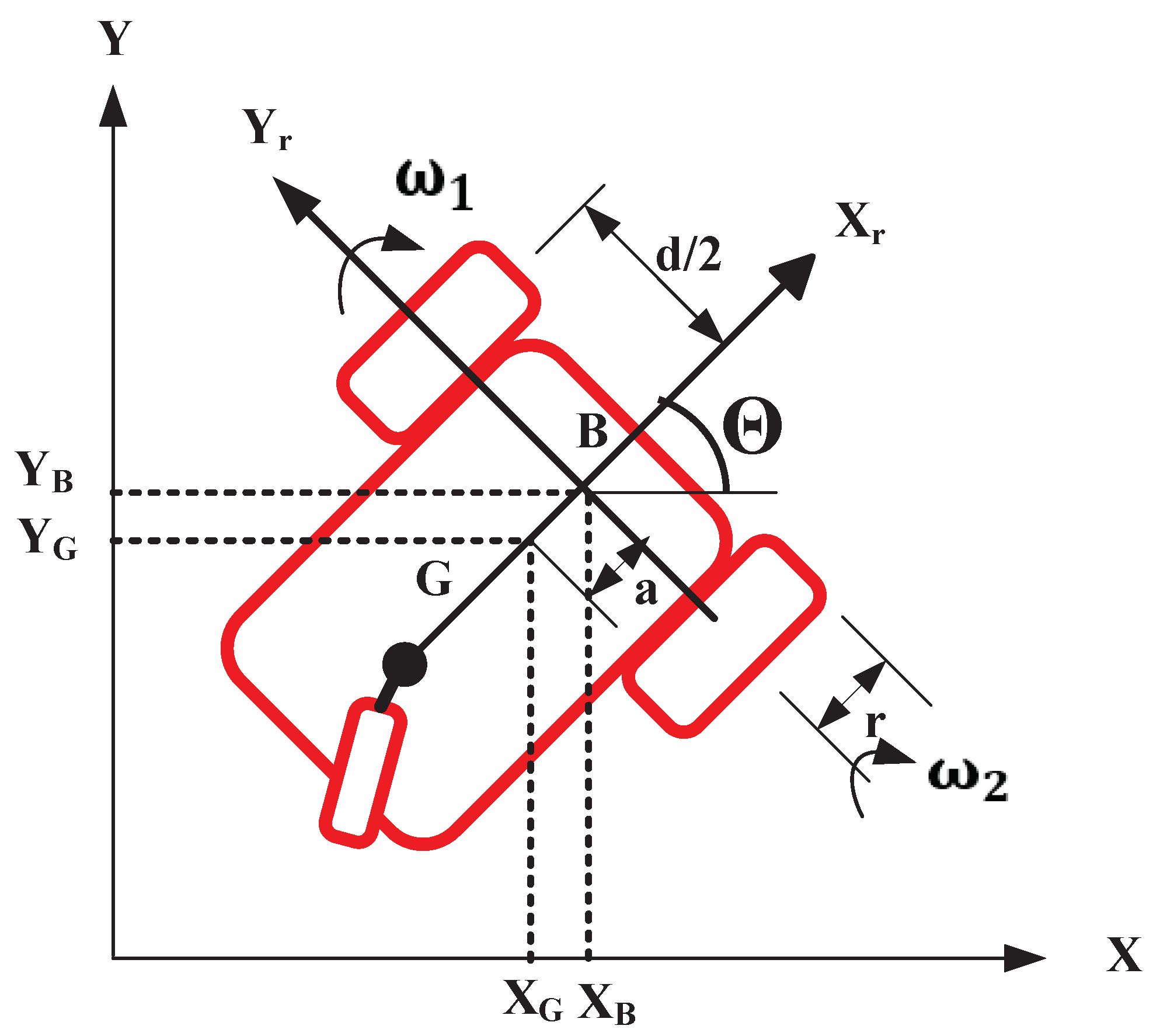
5. System Description for a Mobile Robot

The absolute position of the robot can be represented in the Cartesian plane, with respect to the global frame, by the following three variables as

$$p={\left[x,y,\theta \right]}^T,$$

(36)

where x and y denote the coordinates of the robot center of the mass, while $\theta$ represents the robot orientation, as illustrated in Figure 3. The robot can be controlled by

$$q={\left[\upsilon ,w\right]}^T,$$

(37)

where $\left[\upsilon ,w\right]$ are the linear and angular velocities, respectively. Therefore, the mobile robot kinematic model can be described by the following equation:

$$\left[\begin{array}{c}\dot{x}\\ \dot{y}\\ \dot{\theta }\end{array}\right]=\left[\begin{array}{cc}cos\theta & 0\\ -sin\theta & 0\\ 0& 1\end{array}\right]\left[\begin{array}{c}\upsilon \\ w\end{array}\right].$$

(38)

Our mobile robot belongs to the class of differential-drive ground robots. Hence, the linear and angular velocities can be described using the left $V_l$ and right $V_r$ wheels as follows [4,45]:

$$\begin{array}{ccc}\upsilon & =& \frac{V_l+V_r}{2},\end{array}$$

(39)

$$\begin{array}{ccc}w& =& \frac{V_r-V_l}{d},\end{array}$$

(40)

where d is the distance between wheels. The robot rotation radius, r, can be computed as

$$\begin{array}{ccc}r& =& \frac{d\left(V_l+V_r\right)}{2\left(V_r-V_l\right)}=\frac{\upsilon }{w}.\end{array}$$

(41)

Lastly, the full kinematic model of a mobile robot can be represented as follows:

$$\left[\begin{array}{c}\dot{x}\\ \dot{y}\\ \dot{\theta }\end{array}\right]=\left[\begin{array}{cc}\frac{r\left(dcos\theta -asin\theta \right)}{2d}& \frac{r\left(dcos\theta +asin\theta \right)}{2d}\\ \frac{r\left(dsin\theta -acos\theta \right)}{2d}& \frac{r\left(dsin\theta -acos\theta \right)}{2d}\\ \frac{r}{2d}& \frac{-r}{2d}\end{array}\right]\left[\begin{array}{c}{w}_r\\ w_l\end{array}\right],$$

(42)

where $\left[w_r,w_l\right]$ are the right- and left-wheel angular speeds, respectively. The dynamic model of the mobile robot can be represented using the Euler–Lagrangian method in the following form [46]:

$$M\left(q\right)\left(\ddot{q}\right)+C(q,\dot{q})\left(\dot{q}\right)+F\left(\dot{q}\right)=B\left(q\right)u-A\left(Q\right)\nabla ,$$

(43)

where $M\left(q\right)$ is the inertia matrix; $\dot{q}$ represents the velocity vector of both position and orientation; $\ddot{q}$ denotes the acceleration vector of position and direction; $C(q,\dot{q})$ denotes the Centripetal/Coriolis matrix; $F\left(\dot{q}\right)$ represents a friction vector; $A\left(q\right)$ is a constraint matrix; $B\left(q\right)$ is the input transformation matrix; u is the control input vector; and ∇ denotes a Lagrange multiplier vector.

6. Results and Discussion

In the following section, the effectiveness of the proposed control system is investigated under three different scenarios. First, the proposed method is utilized to regulate the dynamics of a differential-drive mobile robot to follow the desired trajectory in nominal conditions. Second, band-limited white noise was injected into the feedback loop using a MATLAB/SIMULINK block. Third, an external disturbance was added to the system’s dynamics as $d_x=2cos\left(t\right)$ for the x-axis and $d_y=2sin\left(t\right)$ for the y-axis. T2-EFCS initial parameters are given as follows: ${\widehat{\overline{m}}}_{mn}=0.8$, ${\widehat{\underline{m}}}_{mn}=0.5$, ${\widehat{\sigma }}_{mn}=0.55$, ${\widehat{W}}_{nk}=0$, ${\widehat{\eta }}_m=0.5$, ${\widehat{\eta }}_{\sigma }=0.01$, and ${\widehat{\eta }}_W=0.3$. In addition, the efficacy of the proposed method is compared with three other controllers, namely, type-1 fuzzy logic control (T1-FLC), type-2 fuzzy logic control (T2-FLC), and a type-1 evolving fuzzy control system (T1-EFCS). The root mean square error (RMSE) criterion is utilized to evaluate the performance of the proposed control system. The prior threshold values are chosen as $T_{add}=0.11$ and $T_{del}=0.07$. The desired/reference trajectory of the mobile robot can be represented as $p_r={[x_r,y_r,{\theta }_r]}^T$, where we use the velocity reference model to obtain the expected velocity as $q_r\left(t\right)=[v_r,w_r]$. Therefore, the velocity error can be defined by

$$e_{desired}=q_r-q={[e_v,e_w]}^T.$$

(44)

In the simulation model, the following parameters are set as: $m=10$ kg; $r=0.05$ m; $d=0.4$ m; and $F\left(\dot{q}\right)=0$. The desired trajectory is set to follow a sine wave reference for the x-axis, and a cosine wave reference for the y-axis.

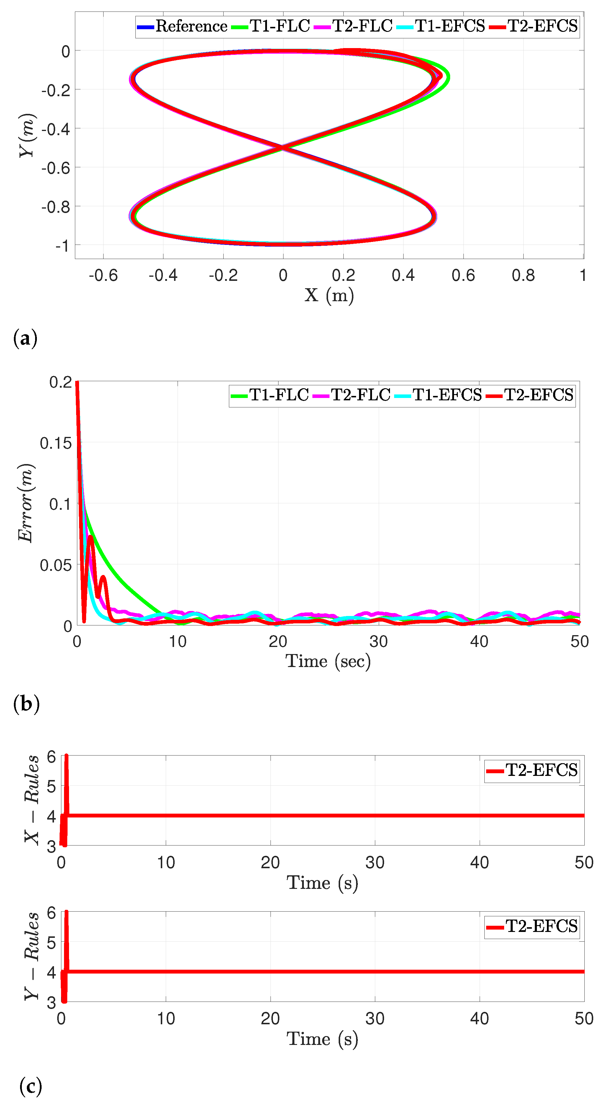
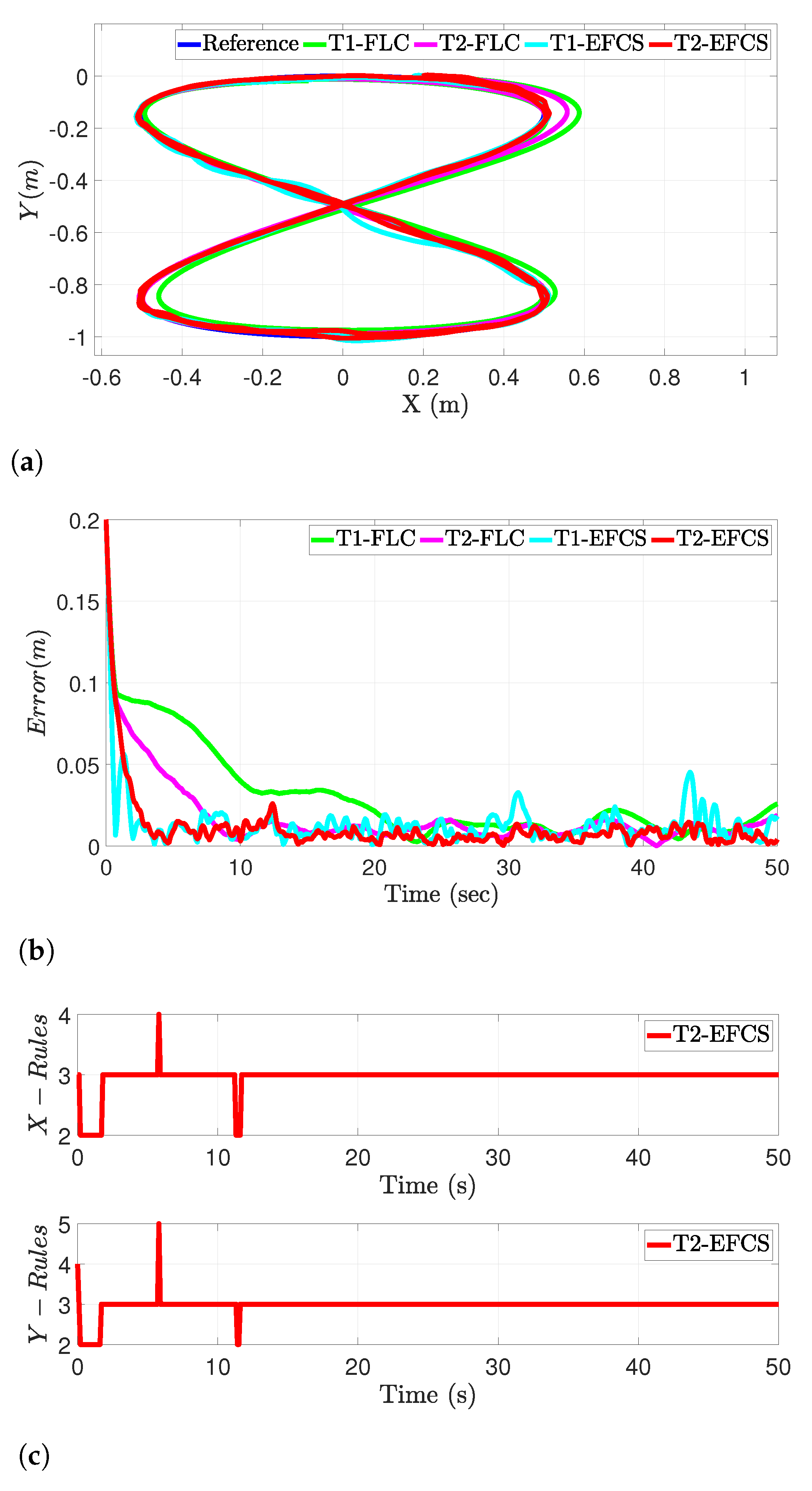
6.1. Performance in Nominal Condition

As depicted in Figure 4a, the simulation results for different controllers for position control in the $xy$-axes are presented, where the proposed T2-EFCS achieved a favorable tracking performance compared to other benchmark controllers demonstrated by their RMSE values in

Table 1. Summary of the experimental comparison of the performance of different controllers.

RMSE Values (Nominal Condition)
Metrics	${\mathit{Error}}_{\mathit{x}}\left[\mathit{m}\right]$	${\mathit{Error}}_{\mathit{y}}\left[\mathbf{m}\right]$	${\mathit{Error}}_{\mathit{dis}}\left[\mathit{m}\right]$
T1−FLC	0.025	0.006	0.026
T2−FLC	0.021	0.005	0.022
T1−EFCS	0.018	0.004	0.019
T2−EFCS	0.017	0.005	0.018

. Moreover, the distance error between the desired and the actual trajectory for the four controllers is illustrated in Figure 4b, where the error decreased from around $0.19$ m to almost zero value in a very short time using our proposed method. Since the proposed T2-EFCS evolves with time, it is important to report the evolving rules with respect to the simulation time. It can be seen in Figure 4c that few rules were required to track the desired trajectory using T2-EFCS. This clearly indicates the simplicity of the proposed control algorithm, making it suitable for small systems with limited computational payloads.

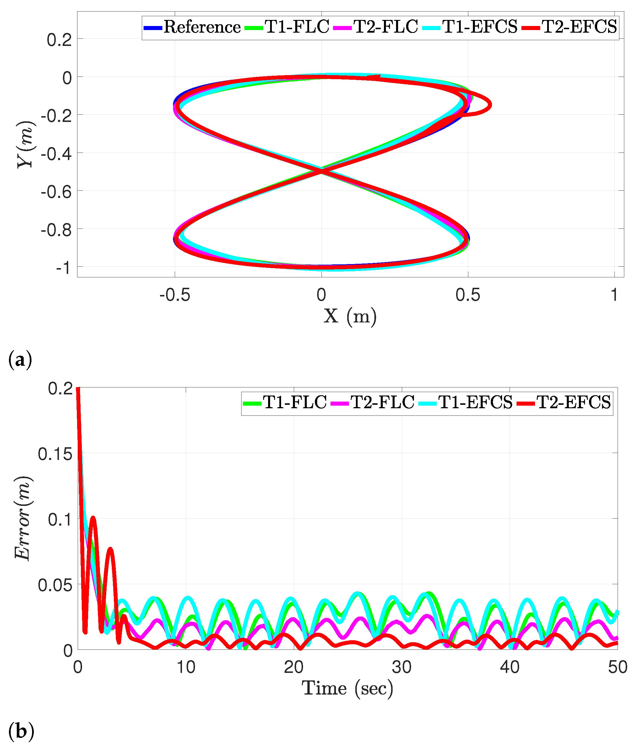
6.2. Performance in the Face of Measurement Noise

In this section, the robustness analysis is presented by injecting a band-limited white noise into the feedback loop using a MATLAB/SIMULINK block. The position tracking in the $xy$-axes is shown in Figure 5a. The simulation results illustrate that the proposed evolving method can handle the disturbance within a reasonable period of time. Additionally, the distance error between the desired and the actual trajectory for the four controllers is plotted in Figure 5b. Lower RMSE values were obtained using the proposed method compared to other benchmark control systems as tabulated in

Table 2. Summary of the experimental comparison of the performance of different controllers in the face of measurement noise.

RMSE Values (Uncertain Condition-Noisy Sensor Data)
Metrics	${\mathit{Error}}_{\mathit{x}}\left[\mathit{m}\right]$	${\mathit{Error}}_{\mathit{y}}\left[\mathit{m}\right]$	${\mathit{Error}}_{\mathit{dis}}\left[\mathit{m}\right]$
T1−FLC	0.0391	0.012	0.041
T2−FLC	0.0269	0.008	0.028
T1−EFCS	0.019	0.010	0.021
T2−EFCS	0.020	0.006	0.021

. Lastly, the fuzzy rules were pruned according to the plant’s dynamics to accommodate measurement noise as shown in Figure 5c.

6.3. Performance under Unknown Disturbance

Additionally, the controller’s performance was assessed by observing the tracking performance in the face of external disturbance. The position tracking in the $xy$-axes under external disturbance is shown in Figure 6a, where the simulation results illustrated the efficacy of the proposed method to handle the external disturbances. Similarly, the RMSE criterion was used for comparing the tracking performance with benchmark controllers as presented in

Table 3. Summary of the experimental comparison of the performance of different controllers in the face of external disturbance.

RMSE Values (Uncertain Condition-External Disturbance)
Metrics	${\mathit{Error}}_{\mathit{x}}\left[\mathit{m}\right]$	${\mathit{Error}}_{\mathit{y}}\left[\mathit{m}\right]$	${\mathit{Error}}_{\mathit{dis}}\left[\mathit{m}\right]$
T1−FLC	0.0307	0.0140	0.0337
T2−FLC	0.0232	0.0112	0.0258
T1−EFCS	0.0306	0.0164	0.0347
T2−EFCS	0.0224	0.0049	0.0229

. The distance error between the desired and the actual trajectory for the four controllers is plotted in Figure 6b. Lastly, more fuzzy rules evolved to face uncertainties as shown in Figure 6c.

7. Conclusions

This paper proposed a novel type-2 evolving fuzzy controller, named the T2-EFLCS, for uncertain dynamic systems. The proposed method was implemented to regulate the dynamics of a mobile robot system. The proposed technique has the ability to perform self-learning and prune its fuzzy rules efficiently. Our approach is useful for reducing the computational complexity and memory requirements of the system, and improving its interpretability and generalization ability, which leads to an optimized fuzzy control system.

To investigate the robustness of T2-EFLCS, an external disturbance was added to the nonlinear model, where simulation results depicted that T2-EFLCS can handle uncertainties in the system. Moreover, lower RMSE values were reported from the proposed T2-EFLCS compared to other controllers. The integration of self-evolving approaches with the SMC-based adaptive law resulted in a fast learning and compact structure. The proposed T2-EFCS was computationally efficient while maintaining superior control performance. The newly developed method leverages the advantages of evolving fuzzy systems for controlling uncertain nonlinear systems.

For future work, this approach can be extended by applying it to a physical robotic system to validate the theoretical results obtained from simulation and to provide insights into practical implementation issues.

References

1. Chwa, D. Fuzzy adaptive tracking control of wheeled mobile robots with state-dependent kinematic and dynamic disturbances. IEEE Trans. Fuzzy Syst. 2011, 20, 587–593. [Google Scholar] [CrossRef]
2. Al-Mayyahi, A.; Wang, W.; Birch, P. Adaptive Neuro-Fuzzy Technique for Autonomous Ground Vehicle Navigation. Robotics 2014, 3, 349–370. [Google Scholar] [CrossRef] [Green Version]
3. Baturone, I.; Moreno-Velo, F.J.; Blanco, V.; Ferruz, J. Design of embedded DSP-based fuzzy controllers for autonomous mobile robots. IEEE Trans. Ind. Electron. 2008, 55, 928–936. [Google Scholar] [CrossRef] [Green Version]
4. Kim, C.J.; Chwa, D. Obstacle Avoidance Method for Wheeled Mobile Robots Using Interval Type-2 Fuzzy Neural Network. IEEE Trans. Fuzzy Syst. 2015, 23, 677–687. [Google Scholar] [CrossRef]
5. Chwa, D. Tracking control of differential-drive wheeled mobile robots using a backstepping-like feedback linearization. IEEE Trans. Syst. Man Cybern. Part A Syst. Hum. 2010, 40, 1285–1295. [Google Scholar] [CrossRef]
6. Zou, J.; Schueller, J.K. Adaptive backstepping control for parallel robot with uncertainties in dynamics and kinematics. Robotica 2014, 32, 2. [Google Scholar] [CrossRef]
7. Lu, X.; Zhao, Y.; Liu, M. Self-learning interval type-2 fuzzy neural network controllers for trajectory control of a Delta parallel robot. Neurocomputing 2018, 283, 107–119. [Google Scholar] [CrossRef]
8. Al-Mahturi, A.; Santoso, F.; Garratt, M.A.; Anavatti, S.G. A Robust Adaptive Interval Type-2 Fuzzy Control for Autonomous Underwater Vehicles. In Proceedings of the 2019 IEEE International Conference on Industry 4.0, Artificial Intelligence, and Communications Technology (IAICT), Bali, Indonesia, 1–3 July 2019; pp. 19–24. [Google Scholar] [CrossRef]
9. Al-Mahturi, A. Development of Self-Learning Type-2 Fuzzy Systems for System Identification and Control of Autonomous Systems. Ph.D. Thesis, UNSW Canberra, Canberra, Australia, 2021. [Google Scholar] [CrossRef]
10. Juang, C.F.; Chang, Y.C. Evolutionary-group-based particle-swarm-optimized fuzzy controller with application to mobile-robot navigation in unknown environments. IEEE Trans. Fuzzy Syst. 2011, 19, 379–392. [Google Scholar] [CrossRef]
11. Al-Mahturi, A.; Santoso, F.; Garratt, M.A.; Anavatti, S.G. A Robust Self-Adaptive Interval Type-2 TS Fuzzy Logic for Controlling Multi-Input–Multi-Output Nonlinear Uncertain Dynamical Systems. IEEE Trans. Syst. Man Cybern. Syst. 2022, 52, 655–666. [Google Scholar] [CrossRef]
12. Al-Mahturi, A.; Santoso, F.; Garratt, M.A.; Anavatti, S.G. Online System Identification for Nonlinear Uncertain Dynamical Systems Using Recursive Interval Type-2 TS Fuzzy C-means Clustering. In Proceedings of the 2020 IEEE Symposium Series on Computational Intelligence (SSCI), Canberra, Australia, 1–4 December 2020; pp. 1695–1701. [Google Scholar] [CrossRef]
13. Huang, J.; Ri, M.; Wu, D.; Ri, S. Interval Type-2 fuzzy logic modeling and control of a mobile two-wheeled inverted pendulum. IEEE Trans. Fuzzy Syst. 2017, 26, 2030–2038. [Google Scholar] [CrossRef]
14. Al-Mahturi, A.; Santoso, F.; Garratt, M.A.; Anavatti, S.G. Self-Learning in Aerial Robotics Using Type-2 Fuzzy Systems: Case Study in Hovering Quadrotor Flight Control. IEEE Access 2021, 9, 119520–119532. [Google Scholar] [CrossRef]
15. Al-Mahturi, A.; Santoso, F.; Garratt, M.A.; Anavatti, S.G. An Intelligent Control of an Inverted Pendulum Based on an Adaptive Interval Type-2 Fuzzy Inference System. In Proceedings of the 2019 IEEE International Conference on Fuzzy Systems (FUZZ-IEEE), New Orleans, LA, USA, 23–26 June 2019; pp. 1–6. [Google Scholar] [CrossRef]
16. Shi, Y.; Eberhart, R.; Chen, Y. Implementation of evolutionary fuzzy systems. IEEE Trans. Fuzzy Syst. 1999, 7, 109–119. [Google Scholar] [CrossRef] [Green Version]
17. Kasabov, N.K. Evolving Connectionist Systems: The Knowledge Engineering Approach; Springer Science & Business Media: Berlin/Heidelberg, Germany, 2007. [Google Scholar]
18. Škrjanc, I.; Iglesias, J.A.; Sanchis, A.; Leite, D.; Lughofer, E.; Gomide, F. Evolving fuzzy and neuro-fuzzy approaches in clustering, regression, identification, and classification: A survey. Inf. Sci. 2019, 490, 344–368. [Google Scholar] [CrossRef]
19. Angelov, P.P. Evolving Rule-Based Models: A Tool for Design of Flexible Adaptive Systems; Physica; Springer: Berlin/Heidelberg, Germany, 2013; Volume 92. [Google Scholar]
20. Lughofer, E.; Pratama, M. Online active learning in data stream regression using uncertainty sampling based on evolving generalized fuzzy models. IEEE Trans. Fuzzy Syst. 2017, 26, 292–309. [Google Scholar] [CrossRef]
21. Al-Mahturi, A.; Santoso, F.; Garratt, M.A.; Anavatti, S.G. A Simplified Model-Free Self-Evolving TS Fuzzy Controller for Nonlinear Systems with Uncertainties. In Proceedings of the 2020 IEEE Conference on Evolving and Adaptive Intelligent Systems (EAIS), Bari, Italy, 27–29 May 2020; pp. 1–6. [Google Scholar] [CrossRef]
22. Juang, C.F.; Lin, C.T. An online self-constructing neural fuzzy inference network and its applications. IEEE Trans. Fuzzy Syst. 1998, 6, 12–32. [Google Scholar] [CrossRef]
23. Kasabov, N.K.; Song, Q. DENFIS: Dynamic evolving neural-fuzzy inference system and its application for time-series prediction. IEEE Trans. Fuzzy Syst. 2002, 10, 144–154. [Google Scholar] [CrossRef] [Green Version]
24. Angelov, P.; Filev, D. Simpl_eTS: A simplified method for learning evolving Takagi-Sugeno fuzzy models. In Proceedings of the The 14th IEEE International Conference on Fuzzy Systems, Changsha, China, 27–29 August 2005; pp. 1068–1073. [Google Scholar] [CrossRef] [Green Version]
25. Rong, H.J.; Sundararajan, N.; Huang, G.B.; Saratchandran, P. Sequential Adaptive Fuzzy Inference System (SAFIS) for nonlinear system identification and prediction. Fuzzy Sets Syst. 2006, 157, 1260–1275. [Google Scholar] [CrossRef]
26. Angelov, P. Evolving Takagi-Sugeno fuzzy systems from streaming data (eTS+). In Evolving Intelligent Systems: Methodology and Applications; Wiley Online Library: Hoboken, NJ, USA, 2010; Volume 12, p. 21. [Google Scholar]
27. Pratama, M.; Anavatti, S.G.; Angelov, P.P.; Lughofer, E. PANFIS: A Novel Incremental Learning Machine. IEEE Trans. Neural Netw. Learn. Syst. 2014, 25, 55–68. [Google Scholar] [CrossRef]
28. Ferdaus, M.M.; Pratama, M.; Anavatti, S.; Garratt, M.A.; Pan, Y. Generic evolving self-organizing neuro-fuzzy control of bio-inspired unmanned aerial vehicles. IEEE Trans. Fuzzy Syst. 2019. [Google Scholar] [CrossRef] [Green Version]
29. Hsu, C.F.; Wong, K.Y. On-line constructive fuzzy sliding-mode control for voice coil motors. Appl. Soft Comput. 2016, 47, 415–423. [Google Scholar] [CrossRef]
30. Rong, H.J.; Yang, Z.X.; Wong, P.K.; Vong, C.M.; Zhao, G.S. Self-evolving fuzzy model-based controller with online structure and parameter learning for hypersonic vehicle. Aerosp. Sci. Technol. 2017, 64, 1–15. [Google Scholar] [CrossRef]
31. Juang, C.F.; Lu, C.F.; Tsao, Y.W. A Self-Evolving Interval Type-2 Fuzzy Neural Network for Nonlinear Systems Identification. IFAC Proc. Vol. 2008, 41, 7588–7593. [Google Scholar] [CrossRef] [Green Version]
32. Juang, C.F.; Tsao, Y.W. A Type-2 Self-Organizing Neural Fuzzy System and Its FPGA Implementation. IEEE Trans. Syst. Man Cybern. Part B Cybern. 2008, 38, 1537–1548. [Google Scholar] [CrossRef]
33. Hassanein, O.; Anavatti, S.G.; Shim, H.; Salman, S.A. Auto-generating fuzzy system modelling of physical systems. In Proceedings of the 2015 IEEE Conference on Control Applications (CCA), Sydney, Australia, 21–23 September 2015; pp. 1142–1147. [Google Scholar]
34. Chen, C.H.; Lin, C.J.; Lin, C.T. A functional-link-based neurofuzzy network for nonlinear system control. IEEE Trans. Fuzzy Syst. 2008, 16, 1362–1378. [Google Scholar] [CrossRef]
35. Pratama, M.; Lu, J.; Zhang, G. Evolving type-2 fuzzy classifier. IEEE Trans. Fuzzy Syst. 2016, 24, 574–589. [Google Scholar] [CrossRef]
36. Lin, C.M.; Le, T.L.; Huynh, T.T. Self-evolving function-link interval Type-2 fuzzy neural network for nonlinear system identification and control. Neurocomputing 2018, 275, 2239–2250. [Google Scholar] [CrossRef]
37. Chen, C.S.; Lin, W.C. Self-adaptive interval Type-2 neural fuzzy network control for PMLSM drives. Expert Syst. Appl. 2011, 38, 14679–14689. [Google Scholar] [CrossRef]
38. Le, T.L.; Lin, C.M.; Huynh, T.T. Self-evolving type-2 fuzzy brain emotional learning control design for chaotic systems using PSO. Appl. Soft Comput. 2018, 73, 418–433. [Google Scholar] [CrossRef]
39. Lin, C.M.; Chen, T.Y. Self-organizing CMAC control for a class of MIMO uncertain nonlinear systems. IEEE Trans. Neural Netw. 2009, 20, 1377–1384. [Google Scholar] [CrossRef] [PubMed]
40. Le, T.L.; Huynh, T.T.; Lin, C.M. Self-Evolving Interval Type-2 Wavelet Cerebellar Model Articulation Control Design for Uncertain Nonlinear Systems Using PSO. Int. J. Fuzzy Syst. 2019, 21, 2524–2541. [Google Scholar] [CrossRef]
41. Al-Mahturi, A.; Santoso, F.; Garratt, M.A.; Anavatti, S.G. Modeling and Control of a Quadrotor Unmanned Aerial Vehicle Using Type-2 Fuzzy Systems. In Unmanned Aerial Systems: Theoretical Foundation and Applications; Elsevier: Amsterdam, The Netherlands, 2020. [Google Scholar]
42. Lin, Y.Y.; Liao, S.H.; Chang, J.Y.; Lin, C.T. Simplified interval type-2 fuzzy neural networks. IEEE Trans. Neural Netw. Learning Syst. 2014, 25, 959–969. [Google Scholar] [CrossRef] [PubMed]
43. Al-Mahasneh, A.J.; Anavatti, S.; Garratt, M. Self-Evolving Neural Control for a Class of Nonlinear Discrete-Time Dynamic Systems with Unknown Dynamics and Unknown Disturbances. IEEE Trans. Ind. Inform. 2019, 16, 6518–6529. [Google Scholar] [CrossRef]
44. Saghafinia, A.; Ping, H.W.; Uddin, M.N.; Gaeid, K.S. Adaptive fuzzy sliding-mode control into chattering-free IM drive. IEEE Trans. Ind. Appl. 2014, 51, 692–701. [Google Scholar] [CrossRef]
45. Martins, F.N.; Celeste, W.C.; Carelli, R.; Sarcinelli-Filho, M.; Bastos-Filho, T.F. An adaptive dynamic controller for autonomous mobile robot trajectory tracking. Control. Eng. Pract. 2008, 16, 1354–1363. [Google Scholar] [CrossRef]
46. Zhang, J.; Li, Q.; Chang, X.; Chao, F.; Lin, C.M.; Yang, L.; Huynh, T.T.; Zheng, L.; Zhou, C.; Shang, C. A Novel Self-Organizing Emotional CMAC Network for Robotic Control. In Proceedings of the 2020 International Joint Conference on Neural Networks (IJCNN), Glasgow, UK, 19–24 July 2020; pp. 1–6. [Google Scholar]
Figure 1. Interval type-2 Gaussian membership function.
Robotics 12 00040 g001
Figure 2. Flowchart of our proposed T2-EFCS.
Robotics 12 00040 g002
Figure 3. Kinematic model of the differential-drive mobile robot.
Robotics 12 00040 g003
Figure 4. Performance of the proposed control system in nominal condition. (a) Desired vs. actual positions of the robot path in nominal condition. (b) Distance error evolution for different controllers. (c) Evolution of the fuzzy rules for the proposed T2-EFCS.
Robotics 12 00040 g004
Figure 5. Performance of the proposed system in the face of measurement noise. (a) Desired vs. actual positions of the robot path in the face of sensor noise. (b) Distance error evolution for different controllers in the face of measurement noise. (c) Evolution of the fuzzy rules for T2-EFCS in the face of measurement noise.
Robotics 12 00040 g005
Figure 6. Performance of the proposed system in the face of external disturbance. (a) Desired vs. actual positions of the robot path in the face of external disturbance. (b) Distance error evolution for different controllers in the face of external disturbance. (c) Evolution of the fuzzy rules for the proposed T2-EFCS in the face of external disturbance.
Robotics 12 00040 g006aRobotics 12 00040 g006b