Article

Edge AI-Based Tree Trunk Detection for Forestry Monitoring Robotics

by
Daniel Queirós da Silva
1,2,*,†,
Filipe Neves dos Santos
1,
Vítor Filipe
1,2,
Armando Jorge Sousa
1,3 and
Paulo Moura Oliveira
1,2
1
INESC Technology and Science (INESC TEC), 4200-465 Porto, Portugal
2
School of Science and Technology, University of Trás-os-Montes e Alto Douro (UTAD), 5000-801 Vila Real, Portugal
3
Faculty of Engineering, University of Porto (FEUP), 4200-465 Porto, Portugal
*
Author to whom correspondence should be addressed.
Current address: Campus da FEUP, Rua Dr. Roberto Frias 400, 4200-465 Porto, Portugal.
Robotics 2022, 11(6), 136; https://doi.org/10.3390/robotics11060136
Submission received: 2 November 2022 / Revised: 22 November 2022 / Accepted: 24 November 2022 / Published: 27 November 2022
(This article belongs to the Special Issue Robotics and AI for Precision Agriculture)

Abstract

:
Object identification, such as tree trunk detection, is fundamental for forest robotics. Intelligent vision systems are of paramount importance in order to improve robotic perception, thus enhancing the autonomy of forest robots. To that purpose, this paper presents three contributions: an open dataset of 5325 annotated forest images; a tree trunk detection Edge AI benchmark between 13 deep learning models evaluated on four edge-devices (CPU, TPU, GPU and VPU); and a tree trunk mapping experiment using an OAK-D as a sensing device. The results showed that YOLOR was the most reliable trunk detector, achieving a maximum F1 score around 90% while maintaining high scores for different confidence levels; in terms of inference time, YOLOv4 Tiny was the fastest model, attaining 1.93 ms on the GPU. YOLOv7 Tiny presented the best trade-off between detection accuracy and speed, with average inference times under 4 ms on the GPU considering different input resolutions and at the same time achieving an F1 score similar to YOLOR. This work will enable the development of advanced artificial vision systems for robotics in forestry monitoring operations.

1. Introduction

In recent years, the increasing occurrence of wildfires across Europe (and all over the world) served as a warning that a better management of the forest is needed. An optimised forest management process will enable to reduce the losses during the fires events. Forest represents up to 38% of the total land surface of the European Union countries [1], making this a very relevant societal and ecological issue.
Over the years, the scientific community has been proposing several works aiming at better forest monitoring and care by means of imagery methods. Some are to prevent and detect diseases in forest trees using Deep Learning (DL) and Unmanned Aerial Vehicle (UAV) imagery [2,3,4] or satellite high-resolution imagery [5]. The use of UAVs as a remote sensing platform is also a common way of detecting dead trees individually [6] or in clusters [7], as this can help prevent the occurrence of wildfires. The early detection of wildfires can help prevent their progress over forest lands, hence reducing their ecological and societal impact. Other ways of detecting forest fires are about segmentation of burned areas in UAV images [8], flame detection [9,10,11], flame segmentation [12,13,14,15] or smoke detection [16] with DL in terrestrial and aerial images. These works can enable an early alert to firefighters about the appearance of a possible forest fire, thus increasing forest protection and, consequently, forest monitoring. From UAVs to terrestrial vehicles, the monitoring of the forest areas and forest inventory can be improved with the help of robotics with advanced intelligent perception systems.
The use of robotics in forestry has made slow progress mostly due to some inherent problems that exist in forests: variations of temperature and humidity, steep slope and harsh terrains, and the general complexity of such environment with high probability of appearing wild animals and several obstacles, such as boulders, bushes, holes and fallen trees [17]. Nevertheless, some terrestrial [18,19,20,21] and aerial [22,23,24] robotic platforms have been developed that can contribute to improve forest protection and monitoring. However, there are terrain-independent aspects that can compromise the performance of a robot in a forest such as the absence of good communication means, since Global Navigation Satellite System (GNSS) and internet connection, in general, do not work well enough in this domain [25]. Hence, advanced perception solutions are needed to make robots capable of working under such difficult conditions.
Robotic visual perception in forestry contexts is a topic that has been developing within the scientific community and plays an important role in the way robots perceive the world. Back in 2011, a work about 3D log (a tree trunk that was cut off) recognition and respective pose estimation for log grasping operations was proposed [26]. By means of a structured light camera, the authors were capable of extracting 3D information about the logs and, after some 3D segmentation steps and an extrinsic calibration, they reconstructed the logs and estimated their respective poses. The authors concluded that the reconstruction errors increased exponentially relatively to the distance to the logs, and that best results were obtained under 3 m. Another work where the authors proposed the 3D detection of tree trunks by means of cameras (in this case a stereo-pair) was presented in [27]. Here, a DL-based 3D object detector was trained on point clouds of tree trunks acquired with a ZED Stereo 2 camera. The authors concluded that their 3D recognition system was capable of accurately detecting tree trunks at ranges up to 7 m. Although 3D information about the surroundings is important for robots for mapping and navigation purposes, the go-to way of handling the data provided by cameras is 2D. More recently, some works have been published about tree trunks detection in images (in 2D): some detected tree trunks in street images [28,29], others focused on detecting tree trunks in forest contexts [30], while others detected stumps in harvested forest areas [31]. In [32], instead of only detecting logs, it was aimed at the detection and segmentation of logs for grasping operations. For that, they trained and tested several DL-based object segmentation methods, and they concluded that such perception methods and systems can be used as an assistance tool for operators or even for fully autonomous operations in the forestry domain.
Even though some advances have been made in recent years regarding robotic visual perception, more work needs to be completed in order to attain safer and smarter robotic systems to work in forests semi or fully autonomously. With this in mind, this work produced a study and a use case about forest tree trunks detection and mapping, using Edge Artificial Intelligence (AI), to support monitoring operations in forests. Edge AI approaches are important for robotics in general, since it allows running DL-based models and algorithms on specific hardware devices that can be placed on the robot itself. So, instead of running these models on self-managed servers or using a cloud service (which always account with some additional communication latency), the models can be run locally, hence improving performance, in terms of speed, of the robotics tasks that rely on them.
This work contributes to the knowledge domain with three contributions:
  • Public dataset of forest images fully annotated;
  • Benchmark between four different edge-computing hardware and 13 DL models;
  • Use case of tree trunks mapping using one DL model combined with an AI-enabled vision device.
This article is structured as follows: Section 2 reviews the state-of-the-art of cutting-edge DL models that were used in this work, Section 3 presents the dataset built in this study, shows some details about the edge-devices used to test the object detection models and specifies the training and testing conditions of the DL models. Section 4 presents the obtained testing results in terms of tree trunks detection precision, inference time and the accuracy of tree trunks mapping. Section 5 discusses the obtained results, and Section 6 ends this paper presenting the main conclusions and future work.

2. Deep Learning-Based Object Detection Methods

This section presents the DL models that were used in this work to detect forest tree trunks. The DL methods that were used are the following: Single-Shot Detector (SSD) [33] combined with MobileNet V1 [34], MobileNet V2 [35] and MobileNet V3 (Small and Large) [36], three light versions of EfficientDet [37], a tiny version of YOLOv4 [38], two light versions of YOLOv5 (https://doi.org/10.5281/zenodo.3908559, accessed on 26 July 2022), a tiny version of YOLOv7 [39], a combination of Cross Stage Partial network (CSP) [40] with YOLOR [41], and a Vision Transformer-based detector called DETR [42].
Single Shot Detector (SSD) [33] is an object detector that generates a set of candidate bounding boxes with different scales and aspect ratios. At prediction time, the bounding boxes are scored considering whether an object is present within the box or not. In the affirmative case, the box is adjusted to better fit the object.
MobileNets [34] are very light and efficient neural network models created for embedded and mobile applications. They are formed by depth-wise separable convolutions that make the model smaller and computationally lighter. In addition, two hyper-parameters were implemented which, when tweaked, allow to improve the accuracy and/or speed of the model. The second version of MobileNets (MobileNet V2) [35] appeared in 2019 and brought some improvements regarding inference speed and model’s size comparatively with the previous version. Such improvements were enabled by the implementation of inverted residuals and linear bottlenecks. The third and last version of MobileNets (MobileNet V3) [36] was published in late 2019, and it was designed for mobile phones applications. This was achieved by combining a hardware-aware network architecture search with a method that takes the best found architecture and fine-tunes the same until a certain speed is attained. From this work, two variations of MobileNet V3 appeared: a smaller and a larger one. In general, MobileNet V3 Small is faster and Mobilenet V3 Large is more accurate than MobileNet V1 and V2.
EfficientDets [37] are a family of object detectors that are more efficient and less computationally expensive that prior state-of-the-art detectors. The major improvements made with these detectors are the implementation of a weighted bi-directional feature pyramid network responsible for a fast multi-scale fusion of features, and a method that uniformly scales the depth, width and resolution for all architecture compounds at the same time.
You Only Look Once (YOLO) [43] is a single-stage object detection network that predicts and scores bounding boxes in one run from full images. YOLO divides the input image into a grid of cells, and for each cell, it predicts bounding boxes, their confidences and associated class likelihoods. YOLO proved to be a reliable real-time object detector achieving processing frequencies of 45 Hz and 155 Hz with its base and smaller models, respectively, while gathering competitive accuracy results with less than real-time detectors. The second [44] and third [45] versions of YOLO (YOLOv2 and YOLOv3) suffered some architecture tweaks that brought improvements for the model in terms of accuracy and speed, outperforming state-of-the-art models at that time, such as SSD. The fourth version of YOLO (YOLOv4) [38] was published in 2020, and the major changes were about the use of new features to attempt improve YOLO. Such features include weighted residual connections, cross-stage partial connections, cross-mini-batch normalisation, self-adversarial training and mish activation. At that time, YOLOv4 was the fastest and more accurate real-time object detector, achieving twice the speed of EfficientDet while keeping a comparable accuracy. YOLOv4 also improved YOLOv3’s precision and speed by 10% and 12%, respectively.
Since YOLOv4, three new versions of YOLO series have appeared. YOLOv5 is the fifth version of YOLO and is considered to be “non-official” by the community. The authors claimed that YOLOv5 achieved better detection and speed performance than previous YOLO versions and other detectors, but they did not provide a real comparison, for instance, with YOLOv4. YOLOv6 [46] corresponds to the YOLO version and was designed to be mainly applied to industrial applications. The more recent new version of YOLO is YOLOv7 [39]. This seventh version is currently the best object detector, surpassing all known state-of-the-art detectors with the highest average precision of 56.8% on the MS COCO dataset [47] and with inference times ranging from 6 up to 200 ms. The authors of [39] contributed to this model with a bag-of-freebies approach to tackle two issues that appeared along the way: replacement of the re-parameterised module and the allocation of dynamic label assignment.
You Only Learn One Representation (YOLOR) [41] is a network that is inspired in the way human experience is learned. In fact, in [41], the authors presented a detector that can encode implicit knowledge (the model learns subconsciously) and explicit knowledge (the model learns from input data), similarly to the human brain that can learn in an explicit (from experience) and implicit way.
DEtection TRansformer (DETR) [42] is an object detector that is based on a Vision Transformer (ViT) [48]. Transformers were recently introduced to tackle Computer Vision (CV) tasks, as they were the standard architecture for natural language processing tasks. ViTs (the transformers applied in vision) attained also great results recognising images compared to the standard Convolutional Neural Networks (CNN) [48] and at the same time needing fewer resources during training. DETR is also based on the transformer architecture, but its main goal is to detect objects in images rather than classify the images. DETR showed comparable results with other detectors, especially with large objects; regarding small objects, the authors claim that it is a challenge to train, optimise and detect these objects.

3. Materials and Methods

This section details the image acquisition process (cameras and platforms that were used to acquire the data), presents the post-processing that was made on the images (data labelling, augmentation operations and pre-train dataset splitting), shows the training environment, model configurations and conversions, and presents the trunk detection evaluation metrics used and the experiments that were performed in this work.

3.1. Image Acquisition Process

The dataset used in this work corresponds to a new version of the dataset presented in [49], with more than 2000 new images and annotations. The images that were added were from a Robot Operating System (ROS) bag dataset presented in [50]. The image dataset was acquired in three different regions of Portugal: Lobão (41°11′22.09″ N, 8°29′55.54″ W), Vila do Conde (41°21′14.22″ N, 8°44′30.66″ W) and Valongo (40°59′05.10″ N, 8°29′17.41″ W). In these regions, eucalyptus and pinus are the predominant tree species. In each forestry area, video footage was captured using five different cameras: FLIR M232 (https://www.flir.eu/products/m232, accessed on 26 July 2022), ZED Stereo (https://www.stereolabs.com/zed, accessed on 26 July 2022), Allied Mako G-125 (https://www.alliedvision.com/en/camera-selector/detail/mako/G-125, accessed on 26 July 2022), OAK-D (https://store.opencv.ai/products/oak-d, accessed on 26 July 2022), and GoPro Hero6 (https://gopro.com/en/gb/update/hero6, accessed on 26 July 2022). Only GoPro was transported by hand during image recording process; the other cameras were mounted on ground robotic vehicles. OAK-D was the only camera that was placed facing sideways; the others were placed pointing towards the front.
The images were extracted from the videos using a sub-sampling methodology and were filtered according to the presence of any defects on them, such as blur or incandescence caused by the sun. The result was a total of 5325 images belonging to different cameras and spectra (visible and thermal images). Table 1 presents some features of the images that are part of the original dataset. Compared to the previous version, this dataset has 2430 more images which were all recorded in Valongo with three of the five cameras: ZED (640 images), FLIR (940 thermal images), and OAK-D (850 images). This new dataset was made publicly available (https://doi.org/10.5281/zenodo.7186052, accessed on 11 October 2022).

3.2. Data Labelling, Augmentation and Splitting

After acquiring images from the forestry areas, those images were labelled using Computer Vision Annotation Tool (CVAT) (https://github.com/opencv/cvat, accessed on 26 July 2022) with the Pascal Visual Object Classes format [51]. All images and their labels from the original dataset went through nine augmentation processes, resulting in each original image being transformed into nine new versions—the nine augmentation operations are explained in Table 2. Dataset augmentation is an important step and must be taken because training DL models require large amounts of data in order to achieve a good performance in unseen data; missing this step could compromise the accuracy of the models. In the end of the augmentation processes, the size of the augmented dataset was about 53,250 images ( 9 × 5325 + 5325 ). However, images without any label (absence of trunks) were discarded. So, the final size of the augmented dataset was actually 49,608 images (3642 images were removed).
Before using the augmented dataset for DL training, the same was split into three subsets: training, validation and testing. The ratios that were used to perform this division were 70% for training, 10% for validation and 20% for testing, so 34,723 images, 4964 images and 9910 images for the train, validation and test sets, respectively. From the test set, two different subsets were considered for testing the DL models: one is made by augmented images and corresponds to 100% of the test set, the other is made by only original (non-augmented) images which comprises 10% of the test set.

3.3. Configuration, Training and Conversion of Deep Learning-Based Object Detection Models

The DL models that were chosen for the task at hand were: SSD MobileNet V1, SSD MobileNet V2, SSD MobileNet V3 Small, SSD MobileNet V3 Large, EfficientDet Lite0, EfficientDet Lite1, EfficientDet Lite2, YOLOv4 Tiny, YOLOv5 Nano, YOLOv5 Small, YOLOv7 Tiny, YOLOR-CSP and DETR-ResNet50. In terms of network architecture, YOLOv4 Tiny was the only model that suffered a minor change, regarding its activation function that originally was Leaky Rectified Linear Unit (ReLU), and we changed it to ReLU.
The SSD-based models were trained using TensorFlow Object Detection Application Programming Interface (API) 1 (https://github.com/tensorflow/models/tree/master/research/object_detection, accessed on 26 July 2022), the three versions of EfficientDet Lite were trained using TensorFlow 2 Lite Model Maker (https://www.tensorflow.org/lite/models/modify/model_maker, accessed on 26 July 2022), YOLOv4 Tiny was trained using Darknet (https://github.com/AlexeyAB/darknet, accessed on 26 July 2022), and the remaining models were trained using PyTorch (https://pytorch.org/, accessed on 26 July 2022).
All models were trained using an NVIDIA GeForce 3090 Graphics Processing Unit (GPU) with 32 GygaByte (GB) of available memory and a compute capability of 35 × 10 12 floating point Operations Per Second (OPS). A transfer learning approach was taken to train the DL models, and their training parameters are defined in Table 3. The learning rate and input resolution were kept default, the batch size was selected according to the GPU memory and the training epochs were chosen in a way that all models’ training loss curves converged with a variation of less than 5%. A relevant aspect to be mentioned is that the input resolution of DETR-ResNet50 can vary between 800 and 1333 pixels in width and height [42]. So, the resolution (indicated with “*” in Table 3) is in fact the maximum input resolution the model can have during training.
After training, 10 models were quantised (weights of 8-bit integer) with success and were converted to run on Coral USB Accelerator’s Tensor Processing Unit (TPU) (https://coral.ai/products/accelerator, accessed on 26 July 2022): SSD-based models were quantised using Quantisation-Aware Training, and EfficientDet Lite models, YOLOv4 Tiny and YOLOv5 models were quantised using Post-Training Quantisation. In order for a model to be fully supported on the TPU, its operations must be supported by the TPU; otherwise, such operations will be run on the Central Processing Unit (CPU) instead on the TPU. So, Table 4 shows the number of supported and unsupported operations and the respective ratio in percentage. It is important to mention that we had to reduce the input resolution of YOLOv5 models to a maximum of 448 × 448 pixels to enable their successful conversion for the TPU.

3.4. Tree Trunks Detection Evaluation, Tree Trunks Mapping and Research Experiments

In this section, the evaluation metrics and edge-devices that were used to perform tree trunks detection are presented. Additionally, the tree trunk mapping algorithm and the research experiments that were conducted in this work are detailed.

3.4.1. Evaluation Metrics and Devices

The models evaluation was made by running inference on the test subset (defined in Section 3.2). Then, the detections outputted from the models were filtered using Non-Maximum Suppression (NMS) with 10% and 60% confidence thresholds and the overlapping threshold, respectively. This way, only detections with confidence above 10% were considered. The metric that was chosen to evaluate accuracy-wise the models was the F1 score, as this metric allows to maximise, at the same time, two well-known metrics in this domain: Precision (measures the detections that are objects) and Recall (measures the objects that are detected).
In addition to evaluating the models in terms of detection accuracy, they were also evaluated in terms of inference time in four different edge-devices, which are presented in Table 5. The NVIDIA GeForce RTX 3090 GPU served as the baseline for the other devices, and the Intel Movidius Myriad X Visual Processing Unit (VPU) of OAK-D was used to deploy some models to perform real-time tree trunks mapping. The lower the inference time of the models, the more likely the models are to perform tasks in real-time.

3.4.2. Tree Trunk Mapping Algorithm

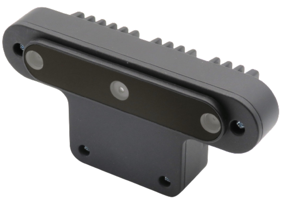
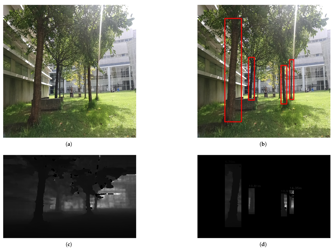
The tree trunk mapping algorithm receives data from an OAK-D perception device, which is shown in Figure 1. This sensing device has an embedded inertial measurement device, one colour camera (at the body centre) and two monochromatic cameras that form a stereo-vision pair for depth processing. Additionally, the OAK-D has a VPU responsible for running the object detection neural network to detect the tree trunks.
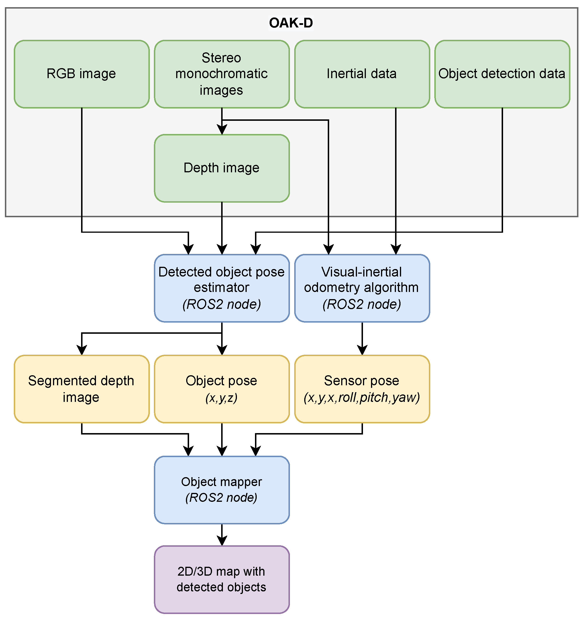
The tree trunk algorithm is summarised by Figure 2. The algorithm starts by receiving the detections made with the centred colour camera which are aligned with the depth images. This way, it is possible to know almost exactly (because depth computation by means of stereo vision has inherent errors) the distance to the detected objects. With such detections, we masked the bounding boxes on the respective depth images, and through a depth thresholding step on the centre point of each bounding box, the objects are segmented. The trunk mapping is made by means of a visual–inertial odometry method (OpenVINS [52]) that uses the stereo images and the inertial data of OAK-D to give an estimation of the six Degrees of Freedom (DoF) relative pose of the device. The final result is a 2D/3D map with the detected tree trunks. An important aspect to be highlighted is that all raw data are processed and made available only by OAK-D.

3.4.3. Tree Trunk Detection Experiments

The experiments conducted in this work were:
  • Original test subset vs. augmented test subset;
  • Non-quantised vs. quantised weights;
  • Decrease of input resolutions for YOLOv5, YOLOv7, YOLOR and DETR models;
  • Evolution of F1 score across several confidence levels;
  • Inference speed in four edge-devices;
  • Tree trunks mapping with an OAK-D.
Experiment #1 is about assessing the detection accuracy of the models, using the F1 score, in the original test data subset versus in the augmented test data subset. Normally, augmentation processes are only applied to the training and/or validation datasets [53], so we have also used augmented images in the test subset to measure the impact of their utilisation for testing DL models.
Experiment #2 is about evaluating the detection accuracy of the quantised models, using the F1 score, compared to their non-quantised variants. Normally, the non-quantised variants of the models are more precise than the quantised ones for the same task, since the weights of the former are in floating point format and, after being quantised, are turned into a less precise floating point format (for instance, from 32-bit floating point precision to 16-bit) or event into an integer format [54].
Experiment #3 is about decreasing the input resolution of higher resolution models, such as YOLOv5, YOLOv7, YOLOR and DETR, in order to observe the variation of detection accuracy and also to make a fair comparison among all models, since the other models have much lower input resolutions than the four aforementioned. The input resolutions selected were 320 × 320 and 448 × 448. The first one was chosen because it was very close to the input resolution of the SSD models and EfficientDet Lite0, the second was chosen because it was close to the remaining EfficientDet Lite’s and YOLOv4’s input resolution, and also for being the maximum accepted input resolution for the TPU (as mentioned in Section 3.3).
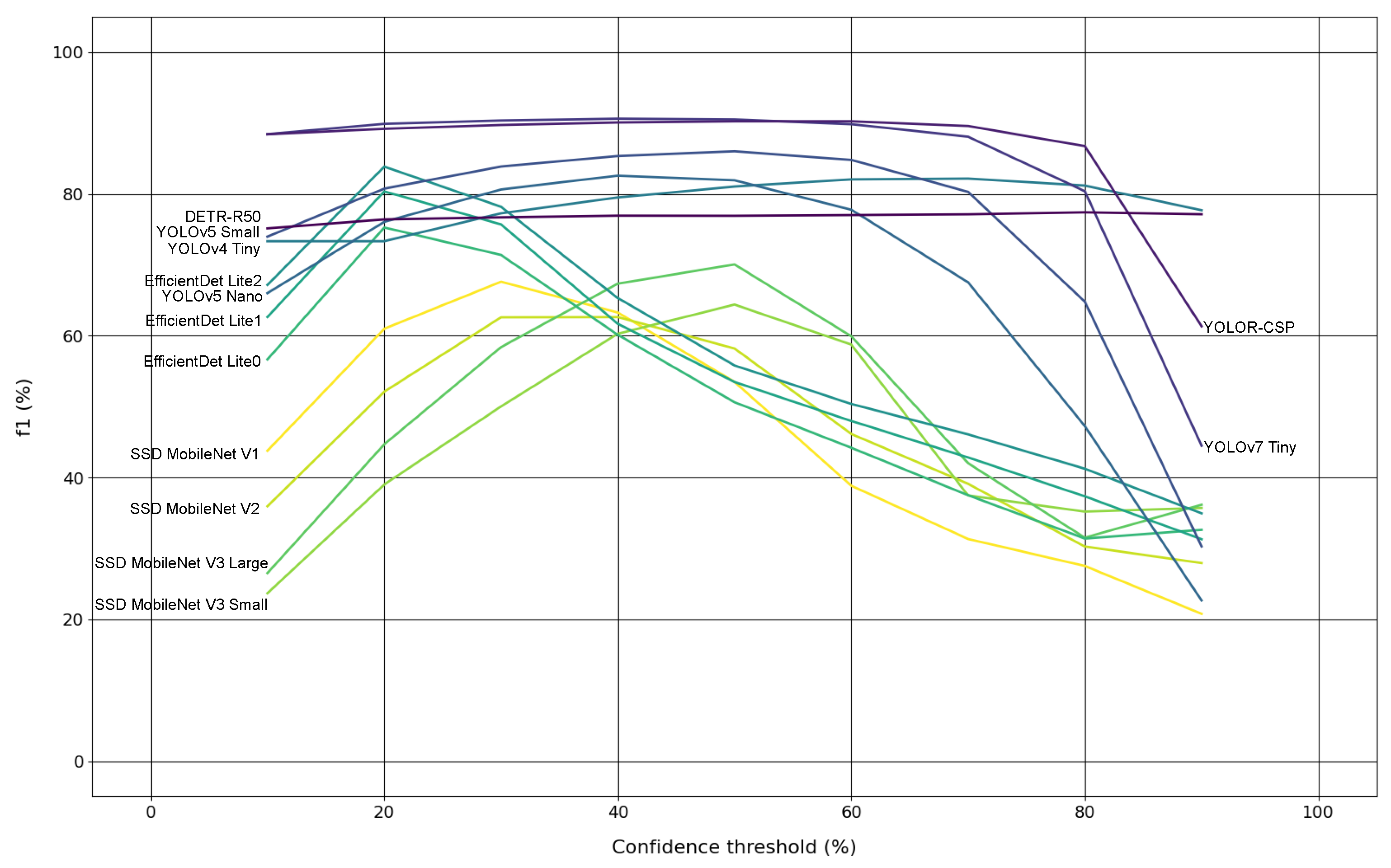
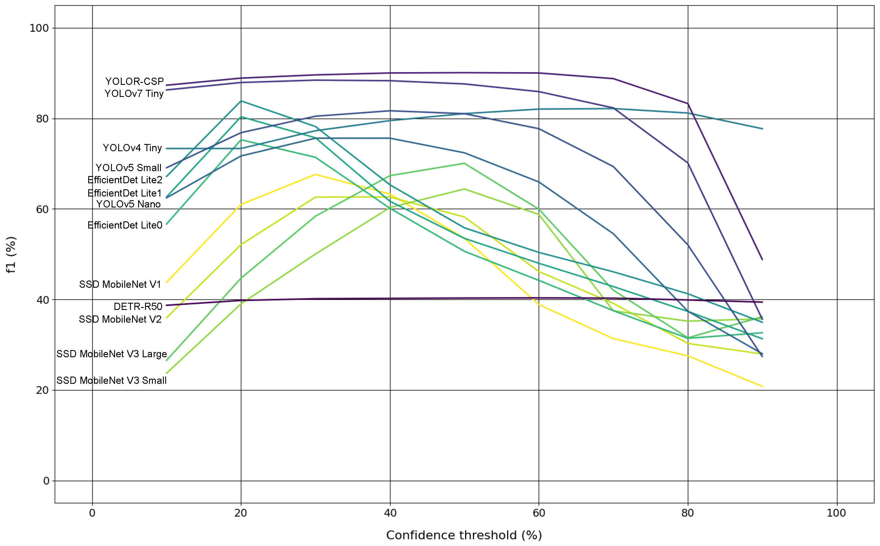
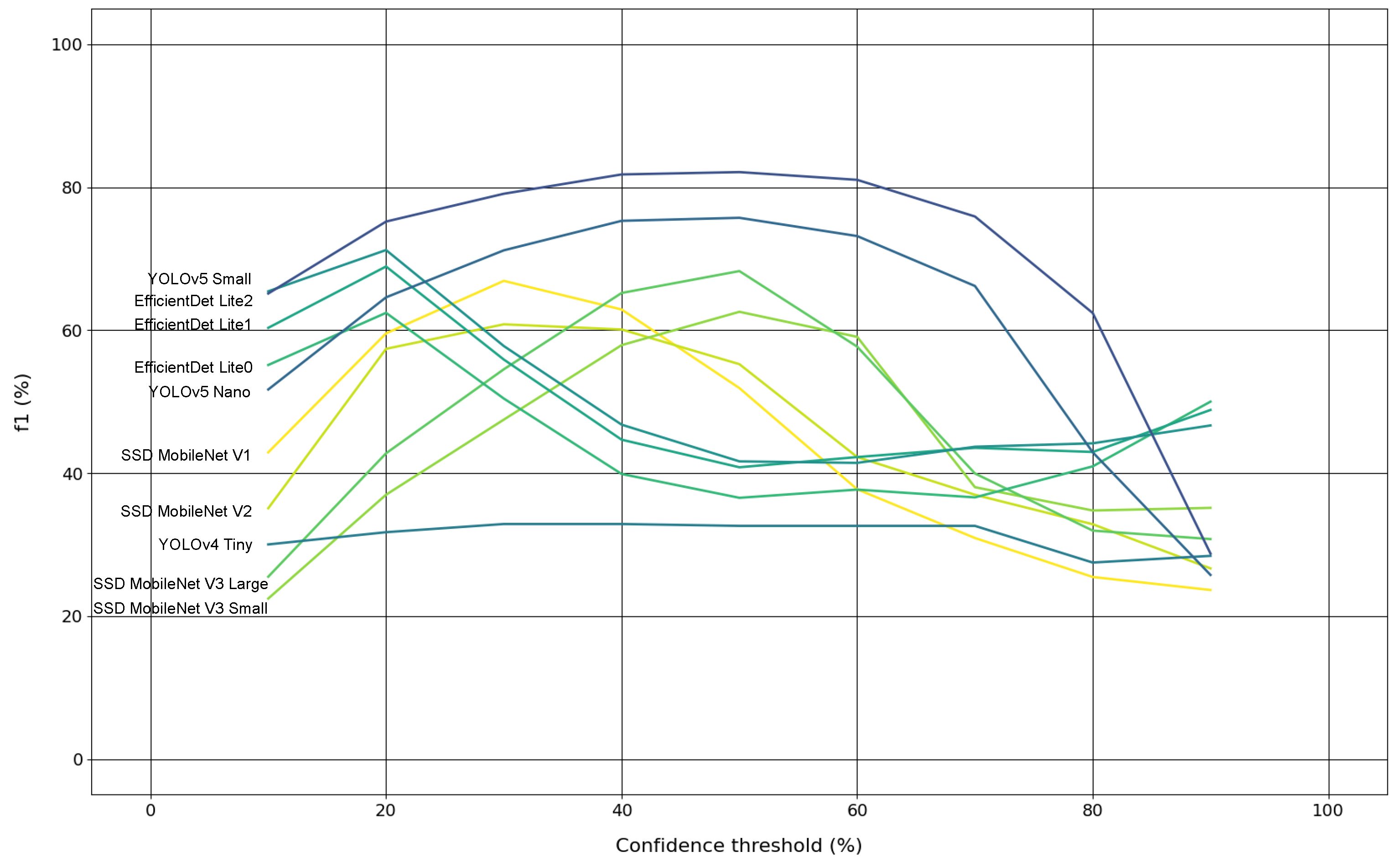
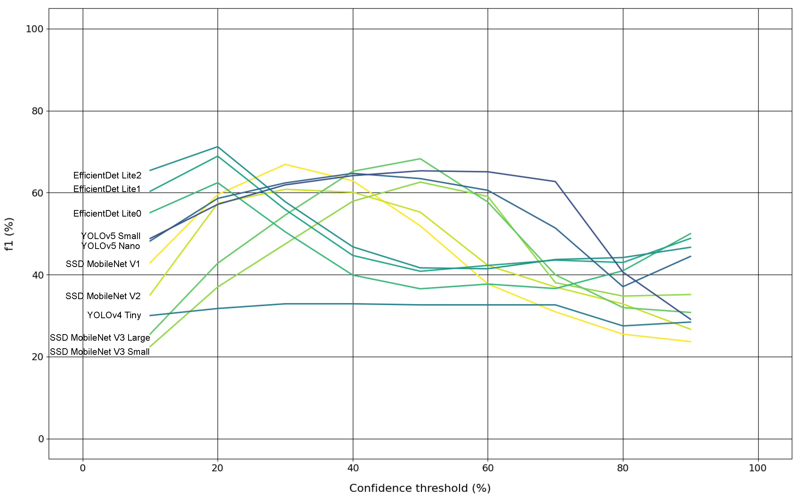
Experiment #4 is about assessing the evolution of models’ F1 scores, on the original test subset, across a confidence range from 10% to 90% with steps of 10%, producing nine confidence levels. This way, it was possible to study the most and least robust models to perform trunk detection.
Experiment #5 is about evaluating the inference speed of the models in four different edge-devices, which are defined in Table 5: Raspberry Pi 4B (CPU), Jetson Nano (GPU), Google Coral Accelerator (TPU), and NVIDIA GeForce RTX 3090 (GPU) that served as a baseline for inference speed assessing. For this experiment, the input resolutions considered for running YOLOv5, YOLOv7, YOLOR and DETR models on the CPU and TPU were 320 × 320 and 448 × 448, since these two are more constrained in terms of hardware and the second resolution is the maximum accepted by the TPU; hence, a fair comparison could be made with these two hardware. This experiment also allowed to study a field called Edge AI that has been gaining importance in recent years, where the AI data processing is completed at the edge rather than in the cloud. This type of approach enables the data to be processed in real-time, at high frame rates and at the location where it was collected [55]. This approach allows one to run algorithms on that data and collect its processing results right after.
Experiment #6 is about taking one of the 13 models, deploying it to the OAK-D edge-device (presented in the last row of 
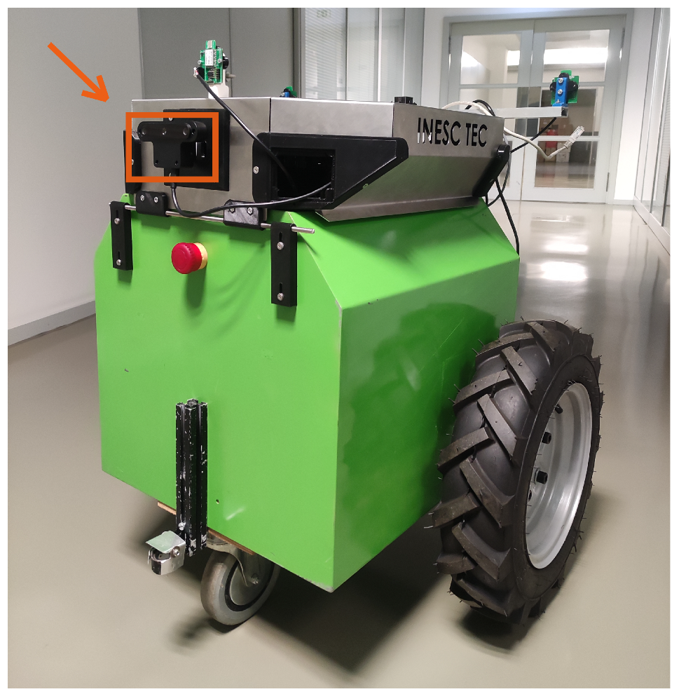
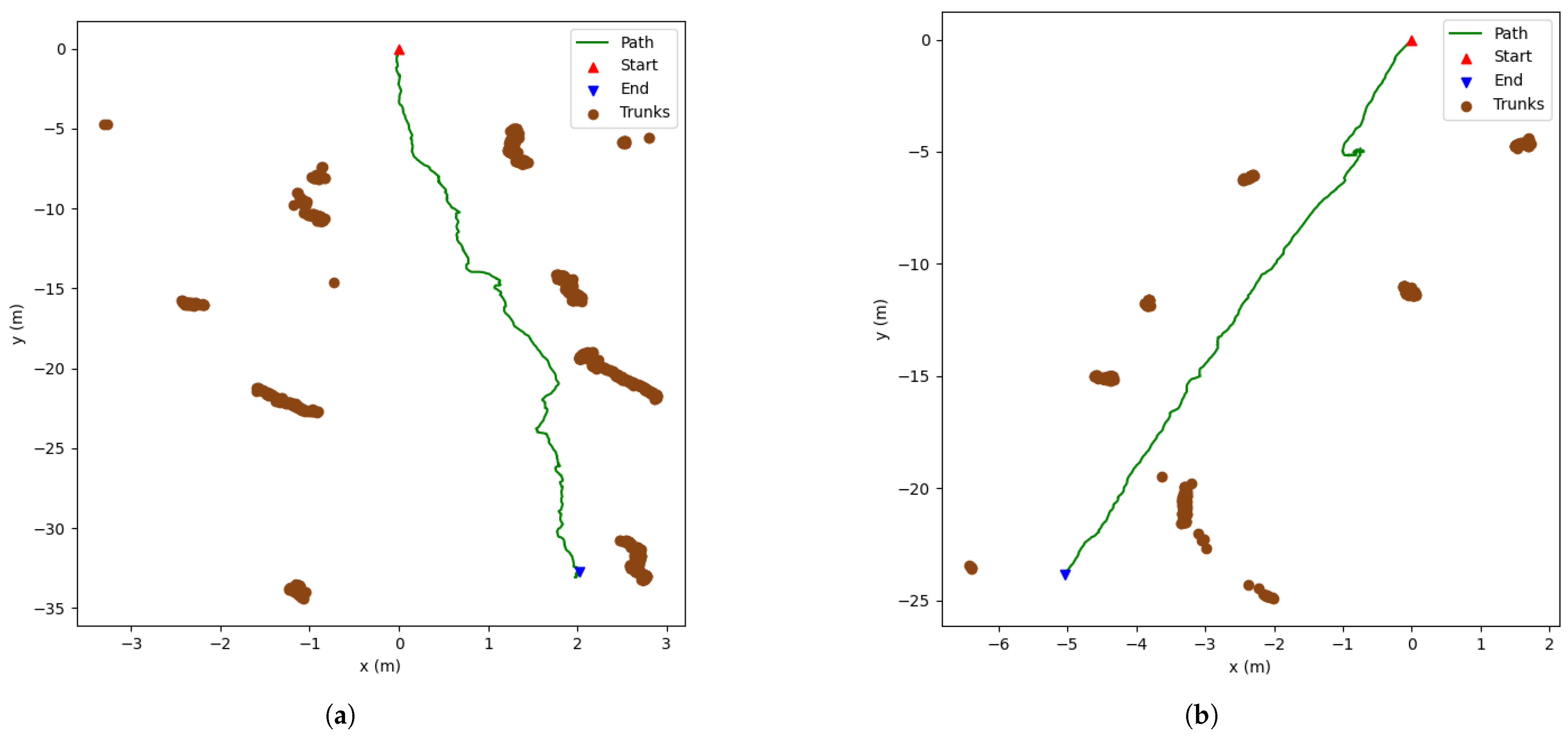
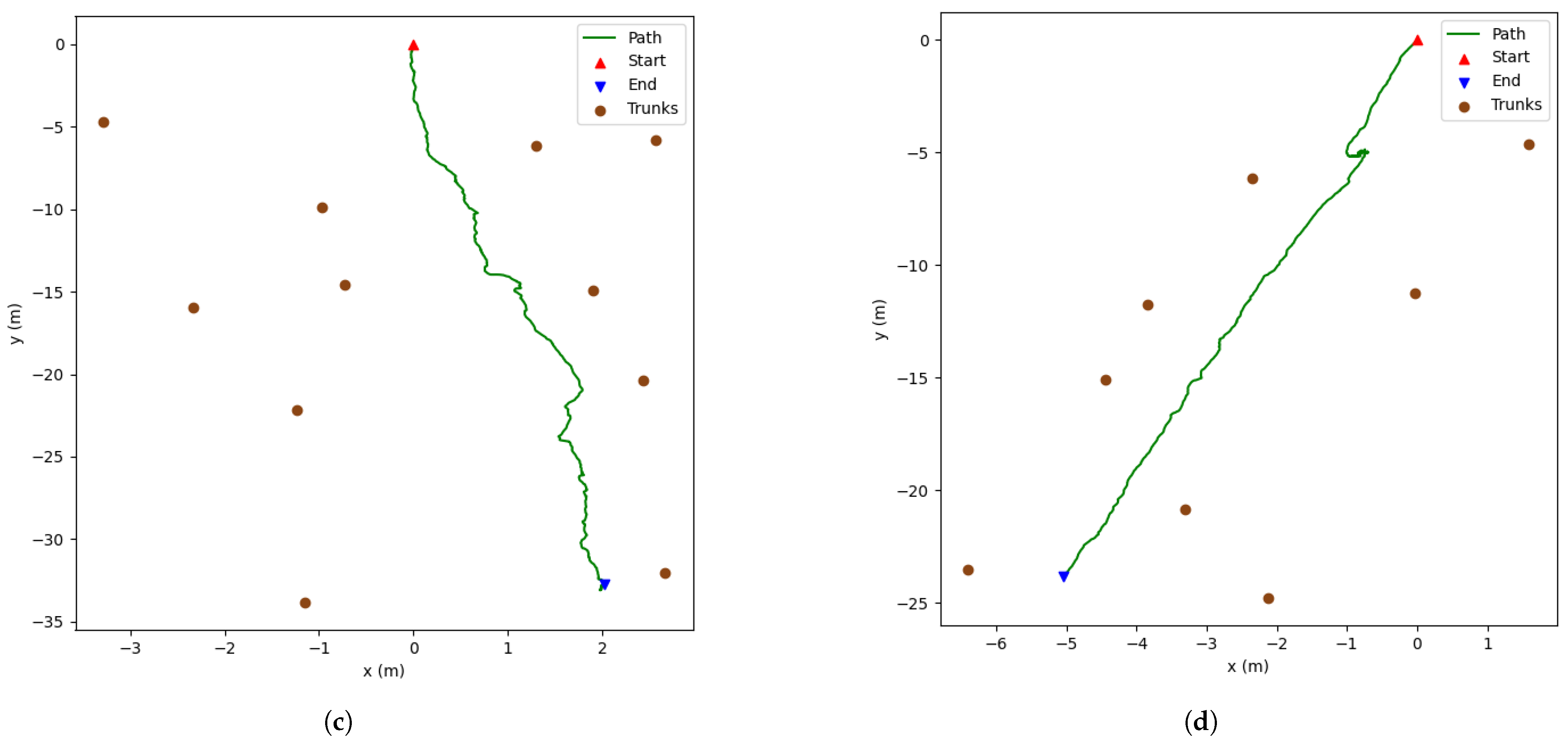
Table 5) and combining these two with a higher-level perception algorithm to map tree trunks in real-time and in a real-world context. The OAK-D was mounted on a terrestrial robotic platform as shown in Figure 3. The robot traversed a straight line twice (round trip) in an urban area that had trees with the aim of the detecting and mapping them.

4. Results

This section presents the results of the six experiments made throughout this work: the effect on the models detection accuracy when tested on augmented data; the effect on the models detection accuracy when using quantised rather than non-quantised weights; the effect on the models detection accuracy when using lower input resolutions; the evolution of the models detection accuracy over a confidence range of 10% to 90%; the models speed during inference on four edge-devices; and the deployment and running of a trunk detector on a OAK-D to map surrounding tree trunks.

4.1. Results of Experiments #1, #2 and #3—Impact of Testing Models Using Augmented Data, Impact of Quantisation and Decreasing the Input Resolution in Models’ Detection Accuracy

The results of experiment #1—presented by Table 6 and Table 7—show that in the majority of cases (about 71%), the F1 score obtained in the original test subset was higher than in the augmented one; in fact, only DETR obtained an absolute difference larger than 2%, so one may assume that the F1 score differences between the augmented and the original test subset can be considered almost irrelevant. The best non-quantised trunk detector in the original test subset, considering all input resolutions, was YOLOv7 Tiny (90.62%) with an input of 640 × 640 pixels, which was followed by YOLOR-CSP (90.41%) with 448 × 448; these two models were the best in the augmented test subset, having been tied with a 90.35% F1 score for an input of 640 × 640. On the opposite, SSD MobileNets were in general the worst non-quantised models both in the original and augmented test subsets, being only better than DETR for lower input resolutions.
With respect to experiment #2, by comparing the results of Table 6 and Table 7, one can observe that all quantised models suffered a decrease in terms of detection accuracy comparatively with their non-quantised version, and the ones that went through Post-Training Quantisation suffered more than the ones whose training was made with a Quantisation-aware approach.
From Table 6 and Table 7, one can also extract the results of experiment #3. All models whose input resolutions were tweaked (YOLOv5, YOLOv7, YOLOR and DETR) presented a detection accuracy drop, being that DETR presented the worst absolute deviations with non-quantised weights—about 9% from large (640 × 640) to medium resolution (448 × 448) and 28% from medium to small resolution (320 × 320); and YOLOv5 Small presented the worst absolute deviations with quantised weights—about 17% from 448 × 448 to 320 × 320. The model that presented minimal detection accuracy variation was YOLOR with an absolute difference below 0.5% between different resolution levels.
Figure 4 presents some examples of the detections obtained with the models when run on images belonging to the test subset. In the same figure, more specifically in Figure 4d, it is possible to verify that the models were capable of detecting objects that are tree trunks but were not annotated as ground-truth, demonstrating the knowledge gain that such models can benefit from training on larger datasets. Another clue that proves that the models performed well and remain robust even with the presence of other objects close to the tree trunks is the fact that they did not detect the person present in Figure 4a as a false positive.

4.2. Results of Experiment #4—Evolution of Detection Accuracy over Confidence Levels

The results of experiment #4, presented by Figure 5, Figure 6, Figure 7 and Figure 8, show the F1 score of the models on the original test subset—for this experiment, it was only considered the original test subset, because it was deduced, from Section 4.1, that the differences of results obtained on the augmented versus the original test subset were minimal.
The F1 score curves of the non-quantised models (with default input resolutions) for different confidence thresholds are presented in Figure 5. The same figure shows that: YOLOR and YOLOv7 are undoubtedly the best trunk detectors and have quite similar F1 score curves (their curves start only to diverge for confidences above approximately 70%); YOLOv5 Small attains F1 scores above 80% within a 20–70% confidence interval, while YOLOv5 Nano accomplished that (but with smaller values) for a shorter confidence interval of 30–55%; YOLOv4 reached quite a stable result with its curve presenting minimal to normal variation while gathering good F1 scores across different confidences, but in terms of stability, DETR was the best trunk detector, gathering F1 scores below 80% but presenting minimal variation; EfficientDet Lite models gathered similar F1 score curves (their curves follow the same evolution pattern), but, for the three of them, their accuracy drop starts at an early stage of 20% confidence; lastly, SSD MobileNet models performed worse than all models except for EfficientDet Lite models. With respect to these, SSD MobileNet V3 Small and Large presented better results from confidences within 40–65%, while SSD MobileNet V1 was only better than EfficientDet Lite0 and Lite1 within 37–50%, and SSD MobileNet V2 was better than the three EfficientDets within a 45–54% confidence range.
With respect to the evolution of F1 scores of non-quantised models but with minor resolutions for some of them (DETR, YOLOR, YOLOv7 and YOLOv5), Figure 6 shows that, in general, their curves suffered a decrease in detection accuracy, but the most notorious was DETR, whose F1 curve dropped from nearly 80% to 40%. YOLOR and YOLOv7 continue to be the best trunk detectors, but YOLOR is consistently better than YOLOv7; and YOLOv5 models are better than all EfficientDet Lites and SSD MobileNets for a confidence interval of 32–76%.
Concerning the use of quantised models for inference (on TPUs) with default input resolutions for SSD MobileNets, EfficientDet Lite and YOLOv4 Tiny models, and with maximum allowed input resolutions (448 × 448) for YOLOv5 models, Figure 7 presents the respective F1 curves across confidences. From the same figure, it can be verified that: YOLOv4 Tiny suffered the biggest F1 score drop (from 80% to 35%) comparatively to its non-quantised version; YOLOv5 models continue to perform better than EfficientDets and SSD MobileNets across the majority of confidences and, with quantised weights, YOLOv5 Small and Nano are the best trunk detectors; EfficientDet Lite models worsened their results with quantisation; and SSD MobileNets were the models that suffered less with quantisation, making them better than EfficienDets for confidence values of 30% to 70%, approximately.
The use of a minor input resolution (320 × 320) for YOLOv5 models made their F1 curves worse, as can be seen in Figure 8. However, for higher confidence values (above 60% and until nearly 80%), they continue to perform the best. For confidences between 40% and 55%, SSD MobileNet V3 Large demonstrated the best F1 score. For the remaining confidence intervals, EfficientDet Lite models attained best results.

4.3. Results of Experiment #5—Inference Times on Four Distinct Edge-Devices

Table 8 shows the inference speed results regarding experiment #5. A quick analysis indicates that the majority of the models (11 out of 13) achieve higher inference velocities (lower inference times) when performing inference on the RTX3090 GPU than on any of the other devices. For all models, except the SSD-based ones, the inference times obtained on the Raspberry Pi CPU are the worst; the SSD models obtained worst inference times on the Jetson Nano GPU. In general, for all cases, the Coral Accelerator TPU and Jetson Nano GPU were placed second and third, respectively, regarding their inference times.
Considering the four edge-devices, YOLOv4 Tiny was the fastest model overall, achieving 1.93 ms (about 518 Hz) on average when running inference on RTX3090 GPU. YOLOv7 was the second fastest model, gathering average inference speeds, also on RTX3090 GPU, between 2.5 ms (400 Hz for an input resolution of 320 × 320) and 3.5 ms (286 Hz for an input resolution of 640 × 640). The slowest model overall was YOLOR-CSP during inference on the Raspberry Pi 4 CPU with average times from 2.2 to 8.6 s in various resolutions, which was followed by DETR-ResNet50 on the same hardware (CPU) and across various resolutions with average times among 1.5 and 5.5 s. Another aspect worth mentioning is the large standard deviation values presented by SSD MobileNet V1, V2 and V3 Small on Jetson Nano. These can be explained by the use of a TensorFlow API while testing those models on Jetson Nano, which could make the inference times to vary considerably.

4.4. Results of Experiment #6—Tree Trunks Mapping

A sample of intermediary steps of the object pose estimator can be seen in Figure 9, where Figure 9a is the color image passed to the trunk detector running on OAK-D’s VPU, Figure 9b corresponds to the same color image with the tree trunk detections drawn as bounding boxes, Figure 9c is the raw depth image, and Figure 9d is the same depth image masked with the detected tree trunks. As mentioned earlier, the masked depth image enabled the pose estimation of the detected tree trunks.
The results of the tree trunks mapping experiment are shown in Figure 10. Since only raw detections were used (without any kind object matching processing), the mapping results shown in Figure 10a,b present some noise with respect to the tree trunks’ positions, which can be derived from the inaccuracies of two computational operations: the sensor pose estimation and/or the sensor’s depth estimation. These two operations are important for this task, because the first allows obtaining the distance to an object, and the second gives a relative pose of the sensor, the combination of the two enables obtaining the poses of tree trunks in relation to the sensor. So, if one of them or the two fail, the final result will present inconsistencies. As it was said before, the robot traversed a straight line trajectory, and in both Figure 10a (between y values of 15 and 25 ) and Figure 10b (between y values of 5 and 6 ), there can be noted some divergences of the expected path, which in turn cause the trunks’ positions to drift. As a minor test, we used a hierarchical clustering method on the poses of the tree trunks as a way of filtering (object matching on the XY plane) the trunk’s detections. The results of this test are shown in Figure 10c,d, where the clusters’ centroids can be observed as tree trunks. The area where this experiment was performed had nine trees to detect, so one can say that in terms of tree trunk counting, during the operation illustrated by Figure 10c, more false positives were detected (more tree trunks were detected than those that actually exist) than during the operation illustrated by Figure 10d. Additionally, OAK-D managed to produce tree trunk detections at a 23 Hz rate, while the visual–inertial odometry algorithm ran at 14 Hz, accomplishing tree trunks mapping in real-time.

5. Discussion

This section focuses on discussing the results previously presented in Section 4. From the experiments that were conducted, it is possible to affirm that: models evaluation with and without augmented data revealed little changes globally in detection accuracy level, with only one model (DETR) presenting an absolute difference on the F1 score metric larger than 2%; the impact of quantising the models weights, in order to produce inferences with them in low-cost hardware devices, is notorious since all quantised models have worsened their performance in terms of detection accuracy, and so it is the impact of decreasing the input resolution of some models, as they suffered a detection accuracy drop; the best two models overall, considering floating-point weights and default input resolutions, are YOLOR and YOLOv7 by this order, because they both presented similar F1 scores, but YOLOR seemed to be more robust and confident at detecting tree trunks, as can be seen in the results of the fourth experiment, more specifically in Figure 5 and Figure 6. The last experiment was about assessing the use of one of the models at detecting and mapping tree trunks (by means of additional algorithms); it was proven that such a task can be accomplished using only one OAK-D sensor running embedded object detection along with an object pose estimation algorithm and a sensor pose estimation algorithm.
In terms of tree trunks detection performance, this work can be compared with the one presented in [
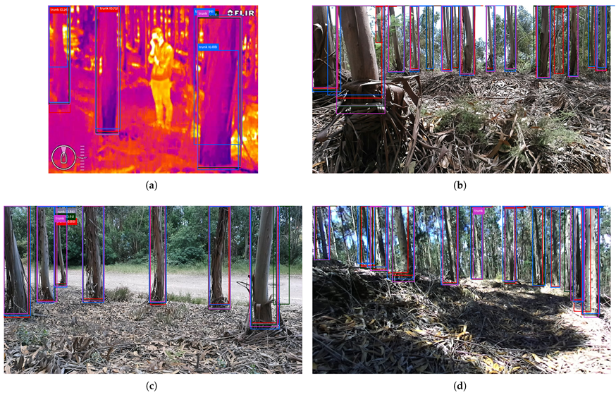
28], as the authors assessed the detection of trees at ground level, although their images were taken from the street instead of being captured in forestry locations. Despite that, by analysing our results, it can be concluded that our models showed excellent performances, as our top two—YOLOR (640 × 640) and YOLOv7 (640 × 640)—on both the original and augmented test datasets achieved F1 scores around 90%. Considering that our models were tested on an augmented test set made of by 9910 images in forestry areas, that by itself makes the detection even more difficult due to the presence of shadows (this can be seen in Figure 4d) and the existence of many more trees and more closer to each other than in the cities. Another important aspect to be highlighted is that even if the authors claim in [28] that they achieved an average precision of 98% using YOLOv2 [44] with a ResNet50 [56], their test set only had 89 images, which is around 10 times and 100 times smaller than our original and augmented test datasets, respectively. Another work to be mentioned is the one presented in [29]. In this work, the authors made use of a occlusion-aware R-CNN for detecting trees in street images. To assess the performance of their method, they used a metric called best miss rate, and they claimed to attain a 20.62% on that metric. In spite of their evaluation metric being different from the one we used, we strongly believe that our models achieved excellent detection results given that their test dataset is around 19 times smaller than our augmented test dataset. A similar work was produced in [30], where the authors proposed an object detector based on YOLOv3 [45] to detect tree trunks and telegraph/lamp posts. The authors created an original dataset composed of 812 annotated images (with 90% being trunks); then, they augmented it to obtain a 1198-image dataset, from which they picked randomly 20% of the images (198 images) to serve as the test dataset. The authors obtained the best results for an overlapping threshold of 30%, attaining an average recall rate of 90–93%, surpassing the predefined YOLOv3 architecture in best case by around 4%. Comparing to our work, besides having used a higher overlapping threshold, which makes the detection task more challenging, our augmented test dataset is much larger than theirs (around 50 times), hence proving the robustness of our models.
With respect to the tree trunk mapping, in the work proposed in [31], the authors performed stump detection and localisation in harvested forest terrains using YOLO and a ZED2 stereo camera. In fact, their object pose estimation system is similar to ours but works at a much lower rate (6.1 Hz for detection and 5.6 Hz for localisation). In fact, they mentioned the common existence of a delay when viewing the localisation results. They did not make stump mapping over an area continuously; they simply pass discrete images to their system to detect the stumps and give their estimated localisation in those images. Another aspect to be noted is that their system relies on two separate devices: a ZED camera and a GPU-based board, called NVIDIA Jetson Xavier, in order to work properly and provide perception data in real-time. On the other hand, our system only needs one OAK-D to give inertial data, coloured and depth image data, and also object detection data, that are fed, in real-time, to higher-level algorithms. Another work that aimed at mapping trees was the one presented in [27], where the authors also used a ZED2 stereo camera but instead of training DL algorithms to detect object in images (in 2D), they trained a 3D object detector to detect tree trunks in 3D data provided by the stereo camera. Then, they used the spatial mapping programming interface of the manufacturers of the stereo camera to map the detected trees in 3D space, and after, they applied a clustering method to extract only the trees from the 3D map.

6. Conclusions

This work aimed at researching forest tree trunks detection by means of Deep Learning models. To accomplish that, 13 DL-based object detection models were trained and tested using a new public dataset of manually annotated tree trunks composed by more than 5000 images. The models were evaluated in terms of detection accuracy and inference times in four different edge-devices. Then, one of the 13 models was picked and deployed to run inference in real-time on an OAK-D (AI-enabled sensor with an embedded VPU), and the obtained predictions were used to perform tree trunks mapping.
After the experiments conducted in this work, one can conclude that:
  • The use of test datasets with and without augmented data caused tiny changes in the detection accuracy level of the models, as only one model (DETR) presented an absolute difference larger than 2%;
  • The quantisation of models’ weights caused a performance worsening in all models;
  • The diminution of models’ input resolution also lowered their performances during tree trunks detection;
  • The two trunk detectors that achieved the best results were YOLOR and YOLOv7 achieving around 90% in F1 score, while YOLOR can be considered the best model overall at detecting tree trunks, as it showed more robustness and more confidence at this task, whereas the worst model was SSD MobileNet V2;
  • The fastest model overall was YOLOv4 Tiny, achieving an average inference time of 1.93 ms on NVIDIA RTX3090, while on Jetson Nano’s GPU, YOLOv5 Nano proved to be the fastest (20.21 ms); on the Raspberry Pi 4 CPU and Coral’s TPU, SSD MobileNet V3 Small (22.25 ms) and SSD MobileNet V1 (7.30 ms) were quickest, respectively;
  • Considering the trade-off between detection accuracy and detection speed, YOLOv7 is the best trunk detection model, achieving the highest F1 score similar to YOLOR with average inference times under 4 ms on the RTX3090 GPU;
  • The tree trunks mapping by means of only one sensor (OAK-D) and some higher-level estimation algorithms is possible, but it needs additional effort for filtering/matching the raw trunk detections.
This article explores several approaches to make an accelerated perception for forestry robotics. The most common approaches were compared, including processing in the vision sensor and adding dedicated hardware for processing. It is expected that the perception system presented in this work is able to improve the quality of robotic perception in a forestry environment, as the proposed strategies are most adequate to autonomous mobile robotics. As the locomotion of terrestrial robots (specially the wheeled ones) is very difficult in forests, the DL-based tree trunk detection benchmark in this work can be applied not only to terrestrial robots but also to aerial robots. However, for the latter, it is necessary for the robots to fly under the forest canopy so that the tree trunks are visible. Furthermore, the vision perception system developed in this work can be used for forest inventory purposes, such as tree counting and tree trunk diameter estimation.
Future work will include training DL models to perform the detection of different tree species and different forestry objects such as bushes, rocks and obstacles in general to increase the awareness of a robot and prevent it from getting into dangerous situations. We will aim to improve the mapping operation using embedded object detection by means of, for instance, running object tracking inside OAK-D, so instead of producing all of the object detections, only tracked objects would be outputted from the sensor. These proposals will enable further developments regarding robotic artificial vision in the forestry domain in order to achieve a more precise monitoring of the forest resources.

Author Contributions

Conceptualisation, D.Q.d.S., F.N.d.S., V.F. and A.J.S.; methodology, D.Q.d.S., F.N.d.S., V.F. and A.J.S.; software, D.Q.d.S.; validation, D.Q.d.S., F.N.d.S., V.F., A.J.S. and P.M.O.; formal analysis, D.Q.d.S. and F.N.d.S.; investigation, D.Q.d.S.; resources, D.Q.d.S. and F.N.d.S.; data curation, D.Q.d.S.; writing—original draft preparation, D.Q.d.S.; writing—review and editing, D.Q.d.S., F.N.d.S., V.F., A.J.S. and P.M.O.; visualisation, D.Q.d.S.; supervision, F.N.d.S., V.F., A.J.S. and P.M.O. All authors have read and agreed to the published version of the manuscript.

Funding

This work is financed by the ERDF—European Regional Development Fund, through the Operational Programme for Competitiveness and Internationalisation—COMPETE 2020 Programme under the Portugal 2020 Partnership Agreement, within project SMARTCUT, with reference POCI-01-0247-FEDER-048183.

Data Availability Statement

The datasets presented in this study are publicly available in Zenodo at https://doi.org/10.5281/zenodo.7186052, accessed on 11 October 2022.

Acknowledgments

Daniel Queirós da Silva thanks the FCT—Foundation for Science and Technology, Portugal for the Ph.D. Grant UI/BD/152564/2022.

Conflicts of Interest

The authors declare no conflict of interest.

Abbreviations

The following abbreviations are used in this manuscript:
AIArtificial Intelligence
APIApplication Programming Interface
CNNConvolutional Neural Network
CPUCentral Processing Unit
CSPCross Stage Partial
CVComputer Vision
DETRDEtection TRansformer
DLDeep Learning
DoFDegrees of Freedom
GBGigaByte
GNSSGlobal Navigation Satellite System
GPUGraphics Processing Unit
NMSNon-Maximum Suppression
SSDSingle Shot Detector
OPSOperations Per Second
ReLURectified Linear Unit
ROSRobot Operating System
TPUTensor Processing Unit
UAVUnmanned Aerial Vehicle
ViTVision Transformer
VPUVision Processing Unit
YOLOYou Only Look Once
YOLORYou Only Learn One Representation

References

  1. Ceccherini, G.; Duveiller, G.; Grassi, G.; Lemoine, G.; Avitabile, V.; Pilli, R.; Cescatti, A. Abrupt increase in harvested forest area over Europe after 2015. Nature 2020, 583, 72–77. [Google Scholar] [CrossRef] [PubMed]
  2. Wu, B.; Liang, A.; Zhang, H.; Zhu, T.; Zou, Z.; Yang, D.; Tang, W.; Li, J.; Su, J. Application of conventional UAV-based high-throughput object detection to the early diagnosis of pine wilt disease by deep learning. For. Ecol. Manag. 2021, 486, 118986. [Google Scholar] [CrossRef]
  3. Nguyen, H.T.; Lopez Caceres, M.L.; Moritake, K.; Kentsch, S.; Shu, H.; Diez, Y. Individual Sick Fir Tree (Abies mariesii) Identification in Insect Infested Forests by Means of UAV Images and Deep Learning. Remote Sens. 2021, 13, 260. [Google Scholar] [CrossRef]
  4. Hu, G.; Yin, C.; Wan, M.; Zhang, Y.; Fang, Y. Recognition of diseased Pinus trees in UAV images using deep learning and AdaBoost classifier. Biosyst. Eng. 2020, 194, 138–151. [Google Scholar] [CrossRef]
  5. Chiang, C.Y.; Barnes, C.; Angelov, P.; Jiang, R. Deep Learning-Based Automated Forest Health Diagnosis From Aerial Images. IEEE Access 2020, 8, 144064–144076. [Google Scholar] [CrossRef]
  6. Wang, X.; Zhao, Q.; Jiang, P.; Zheng, Y.; Yuan, L.; Yuan, P. LDS-YOLO: A lightweight small object detection method for dead trees from shelter forest. Comput. Electron. Agric. 2022, 198, 107035. [Google Scholar] [CrossRef]
  7. Li, Z.; Yang, R.; Cai, W.; Xue, Y.; Hu, Y.; Li, L. LLAM-MDCNet for Detecting Remote Sensing Images of Dead Tree Clusters. Remote Sens. 2022, 14, 3684. [Google Scholar] [CrossRef]
  8. Bo, W.; Liu, J.; Fan, X.; Tjahjadi, T.; Ye, Q.; Fu, L. BASNet: Burned Area Segmentation Network for Real-Time Detection of Damage Maps in Remote Sensing Images. IEEE Trans. Geosci. Remote Sens. 2022, 60, 1–13. [Google Scholar] [CrossRef]
  9. Cui, F. Deployment and integration of smart sensors with IoT devices detecting fire disasters in huge forest environment. Comput. Commun. 2020, 150, 818–827. [Google Scholar] [CrossRef]
  10. Fan, R.; Pei, M. Lightweight Forest Fire Detection Based on Deep Learning. In Proceedings of the 2021 IEEE 31st International Workshop on Machine Learning for Signal Processing (MLSP), Gold Coast, Australia, 25–28 October 2021; pp. 1–6. [Google Scholar] [CrossRef]
  11. Lu, K.; Xu, R.; Li, J.; Lv, Y.; Lin, H.; Liu, Y. A Vision-Based Detection and Spatial Localization Scheme for Forest Fire Inspection from UAV. Forests 2022, 13, 383. [Google Scholar] [CrossRef]
  12. Mseddi, W.S.; Ghali, R.; Jmal, M.; Attia, R. Fire Detection and Segmentation using YOLOv5 and U-NET. In Proceedings of the 2021 29th European Signal Processing Conference (EUSIPCO), Dublin, Ireland, 23–27 August 2021; pp. 741–745. [Google Scholar] [CrossRef]
  13. Ghali, R.; Akhloufi, M.A.; Jmal, M.; Mseddi, W.S.; Attia, R. Forest Fires Segmentation using Deep Convolutional Neural Networks. In Proceedings of the 2021 IEEE International Conference on Systems, Man, and Cybernetics (SMC), Melbourne, Australia, 17–20 October 2021; pp. 2109–2114. [Google Scholar] [CrossRef]
  14. Ghali, R.; Akhloufi, M.A.; Jmal, M.; Souidene Mseddi, W.; Attia, R. Wildfire Segmentation Using Deep Vision Transformers. Remote Sens. 2021, 13, 3527. [Google Scholar] [CrossRef]
  15. Wang, Z.; Peng, T.; Lu, Z. Comparative Research on Forest Fire Image Segmentation Algorithms Based on Fully Convolutional Neural Networks. Forests 2022, 13, 1133. [Google Scholar] [CrossRef]
  16. Zheng, X.; Chen, F.; Lou, L.; Cheng, P.; Huang, Y. Real-Time Detection of Full-Scale Forest Fire Smoke Based on Deep Convolution Neural Network. Remote Sens. 2022, 14, 536. [Google Scholar] [CrossRef]
  17. Oliveira, L.F.P.; Moreira, A.P.; Silva, M.F. Advances in Forest Robotics: A State-of-the-Art Survey. Robotics 2021, 10, 53. [Google Scholar] [CrossRef]
  18. Ali, W.; Georgsson, F.; Hellstrom, T. Visual tree detection for autonomous navigation in forest environment. In Proceedings of the 2008 IEEE Intelligent Vehicles Symposium, Eindhoven, The Netherlands, 4–6 June 2008; pp. 560–565. [Google Scholar] [CrossRef] [Green Version]
  19. Inoue, K.; Kaizu, Y.; Igarashi, S.; Imou, K. The development of autonomous navigation and obstacle avoidance for a robotic mower using machine vision technique. IFAC-PapersOnLine 2019, 52, 173–177. [Google Scholar] [CrossRef]
  20. Mowshowitz, A.; Tominaga, A.; Hayashi, E. Robot Navigation in Forest Management. J. Robot. Mechatron. 2018, 30, 223–230. [Google Scholar] [CrossRef]
  21. Shahria, M.T.; Rahman, A.; Zunair, H.; Aziz, S.B. Collector: A Vision-Based Semi-Autonomous Robot for Mangrove Forest Exploration and Research. In Proceedings of the 2019 International Conference on Mechatronics, Robotics and Systems Engineering (MoRSE), Bandung, Indonesia, 4–6 December 2019; pp. 207–212. [Google Scholar] [CrossRef]
  22. Zhilenkov, A.A.; Epifantsev, I.R. System of autonomous navigation of the drone in difficult conditions of the forest trails. In Proceedings of the 2018 IEEE Conference of Russian Young Researchers in Electrical and Electronic Engineering (EIConRus), Moscow and St. Petersburg, Russia, 29 January–1 February 2018; pp. 1036–1039. [Google Scholar] [CrossRef]
  23. Mannar, S.; Thummalapeta, M.; Saksena, S.K.; Omkar, S. Vision-based Control for Aerial Obstacle Avoidance in Forest Environments. IFAC-PapersOnLine 2018, 51, 480–485. [Google Scholar] [CrossRef]
  24. Dionisio-Ortega, S.; Rojas-Perez, L.O.; Martinez-Carranza, J.; Cruz-Vega, I. A deep learning approach towards autonomous flight in forest environments. In Proceedings of the 2018 International Conference on Electronics, Communications and Computers (CONIELECOMP), Cholula, Mexico, 21–23 February 2018; pp. 139–144. [Google Scholar] [CrossRef]
  25. Bergerman, M.; Billingsley, J.; Reid, J.; van Henten, E. Robotics in Agriculture and Forestry. In Springer Handbook of Robotics; Siciliano, B., Khatib, O., Eds.; Springer International Publishing: Cham, Switzerland, 2016; pp. 1463–1492. [Google Scholar] [CrossRef]
  26. Park, Y.; Shiriaev, A.; Westerberg, S.; Lee, S. 3D log recognition and pose estimation for robotic forestry machine. In Proceedings of the 2011 IEEE International Conference on Robotics and Automation, Shanghai, China, 9–13 May 2011; pp. 5323–5328. [Google Scholar] [CrossRef]
  27. Wang, B.H.; Diaz-Ruiz, C.; Banfi, J.; Campbell, M. Detecting and Mapping Trees in Unstructured Environments with a Stereo Camera and Pseudo-Lidar. In Proceedings of the 2021 IEEE International Conference on Robotics and Automation (ICRA), Xi’an, China, 30 May–5 June 2021; pp. 14120–14126. [Google Scholar] [CrossRef]
  28. Itakura, K.; Hosoi, F. Automatic Tree Detection from Three-Dimensional Images Reconstructed from 360° Spherical Camera Using YOLO v2. Remote Sens. 2020, 12, 988. [Google Scholar] [CrossRef] [Green Version]
  29. Xie, Q.; Li, D.; Yu, Z.; Zhou, J.; Wang, J. Detecting Trees in Street Images via Deep Learning with Attention Module. IEEE Trans. Instrum. Meas. 2020, 69, 5395–5406. [Google Scholar] [CrossRef]
  30. Yang, T.T.; Zhou, S.Y.; Xu, A.J. Rapid Image Detection of Tree Trunks Using a Convolutional Neural Network and Transfer Learning. IAENG Int. J. Comput. Sci. 2021, 48, 1–8. [Google Scholar]
  31. Li, S.; Lideskog, H. Implementation of a System for Real-Time Detection and Localization of Terrain Objects on Harvested Forest Land. Forests 2021, 12, 1142. [Google Scholar] [CrossRef]
  32. Fortin, J.M.; Gamache, O.; Grondin, V.; Pomerleau, F.; Giguère, P. Instance Segmentation for Autonomous Log Grasping in Forestry Operations. arXiv 2022, arXiv:2203.01902. [Google Scholar]
  33. Liu, W.; Anguelov, D.; Erhan, D.; Szegedy, C.; Reed, S.; Fu, C.Y.; Berg, A.C. SSD: Single Shot MultiBox Detector. In Lecture Notes in Computer Science; Springer: Berlin/Heidelberg, Germany, 2016; pp. 21–37. [Google Scholar] [CrossRef] [Green Version]
  34. Howard, A.G.; Zhu, M.; Chen, B.; Kalenichenko, D.; Wang, W.; Weyand, T.; Andreetto, M.; Adam, H. MobileNets: Efficient Convolutional Neural Networks for Mobile Vision Applications. arXiv 2017, arXiv:1704.04861. [Google Scholar]
  35. Sandler, M.; Howard, A.; Zhu, M.; Zhmoginov, A.; Chen, L.C. MobileNetV2: Inverted Residuals and Linear Bottlenecks. In Proceedings of the IEEE Conference on Computer Vision and Pattern Recognition (CVPR), Salt Lake City, UT, USA, 18–22 June 2018. [Google Scholar]
  36. Howard, A.; Sandler, M.; Chu, G.; Chen, L.C.; Chen, B.; Tan, M.; Wang, W.; Zhu, Y.; Pang, R.; Vasudevan, V.; et al. Searching for MobileNetV3. In Proceedings of the IEEE/CVF International Conference on Computer Vision, Seoul, Republic of Korea, 27 October–2 November 2019. [Google Scholar]
  37. Tan, M.; Pang, R.; Le, Q.V. EfficientDet: Scalable and Efficient Object Detection. In Proceedings of the 2020 IEEE/CVF Conference on Computer Vision and Pattern Recognition (CVPR), Seattle, WA, USA, 13–19 June 2020; pp. 10778–10787. [Google Scholar] [CrossRef]
  38. Bochkovskiy, A.; Wang, C.Y.; Liao, H.Y.M. YOLOv4: Optimal Speed and Accuracy of Object Detection. arXiv 2020, arXiv:2004.10934. [Google Scholar]
  39. Wang, C.Y.; Bochkovskiy, A.; Liao, H.Y.M. YOLOv7: Trainable bag-of-freebies sets new state-of-the-art for real-time object detectors. arXiv 2022, arXiv:2207.02696. [Google Scholar] [CrossRef]
  40. Wang, C.Y.; Mark Liao, H.Y.; Wu, Y.H.; Chen, P.Y.; Hsieh, J.W.; Yeh, I.H. CSPNet: A New Backbone that can Enhance Learning Capability of CNN. In Proceedings of the 2020 IEEE/CVF Conference on Computer Vision and Pattern Recognition Workshops (CVPRW), Seattle, WA, USA, 14–19 June 2020; pp. 1571–1580. [Google Scholar] [CrossRef]
  41. Wang, C.Y.; Yeh, I.H.; Liao, H.Y.M. You Only Learn One Representation: Unified Network for Multiple Tasks. arXiv 2021, arXiv:2105.04206. [Google Scholar] [CrossRef]
  42. Carion, N.; Massa, F.; Synnaeve, G.; Usunier, N.; Kirillov, A.; Zagoruyko, S. End-to-End Object Detection with Transformers. In Proceedings of the Computer Vision—ECCV 2020; Vedaldi, A., Bischof, H., Brox, T., Frahm, J.M., Eds.; Springer International Publishing: Cham, Switzerland, 2020; pp. 213–229. [Google Scholar]
  43. Redmon, J.; Divvala, S.; Girshick, R.; Farhadi, A. You only look once: Unified, real-time object detection. In Proceedings of the IEEE Computer Society Conference on Computer Vision and Pattern Recognition, Las Vegas, NV, USA, 27–30 June 2016; pp. 779–788. [Google Scholar] [CrossRef] [Green Version]
  44. Redmon, J.; Farhadi, A. YOLO9000: Better, faster, stronger. In Proceedings of the 30th IEEE Conference on Computer Vision and Pattern Recognition, CVPR 2017, Honolulu, HI, USA, 21–26 July 2017; pp. 6517–6525. [Google Scholar] [CrossRef] [Green Version]
  45. Redmon, J.; Farhadi, A. YOLO v.3. Technical Report, University of Washington. 2018. Available online: https://pjreddie.com/media/files/papers/YOLOv3.pdf (accessed on 26 July 2022).
  46. Li, C.; Li, L.; Jiang, H.; Weng, K.; Geng, Y.; Li, L.; Ke, Z.; Li, Q.; Cheng, M.; Nie, W.; et al. YOLOv6: A Single-Stage Object Detection Framework for Industrial Applications. arXiv 2022, arXiv:2209.02976. [Google Scholar] [CrossRef]
  47. Lin, T.Y.; Maire, M.; Belongie, S.; Hays, J.; Perona, P.; Ramanan, D.; Dollár, P.; Zitnick, C.L. Microsoft COCO: Common Objects in Context. In Proceedings of the Computer Vision—ECCV 2014; Fleet, D., Pajdla, T., Schiele, B., Tuytelaars, T., Eds.; Springer International Publishing: Cham, Switzerland, 2014; pp. 740–755. [Google Scholar]
  48. Dosovitskiy, A.; Beyer, L.; Kolesnikov, A.; Weissenborn, D.; Zhai, X.; Unterthiner, T.; Dehghani, M.; Minderer, M.; Heigold, G.; Gelly, S.; et al. An Image is Worth 16 × 16 Words: Transformers for Image Recognition at Scale. In Proceedings of the 9th International Conference on Learning Representations, ICLR 2021, Virtual Event, Austria, 3–7 May 2021. [Google Scholar]
  49. Da Silva, D.Q.; dos Santos, F.N.; Sousa, A.J.; Filipe, V. Visible and Thermal Image-Based Trunk Detection with Deep Learning for Forestry Mobile Robotics. J. Imaging 2021, 7, 176. [Google Scholar] [CrossRef]
  50. Da Silva, D.Q.; dos Santos, F.N.; Sousa, A.J.; Filipe, V.; Boaventura-Cunha, J. Unimodal and Multimodal Perception for Forest Management: Review and Dataset. Computation 2021, 9, 127. [Google Scholar] [CrossRef]
  51. Everingham, M.; Gool, L.V.; Williams, C.K.I.; Winn, J.; Zisserman, A. The Pascal Visual Object Classes (VOC) Challenge. Int. J. Comput. Vis. 2010, 88, 303–338. [Google Scholar] [CrossRef] [Green Version]
  52. Geneva, P.; Eckenhoff, K.; Lee, W.; Yang, Y.; Huang, G. OpenVINS: A Research Platform for Visual-Inertial Estimation. In Proceedings of the 2020 IEEE International Conference on Robotics and Automation (ICRA), Paris, France, 31 May–31 August 2020; pp. 4666–4672. [Google Scholar] [CrossRef]
  53. Shorten, C.; Khoshgoftaar, T. A survey on Image Data Augmentation for Deep Learning. J. Big Data 2019, 6, 60. [Google Scholar] [CrossRef]
  54. Gholami, A.; Kim, S.; Zhen, D.; Yao, Z.; Mahoney, M.; Keutzer, K. A Survey of Quantization Methods for Efficient Neural Network Inference. In Low-Power Computer Vision; Chapman and Hall/CRC: New York, NY, USA, 2022; pp. 291–326. [Google Scholar] [CrossRef]
  55. Aguiar, A.S.; Monteiro, N.N.; Santos, F.N.d.; Solteiro Pires, E.J.; Silva, D.; Sousa, A.J.; Boaventura-Cunha, J. Bringing Semantics to the Vineyard: An Approach on Deep Learning-Based Vine Trunk Detection. Agriculture 2021, 11, 131. [Google Scholar] [CrossRef]
  56. He, K.; Zhang, X.; Ren, S.; Sun, J. Deep Residual Learning for Image Recognition. In Proceedings of the 2016 IEEE Conference on Computer Vision and Pattern Recognition (CVPR), Las Vegas, NV, USA, 27–30 June 2016; pp. 770–778. [Google Scholar] [CrossRef]
Figure 1. OAK-D sensing device accommodates an embedded inertial measurement sensor and three cameras: a monochromatic stereo-vision pair and central coloured camera. This figure is from: https://docs.luxonis.com/projects/hardware/en/latest/pages/BW1098OAK.html, accessed on 26 July 2022.
Robotics 11 00136 g001
Figure 2. Tree trunk mapping algorithm diagram: green blocks are data provided by sensors, yellow blocks are computational data, blue blocks are computational nodes, and purple blocks are results. The computational nodes have been developed in ROS2, of which, one of them computes the detected object XYZ pose, the other corresponds to a visual–inertial odometry algorithm that estimates the sensor’s six DoF poses, and the last one uses the information given by the latter two and maps the detected objects.
Robotics 11 00136 g002
Figure 3. Robotic platform with OAK-D (surrounded by an orange rectangle).
Robotics 11 00136 g003
Figure 4. Trunk detections in some example test images: the pink bounding boxes are ground-truth while the others are detections obtained from trained models: (a) detections in FLIR’s thermal image, (b) detections in OAK-D’s color image, (c) detections in OAK-D’s color image, (d) detections in ZED’s color image.
Robotics 11 00136 g004
Figure 5. Evolution of F1 score of the non-quantised models, with their default input resolutions, over several confidence thresholds.
Robotics 11 00136 g005
Figure 6. Evolution of F1 score of the non-quantised models, with minor input resolutions, over several confidence thresholds.
Robotics 11 00136 g006
Figure 7. Evolution of F1 score of the quantised models, with maximum input resolutions, over several confidence thresholds.
Robotics 11 00136 g007
Figure 8. Evolution of F1 score of the quantised models, with minor input resolutions, over several confidence thresholds.
Robotics 11 00136 g008
Figure 9. Results of the distance estimation to the tree trunks by means of depth information: (a) color image, (b) color image with detected tree trunks, (c) depth image, (d) depth image with detected tree trunks and their estimated distances.
Robotics 11 00136 g009
Figure 10. Trunk mapping results: (a,b) are the mapping results without tree trunk clustering, (c,d) are the mapping results with tree trunk clustering.
Robotics 11 00136 g010aRobotics 11 00136 g010b
Table 1. Features of the original dataset images.
CameraResolution (Width × Height)SpectrumFootage Location# Images
FLIR M232640 × 512ThermalLobão, Valongo866, 940
ZED Stereo1280 × 720VisibleValongo1487
Allied Mako G-1251292 × 964VisibleVila do Conde467
OAK-D1280 × 720VisibleValongo850
GoPro Hero61920 × 1080VisibleLobão715
Table 2. Augmentation operations applied to the original images.
OperationValueDescription
BlurRandomBlur the image
Flip-Flip the image horizontally
Hue and SaturationRandomChange image’s hue and saturation levels
ContrastRandomChange image’s contrast level
NoiseRandomGaussian noise addition
Rotation−15 Rotate image −15
Rotation+15 Rotate image +15
Scale0.7×Scale the image by 0.7
Scale1.3×Scale the image by 1.3
Table 3. Training parameters of the Deep Learning models.
ModelInput ResolutionLearning RateBatch SizeEpochs
SSD MobileNet V1300 × 3000.00232130
SSD MobileNet V2300 × 3000.0023280
SSD MobileNet V3 Small320 × 3200.00232130
SSD MobileNet V3 Large320 × 3200.0023265
EfficientDet Lite0320 × 3200.086470
EfficientDet Lite1384 × 3840.086470
EfficientDet Lite2448 × 4480.086470
YOLOv4 Tiny416 × 4160.0026474
YOLOv5 Nano640 × 6400.013250
YOLOv5 Small640 × 6400.013250
YOLOv7 Tiny640 × 6400.0132100
YOLOR-CSP640 × 6400.0028100
DETR-ResNet501333 × 1333 *0.00018200
Table 4. Quantisation results with the number of supported and unsupported operations of each model to run on the TPU.
ModelSupported OperationsUnsupported OperationsRatio of Supported Operations
SSD MobileNet V173396%
SSD MobileNet V2108397%
SSD MobileNet V3 Small1385770%
SSD MobileNet V3 Large1505573%
EfficientDet Lite0264399%
EfficientDet Lite1319399%
EfficientDet Lite2354399%
YOLOv4 Tiny41491%
YOLOv5 Nano2560100%
YOLOv5 Small2550100%
Table 5. Specifications of the hardware platforms to perform Deep Learning inference.
Processing UnitNamePlatformMemory (GB)Compute Capability (OPS × 10 12 )
CPUQuad core Cortex-A72 (ARM v8)Raspberry Pi 4B40.0135 (float)
GPU10496-core NVIDIA GeForce RTX 3090Desktop computer2435 (float)
GPU128-core NVIDIA MaxwellJetson Nano20.472 (float)
TPUGoogle Edge TPU co-processorCoral USB Accelerator-4 (int8)
VPUIntel Movidius Myriad XOAK-D-1.4 (float)
Table 6. Detection results in the original and augmented datasets with variable resolutions for some models and non-quantised weights. For each dataset, the best F1 score is in bold, and the worst is in italic.
ModelInput ResolutionBest F1
OriginalAugmented
SSD MobileNet V1300 × 30067.62%67.78%
SSD MobileNet V2300 × 30062.63%61.47%
SSD MobileNet V3 Small320 × 32064.39%64.63%
SSD MobileNet V3 Large320 × 32070.06%69.91%
EfficientDet Lite0320 × 32075.27%74.63%
EfficientDet Lite1384 × 38480.36%79.98%
EfficientDet Lite2448 × 44883.85%83.00%
YOLOv4 Tiny416 × 41682.16%81.50%
YOLOv5 Nano640 × 64082.58%80.81%
448 × 44880.85%79.55%
320 × 32075.62%74.67%
YOLOv5 Small640 × 64086.02%85.17%
448 × 44885.75%84.75%
320 × 32081.67%81.01%
YOLOv7 Tiny640 × 64090.62%90.35%
448 × 44890.18%89.64%
320 × 32088.45%87.51%
YOLOR-CSP640 × 64090.26%90.35%
448 × 44890.41%90.33%
320 × 32090.10%90.02%
DETR-ResNet50640 × 64077.41%76.62%
448 × 44868.29%67.88%
320 × 32040.33%44.20%
Table 7. Detection results in the original and augmented datasets with quantised weights and minor resolutions for YOLOv5 models. For each dataset, the best F1 score is in bold and the worst is in italic.
ModelInput ResolutionBest F1
OriginalAugmented
SSD MobileNet V1300 × 30066.90%66.63%
SSD MobileNet V2300 × 30060.82%59.52%
SSD MobileNet V3 Small320 × 32062.57%63.50%
SSD MobileNet V3 Large320 × 32068.27%68.54%
EfficientDet Lite0320 × 32062.42%63.26%
EfficientDet Lite1384 × 38468.91%69.26%
EfficientDet Lite2448 × 44871.21%71.23%
YOLOv4 Tiny416 × 41632.87%32.41%
YOLOv5 Nano448 × 44875.72%74.84%
320 × 32064.70%64.63%
YOLOv5 Small448 × 44882.12%81.86%
320 × 32065.32%66.24%
Table 8. Inference time (in ms) results in different processing units: one TPU, one CPU and two GPUs. For each edge-device, the lowest time is in bold, and the highest is in italic.
ModelInput ResolutionEdge-Devices
GPUGPUCPUTPU
RTX3090Jetson NanoRaspberry Pi 4Coral Accelerator
SSD MobileNet V1300 × 300 7.43 ± 0.71 149.53 ± 505.14 58.42 ± 5.80 7.30 ± 0.48
SSD MobileNet V2300 × 300 9.92 ± 1.10 180.41 ± 358.27 60.50 ± 5.03 8.64 ± 0.55
SSD MobileNet V3 Small320 × 320 11.80 ± 1.32 153.55 ± 783.15 22.25 ± 3.19 53.11 ± 5.41
SSD MobileNet V3 Large320 × 320 12.71 ± 1.29 139.76 ± 40.33 57.10 ± 5.28 104.03 ± 8.71
EfficientDet Lite0320 × 320 16.89 ± 1.76 —– 176.43 ± 29.98 27.09 ± 2.08
EfficientDet Lite1384 × 384 18.23 ± 1.88 —– 321.09 ± 13.44 40.03 ± 2.92
EfficientDet Lite2448 × 44818.76 ± 1.98—– 532.25 ± 17.66 68.16 ± 2.95
YOLOv4 Tiny416 × 4161.93 ± 0.07 34.96 ± 0.46 470.40 ± 9.71 9.19 ± 0.50
YOLOv5 Nano640 × 640 5.40 ± 0.30 42.91 ± 0.35 284.06 ± 34.18 —–
448 × 448 5.32 ± 0.28 22.99 ± 0.80 129.07 ± 10.59 20.22 ± 0.37
320 × 320 5.24 ± 0.29 20.21 ± 3.01 61.79 ± 4.87 10.98 ± 0.39
YOLOv5 Small640 × 640 5.47 ± 0.24 110.04 ± 2.18 974.57 ± 44.39 —–
448 × 448 5.48 ± 0.31 54.54 ± 0.29 463.48 ± 14.28 43.75 ± 0.71
320 × 320 5.44 ± 0.26 31.01 ± 0.23 233.68 ± 30.57 19.08 ± 0.64
YOLOv7 Tiny640 × 640 3.50 ± 0.13 90.14 ± 2.19 988.79 ± 9.12 —–
448 × 448 2.91 ± 0.07 44.82 ± 0.14 506.53 ± 2.95 —–
320 × 320 2.50 ± 0.15 25.29 ± 0.19 268.88 ± 11.08 —–
YOLOR-CSP640 × 640 12.03 ± 0.18 616.09 ± 9.178652.50 ± 49.77—–
448 × 448 7.72 ± 0.07 300.89 ± 7.25 4720.24 ± 15.52 —–
320 × 320 6.12 ± 0.06 178.89 ± 0.53 2201.46 ± 18.69 —–
DETR-ResNet50640 × 640 8.43 ± 0.29 453.07 ± 48.11 5568.48 ± 20.22 —–
448 × 448 6.14 ± 0.29 228.84 ± 5.09 2863.37 ± 10.68 —–
320 × 320 4.83 ± 0.25 143.73 ± 9.87 1520.74 ± 9.37 —–
Publisher’s Note: MDPI stays neutral with regard to jurisdictional claims in published maps and institutional affiliations.

