Article

Benchmarking Dynamic Balancing Controllers for Humanoid Robots

by
Juan A. Castano
1,*,
Joseph Humphreys
2,
Enrico Mingo Hoffman
3,
Noelia Fernández Talavera
1,
Maria Cristina Rodriguez Sanchez
1 and
Chengxu Zhou
2,*
1
Department of Applied Mathematics, Science and Material Engineering, and Electronics Technologies, School of Experimental Sciences and Technology, Campus de Mostoles, King Juan Carlos University, 28933 Madrid, Spain
2
Faculty of Engineering and Physical Sciences, School of Mechanical Engineering, University of Leeds, Leeds LS2 9JT, UK
3
PAL Robotics, 08005 Barcelona, Spain
*
Authors to whom correspondence should be addressed.
Robotics 2022, 11(5), 114; https://doi.org/10.3390/robotics11050114
Submission received: 8 September 2022 / Revised: 4 October 2022 / Accepted: 16 October 2022 / Published: 19 October 2022
(This article belongs to the Special Issue Legged Robots into the Real World)

Abstract

:
This paper presents a comparison study of three control design approaches for humanoid balancing based on the Center of Mass ( C o M ) stabilization and body posture adjustment. The comparison was carried out under controlled circumstances allowing other researchers to replicate and compare our results with their own. The feedback control from state space design is based on simple models and provides sufficient robustness to control complex and high Degrees of Freedom (DoFs) systems, such as humanoids. The implemented strategies allow compliant behavior of the robot in reaction to impulsive or periodical disturbances, resulting in a smooth and human-like response while considering constraints. In this respect, we implemented two balancing strategies to compensate for the C o M deviation. The first one uses the robot’s capture point as a stability principle and the second one uses the Force/Torque sensors at the ankles to define a C o M reference that stabilizes the robot. In addition, was implemented a third strategy based on upper body orientation to absorb external disturbances and counterbalance them. Even though the balancing strategies are implemented independently, they can be merged to further increase balancing performance. The proposed strategies were previously applied on different humanoid bipedal platforms, however, their performance could not be properly benchmarked before. With this concern, this paper focuses on benchmarking in controlled scenarios to help the community in comparing different balance techniques. The key performance indicators (KPIs) used in our comparison are the C o M deviation, the settling time, the maximum measured orientation, passive gait measure, measured ankles torques, and reconstructed Center of Pressure ( C o P ). The benchmarking experiments were carried out in simulations and using the facility at Istituto Italiano di Tecnologia on the REEM-C humanoid robot provided by PAL robotics inside the EU H2020 project EUROBENCH framework.

1. Introduction

In the study of biped locomotion, specific attention has been given to the balance of humanoid robots, being a fundamental prerequisite for the secure performance of robots deployed in real environments. However, it is necessary to consider different balancing strategies for different perturbations, particularly when a natural and safe interaction with the environment is required. In this case, the energy added to the system by interactions should be damped [1] producing a compliant response of the system that is more secure for human interaction. Thus, balance controllers should provide a soft and reliable response by continuous adaptation of the control action, depending on the robot’s state. On the other hand, when impulsive or soft continuous perturbations are introduced, more rigid behaviors should counterbalance such disturbances.
Different balancing strategies have been introduced in the state of the art, for instance, [2,3,4,5] among others. In [6], an ankle balancing strategy, where the Linear Inverted Pendulum Model (LIPM) augmented with virtual spring dampers, is used to generate a compliant response against external disturbances. Furthermore, in [7] springs are added to the model to provide compliant behavior. Furthermore, this work developed a hip bending balancing strategy using a three-link planar model of the robot, utilizing the joints located in the ankle and the hip.
Two different balancing methods were presented in [8]. In accordance with the external disturbance, the humanoid robot applies an ankle strategy or a hip-bending strategy. In the first case, a torque is applied at the ankles to absorb the forces caused by an external push. In the second case, the robot bends the body to absorb the impact and change the C o M position, keeping the Center of Pressure ( C o P ) inside the desired stability margins. In this work, the C o P principle provides the stability criterion, and the humanoid is modeled as a planar double inverted pendulum that is controlled by an Linear-Quadratic Regulator (LQR) controller. Therefore, constraints can be handled with a clipping strategy using the limit value. The integration of these approaches depends on an external gain that maps the disturbance with the appropriate strategy.
In [9], the center of gravity and the Zero Moment Point (ZMP) are used to implement a balancing strategy. The authors use the ZMP stability criterion as a constraint to guarantee the stability of the humanoid [10] while modeling the dynamics through the inverted pendulum model. The ZMP has been validated as an effective stability criterion, seeing much use within control strategies [11,12,13].
To ensure balance, the ZMP should remain inside the support polygon of the humanoid so that the robot does not tip about the stance foot [11]. It is worth noting that the C o P and ZMP coincide when the robot only has its feet in contact on flat terrain.
In the balancing of humanoids, there is a necessity for a soft transition between ankle and hip bending strategies. The work in [3] presents a smooth transition of the balancing strategies by applying a spline function integrated with a proportional controller. Another work that combines the ankle and hip strategies is [14]. In this work, the authors formulate the control to reject external disturbances using the ankle strategy for soft disturbances or the hip bending strategy for stronger ones. In both cases, the stability conditions are based on the ZMP criterion.
Overall, many different balancing strategies have been developed. However, their performance can not be compared directly since their implementation is drastically different from one another. This leaves researchers with the challenging question of which control strategy to use based on their requirements, with no parameterized method to do so.
To provide a general and comprehensive tool answer to this question, in this work first, we implement three different balancing strategies in the REEM-C humanoid robot from PAL Robotics, of which a model is available online; therefore, simulation studies can be replicated. This hardware was provided under the EUROBENCH project. Secondly, we test the selected balancing strategies in a simulated scenario for impulsive and quasi-static disturbances. This was performed considering the test bed develop under the DYSTURBANCE [15] Third FSTPs (Financial Support to Third Party, provided by EUROBENCH) project. Thirdly, we performed experimentation in the real REEM-C platform using the test beds available at the Humanoids Testing Facility at the Istituto Italiano di Tecnologia. We performed experimentation on the REEM-C platform for the different balancing strategies under impulsive and quasi-static perturbation. This way simulation and experimental results can be contrasted. Finally, we summarize the obtained results considering different Key Performance Indicators (KPI), allowing performance comparison over different variables. In this way, we provide the community with comparable data over the method selection and allow other teams to compare their own balancing controllers with the ones given in this work.
Regarding the used methods, two methods compensated for the C o M deviation proposed in [16,17,18] and a third one for the orientation of the robot [16,19]. The cooperative behavior of individual strategies is obtained by proper compensation of the given strategies considering the robot’s structure so that no additional controllers or gains are required for a smooth transition, and both stabilizers cooperate permanently.
The first balancing strategy [16] uses the Capture Point ( C P ) as a stability criterion and generates a horizontal displacement of the C o M , dissipating the injected energy to the system while achieving a compliant response. This strategy considers the single-mass model to generate the desired response.
The second strategy [17,18] introduces a virtual spring-damper system at the robot C o M level to generate compliant responses to deal with unexpected disturbances caused by modeling discrepancies or unforeseen interactions such as early or late foot landings.
The third strategy [19] allows the system to dissipate energy by an attitude controller based on the free rotational body model. This strategy dissipates the additional energy by rotating the upper body of the humanoid.
Even though stabilizing strategies can be based on simple PID or LQR controllers [16], in this work, two of the three presented methodologies use Model Predictive Control (MPC), being well-accepted in academia and the industry. In particular, we exploited the Robust Extended Predictive Self-Adaptive Control (R-EPSAC) approach [20].
To assess the performance of the proposed balancing strategies, we perform a series of experiments on a full-size humanoid robot the REEM-C, designed and manufactured by PAL Robotics, at the EUROBENCH (https://eurobench2020.eu/, visited on 15 October 2022) Humanoids Facility in Italy. The paper is organized as follows. In Section 2, a brief description of the three used methods is given. In Section 3, we present the test beds used to perform the study. In Section 4 and Section 5, the validation results, both in simulation and on the real REEM-C hardware, of the proposed controllers validated under different disturbances are presented. Finally, conclusions are given in Section 6.

2. Balancing Strategies

As discussed previously, for safe human–robot interaction and the safe introduction of robotics technologies in unstructured spaces created for humans, it is desired that these systems, and in particular humanoid robots, have compliant behaviors, which have been proven to be safer and more secure for interaction. In this work, we focus on balancing strategies, however, we consider that the principles we introduce can be further explored in other applications.
We used three different compliant balancing strategies that provide a soft reaction to compensate for external disturbances, i.e., COM1, COM2, and attitude. The COM1 and COM2 strategies compensate for the disturbance by hip displacement. COM1 uses an LQR controller and the Force/Torque sensors placed on the robot’s ankles as feedback. The output of this controller is a C o M trajectory that allows the system to absorb part of the energy and converge to a standing position. The COM2 uses a robust MPC-EPSAC [20,21] strategy as control with constraints using the capture point as a model. The C o M estimation is used as feedback, and the output is again a C o M trajectory that dampens the disturbance and allows convergence. The third balancing strategy, Attitude, compensates for the external forces by an upper-body rotation. Using a simple model for prediction in the R-EPSAC, the controller generates a trajectory that allows the robot to converge to the standing posture. The use of the R-EPSAC provides additional advantages from the control point of view being more robust to non-modeled dynamics, resulting in better damping of the response, and providing larger stability margins [20].

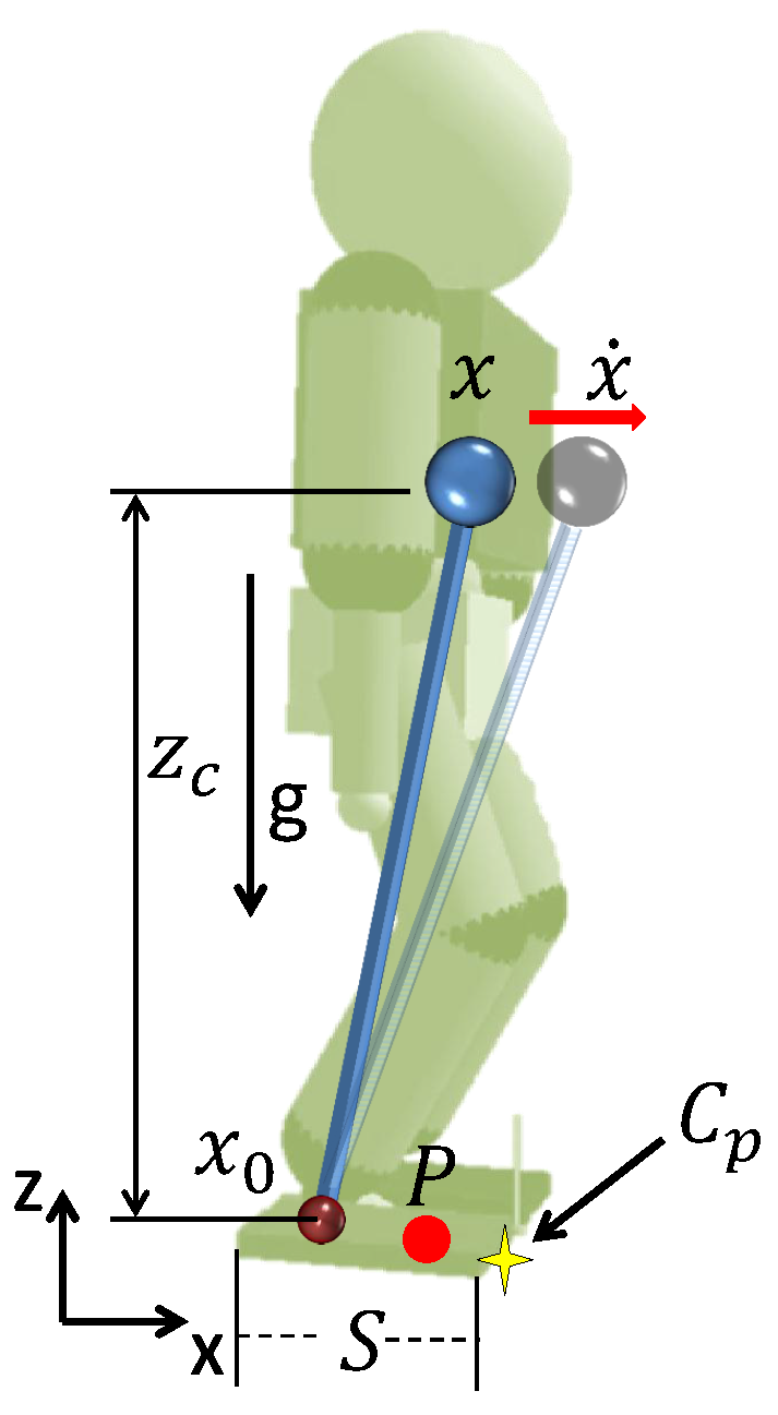
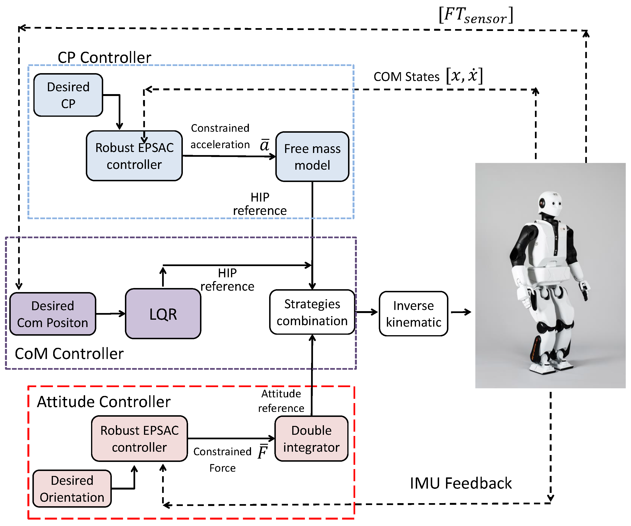
2.1. CoM Stabilizer—A Capture Point Approach

We present the first balance strategy based on the Capture Point Concept [22]. In bipedal locomotion, this concept can be defined as the point C p on the ground were given certain C o M states x , the humanoid’s C o M converges and keeps the Center of pressure P in the given position. The center of pressure P is the point on the support polygon in which the total sum of the contact forces acts. In order to keep static stability, the C o M projection on the ground should be within the support area S; however, for dynamic stability, it holds that
C p = x + x ˙ T c < S ,
where C p is the capture point, S is the humanoid support area, and T c = g z c corresponds to the natural oscillatory frequency of the model. Figure 1 shows the representation of the capture point with z c the height of the C o M .
The aim of this strategy is to absorb the energy due to the external disturbance by applying a hip displacement. With this in mind, we model the C o M using the free body model with mass, f = m x ¨ , which can be represented in state space as:
x ˙ = A x + B u y = C x + D A = 0 1 0 0 B = 0 1 m C = 1 T c D = [ 0 ] ,
where the input to the system is the necessary force that permits the C p to remain in the support polygon while it rejects the external disturbance according to the free-body dynamics. In this strategy, the upper body keeps the upright position and the disturbance is compensated by a compliant displacement at the hip level which absorbs the added energy by the external disturbances.
The feasibility of the method depends on the support polygon limits, which are considered as the output constraints y ̲ and y ¯ into the control loop. In this case, the m i n m a x input constraints are considered to limit the fictitious force that can be applied to the humanoid, and therefore the pass trajectory to the IK is constrained. Additionally, the provided trajectory is limited for the inverse kinematics solver and the low-level controllers of the system, both of them restrict the humanoid dynamics. To implement this balancing strategy, the C o M height in the standing posture, z c , and the mass of the humanoid m are required. The C o M states x , x ˙ are used as feedback.
The final trajectory of the C o M is generated by evaluating the constrained control effort. This describes the desired trajectory of the C o M in the next sampling time so that the C p criterion holds.
Given the simplicity of the model, we can use this strategy in the sagittal and lateral planes using the same control parameters, keeping the non-coupled dynamics and considering just the differences in the support region [16].

2.2. CoM Stabilizer—A Virtual Spring-Damper Approach

Another C o M level stabilizer was proposed based on a virtual spring-damper system introduced to connect the actual C o M position and its reference. By introducing such compliance to the C o M level, the robot was able to cope with disturbances caused by either model discrepancies or unexpected impacts due to early or late foot landing. The generality of the stabilizer’s performance was demonstrated in both standing and walking scenarios on the humanoid robots COMAN [23] and iCub [24].
For a stiff transmission system, at time instant i, the C o M modification, δ r i , that mimics a spring-damper system based on the error between the real and desired ground reaction torque about its axis, τ i real and τ i des , can be calculated in an “admittance” form,
δ r i = δ t k p δ t + k d ( τ i real τ i des z c ) + k d k p δ t + k d δ r i 1 ,
where k p and k d are the desired stiffness and damping of the introduced virtual impedance, δ t is the discrete time step and z c is the C o M height. The details of this stabilization strategy can be found in [17,18].

2.3. Attitude Controller

This balancing strategy compensates the external forces by a natural change of the body’s orientation, mimicking the behavior of a controlled single-degree-of-freedom rotational body [25] that generates a trajectory so that the body motion absorbs the energy through a dissipative motion, instead of acting against the external force. The single-degree-of-freedom rotational motion is described as x ¨ = a , being a the control effort. Therefore, this system does not consider any of the humanoid’s parameters since it is a general representation of rigid bodies. The considered constraint limits the C o M position to the robot’s stability polygon. In this way, both the rotation angle and the C o M position are constrained at each sample time.
During implementation, we take the angular position and velocity measurements or the corresponding states estimator as feedback. These signals are used for the controller, generating the acceleration profile that is applied to the double integrator model. Once the control action is applied to the model, the updated states are used to describe the angular displacement for the next sample time [16].
To make this controller cooperate with the C o M displacement controllers, the C o M displacement generated by the upper body rotation is compensated. This is performed using a three-mass model. In this model, the upper body mass, U B , is composed of the torso, pelvis, two arms, and the head; the lower body mass, L B , is composed of one leg and the other lower body mass F e e t L e g m a s s is located at the foot and comprises the mass of one leg and two feet. Since the feet are mostly stationary during the standing balancing, they do not affect the entire C o M of the robot.
The C o M compensation uses the vector r com = [ x , y , z ] T that defines the deviation of the mass U B with respect to the desired C o M stable position. This value is compensated directly in the overall hip displacement reference. The proposed solution is: Define Δ r as the displacement compensation term to be applied at the hip. This term is computed as:
Δ r = U B U B + L B ( R I ) r com ,
where R is the rotational matrix of the torso, and I is the identity matrix that represents the desired upright orientation of the torso. Notice that I can be changed if the desired orientation is not 0 for the pitch and roll angles.
The displacement Δ r is added to the feedback signal obtained from the C p stabilization strategy. Using this integration strategy the resulting control action at the pelvis does not compensate for the C o M displacement generated by the upper body rotation. Therefore, the precondition of decoupling is guaranteed, and the decoupled controllers can be integrated seamlessly. The balance controller scheme is shown in Figure 2.

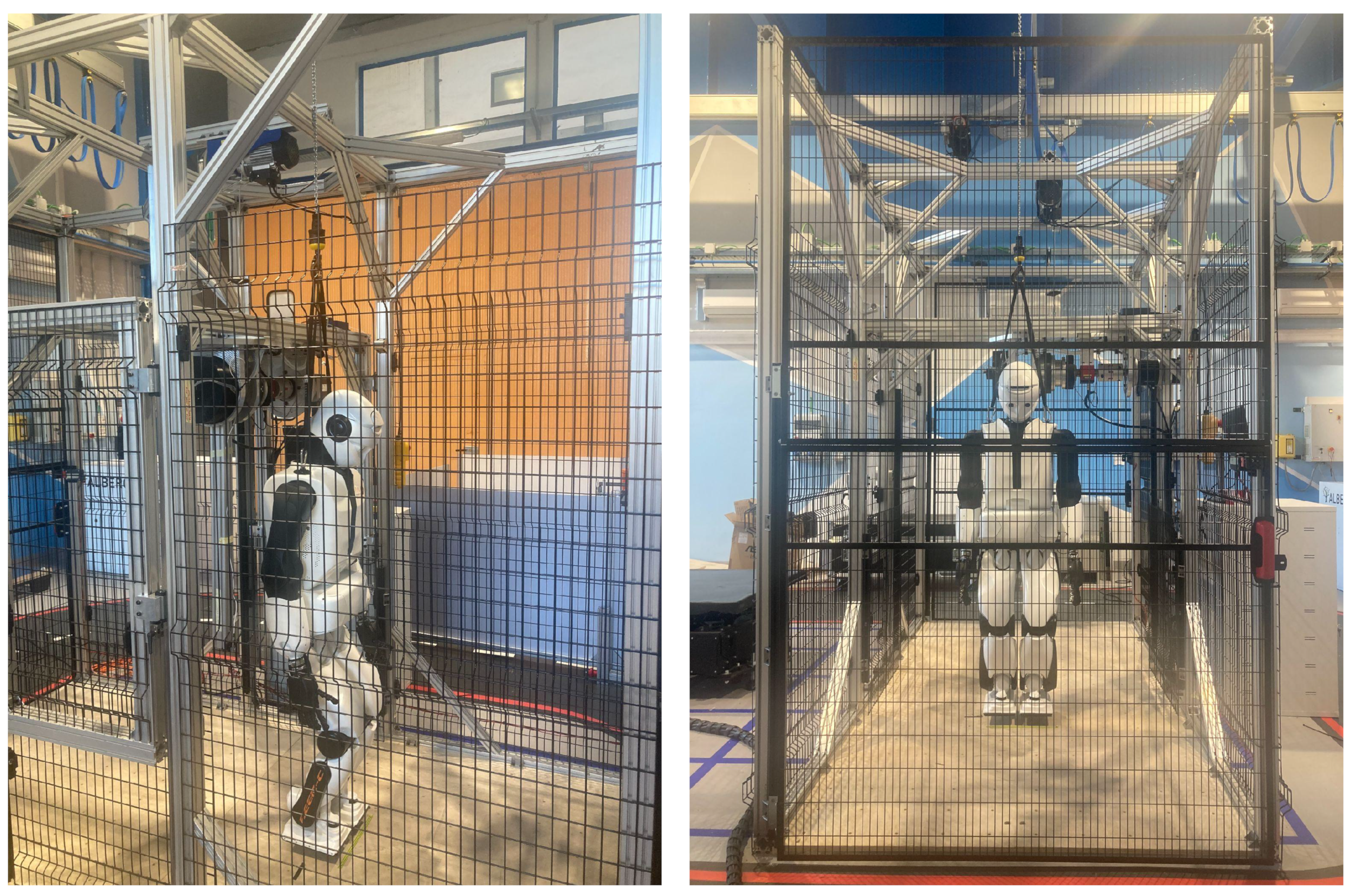
3. Experimental Protocols

To test the performance of the different controllers, we performed a range of extensive experiments at the Humanoids Testing Facility developed by the Italian Institute of Technology under the EUROBENCH EU project [26]. The aim of the Humanoids Testing Facility is to facilitate performance analysis and comparison of different humanoids technologies and algorithms which is a major requirement in our field [27]. For the benchmarking studies carried out in this work, we take advantage of the whole-body control software of the REEM-C together with novel test beds in the facility developed under the COMTEST [28] and DYSTURBANCE [15] FSTPs projects. This was possible thanks to the funding provided to the WALKBENCH project by a second cascade funding initiative sponsored by the EUROBENCH project. For the seek of conciseness, we here report the results related only to the DYSTURBANCE testbed which resulted to be more significant w.r.t. the COMTEST ones.
The DYSTURBANCE testbed consists of a pendulum that can be controlled to generate different types of disturbances with different characteristics. The pendulum height and weight can be adjusted as required and a variety of disturbance protocols are available. A picture of the testbed is shown in Figure 3. To analyze the controllers, in this work we used the pendulum to generate impulsive and sinusoidal disturbances.
To generate the impulsive disturbance, the pendulum started at a defined initial height. Afterward, it performed a free fall, made contact with the robot, and stopped far from the hit position to avoid further interaction between the robot and the pendulum. During these tests, it was possible to set the pendulum height, weight, impact position, and initial angle.
When generating the sinusoidal disturbance, the pendulum moved slowly to establish first contact with the robot. This point was set as the 0 degrees position for the sinusoidal trajectory. Once the pendulum was in contact with the robot, a sinusoidal trajectory was executed with programmable amplitude, along with a set frequency to produce a specific number of cycles. The adjustable parameters were the pendulum’s height and weight, the sinusoidal amplitude in degrees, the frequency, and the number of cycles.
Both protocols were applied in the REEM-C platform, both in simulation and real experiments.
The REEM-C humanoid is a full-size humanoid bipedal robot with 30 DoFs: 7 DoFs per arm, 2 DoFs in the waist, 2 DoFs in the neck, and 6 DoFs per leg. It weighs 80 kg and it is 1.68 m tall (REEM-C parameters were taken from https://pal-robotics.com/wp-content/uploads/2022/01/Datasheet_REEM-C-2022.pdf, visited on 15 October 2022). The REEM-C robot is further detailed in Figure 4.

4. Simulation Results

To prove the versatility of the proposed methodologies and benchmark their performance we first performed dynamic simulations in the GAZEBO simulation environment [29] with the REEM-C model subject to a range of disturbances with different characteristics, as discussed in Section 3. From carrying out these simulations, we are able to analyze the performance of the different controllers considering the C o M deviation, IMU, and Force/Torque measurements. In addition, we compared the performance using the Passive Gait Measure ( P G M ). Refs. [26,27], which defines the capability of optimizing the use of gravity and inertia to move the body forward and can be calculated as:
P G M = 1 R M S ( τ s a ) R M S ( τ t o t ) ,
where R M S is the root mean square, τ s a is the stance feet torque, and τ t o t is the torque at all robot joints.

4.1. Simulations

The different stabilization strategies were tested using the two different external disturbances applied to the back of the robot’s torso. The control used for the first C o M deviation compensation strategy is an LQR with parameters K = 2000 and B = 900 . These parameters were found empirically based on an initial model-based parametrization using the inverted pendulum model.
The model parameters for the C p stabilizer are z c = 70 cm and m = 40 kg considering the mass of the upper body. The controller parameters are: N u = 4 , N 1 = 1 , N 2 = 30 , T s = 5 ms and α = 0.9 . The output constraint was the C p limits which are defined according to the robot’s physical design are Δ x + = 14 cm and Δ x = 8 cm. The optimization problem is solved using Hildreth’s Quadratic Programming Procedure [30]. The output of the system is the C p , however, the signal that reconstructs the desired trajectory is the modeled C o M position. Additionally, for the R-EPSAC implementation, we set the filter observer using a second-order Butterworth high-pass filter with a pass frequency of 5 Hz. Considering that the natural frequency of the robot is g z c = 14.4 rad s , the noise observer provides an estimation of the robot’s natural oscillation effect, but the low-frequency noise is not predicted. It is important to mention that the controller parameters were tuned to provide good performance, but are not optimal.
The body attitude controller does not require any parameter of the robot. Nevertheless, output constraints are considered. In this case, the maximum upper limit is used so that the physical limits of the actuators are not reached, in turn protecting them. The controller parameters are: N u = 7 , N 1 = 1 , N 2 = 10 , T s = 5 ms and α = 0.9 . Again Hildreth’s Quadratic Programming Procedure [30] is used and the filter observer is a second-order Butterworth low-pass filter with a cut-off frequency of 0.7 Hz given the natural oscillation frequency.
Finally, the used C o M deviation of the upper body for the compensator is r com = [ 0 , 0 , 0.2 ] m and the model parameters U B = 40 kg and L B = 10 kg are defined in accordance with the REEM-C size and mass distribution.
For the sake of clarity, in the analysis of the results, we call COM1 the controller described in Section 2.2 and COM2 the controller in Section 2.1.

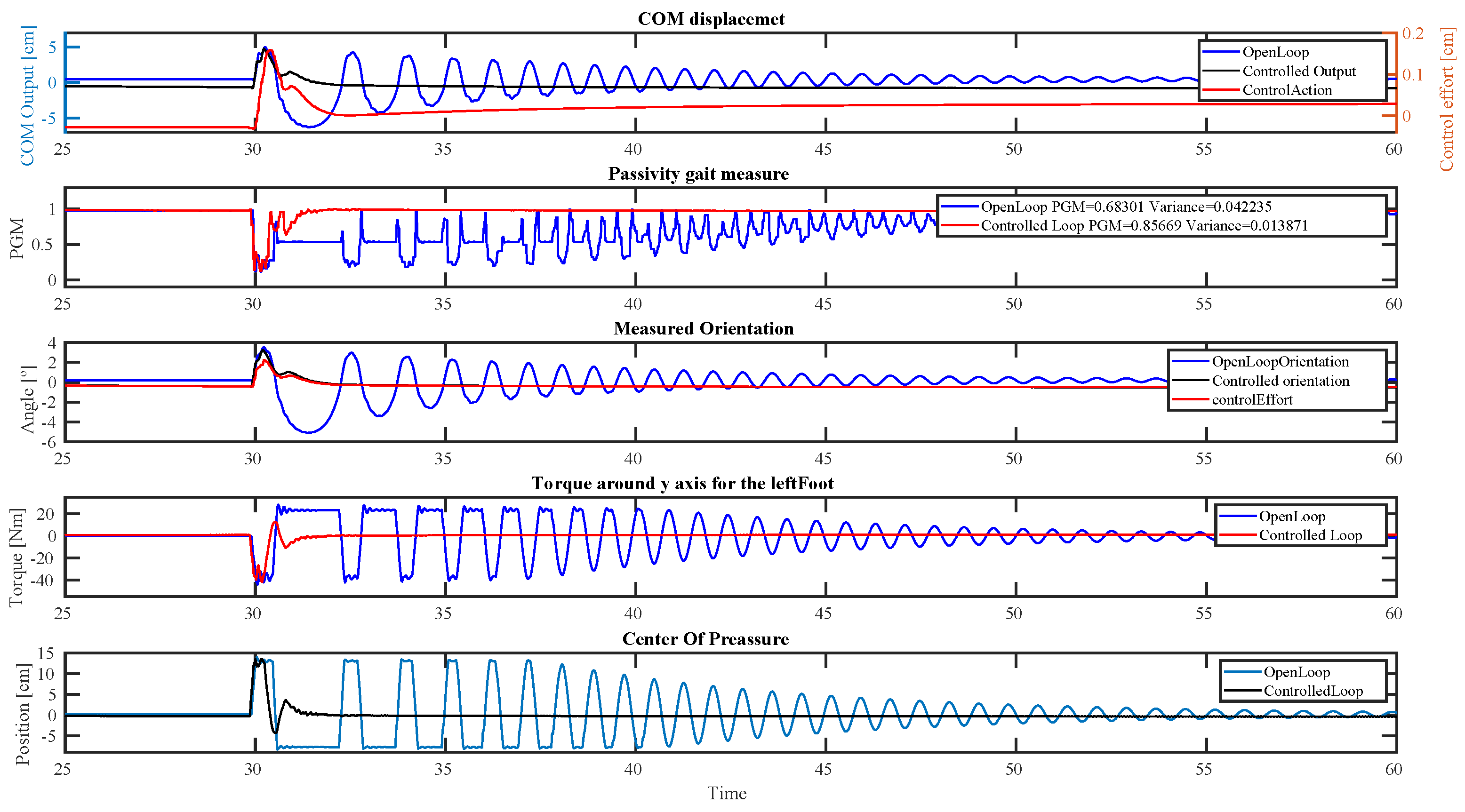
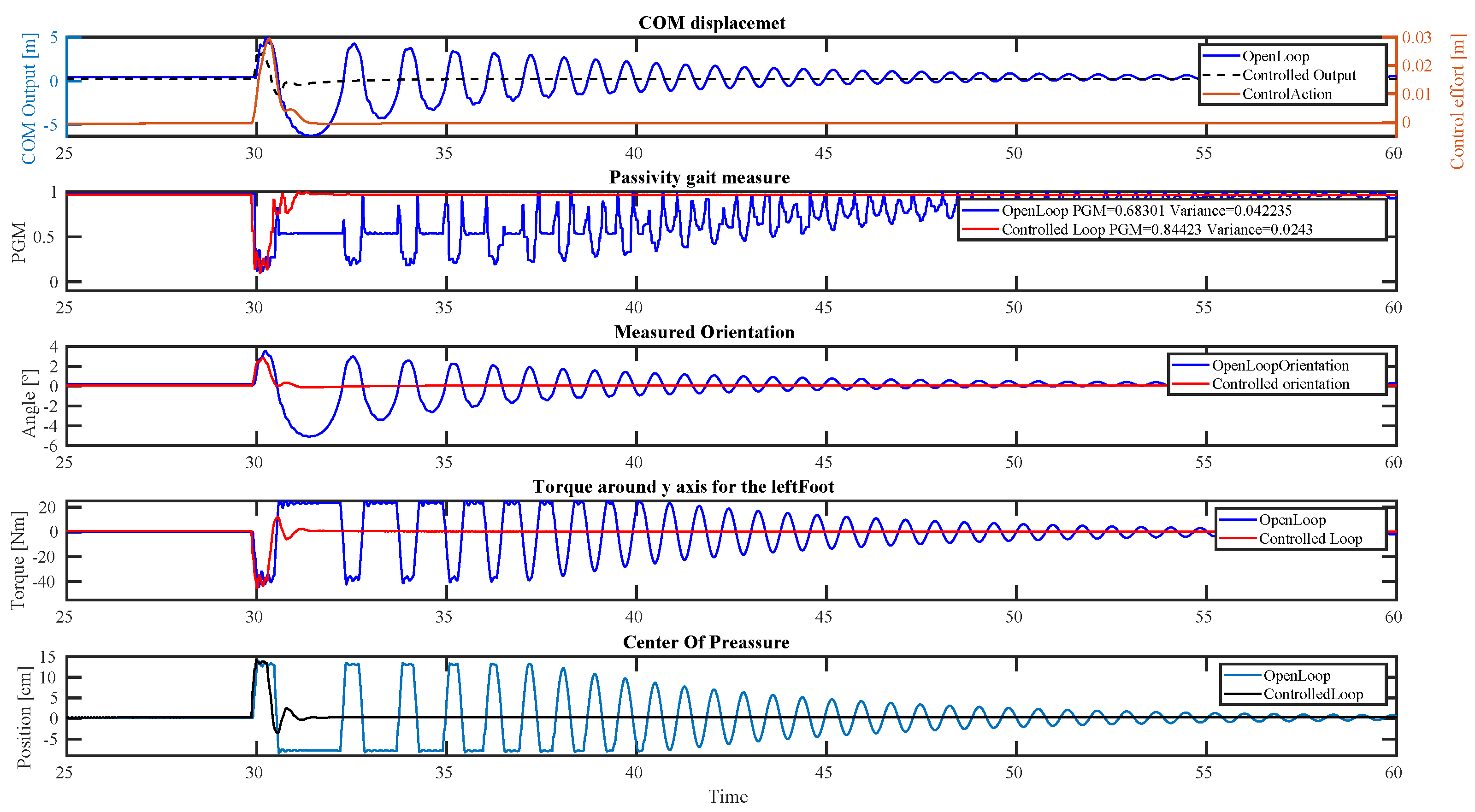
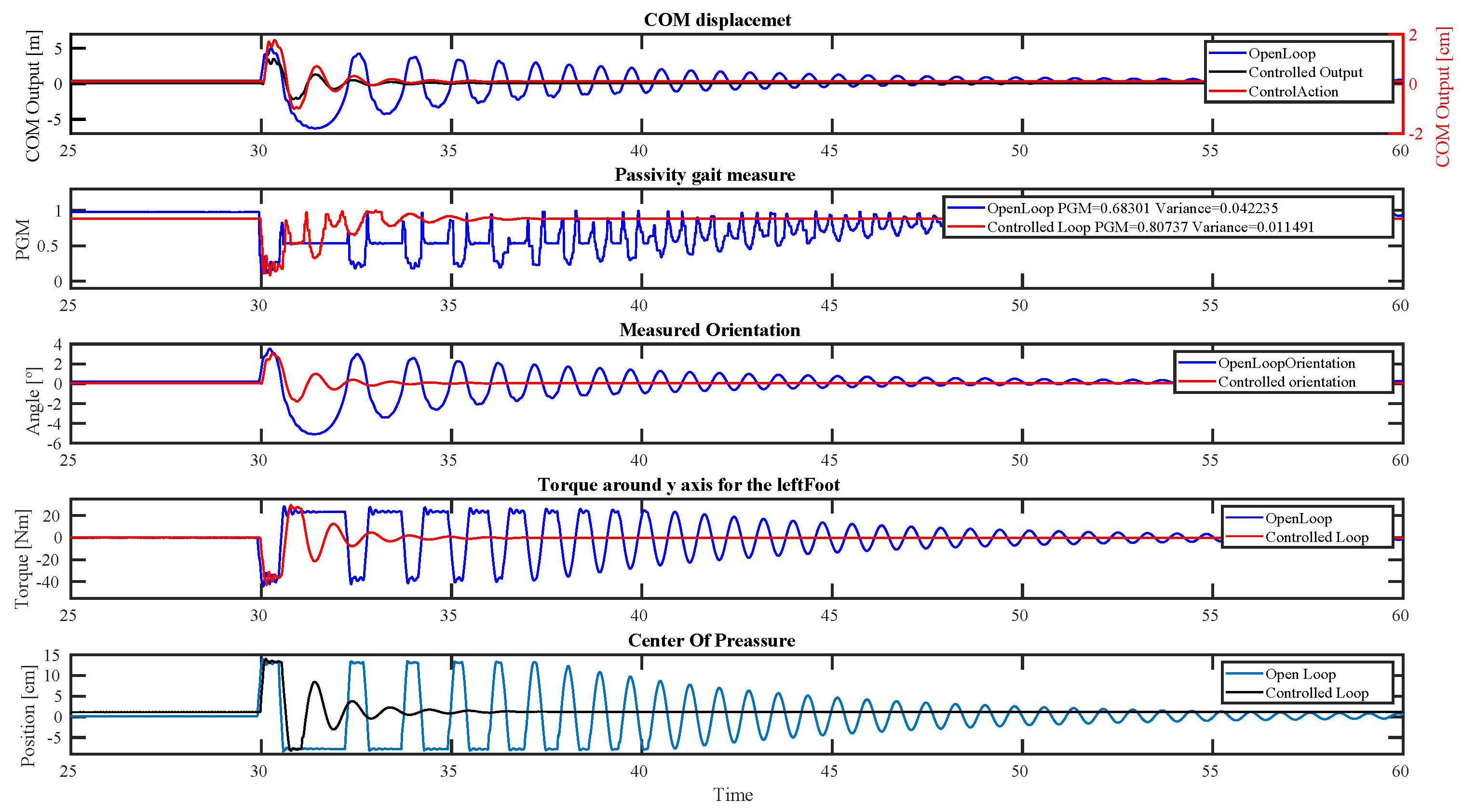
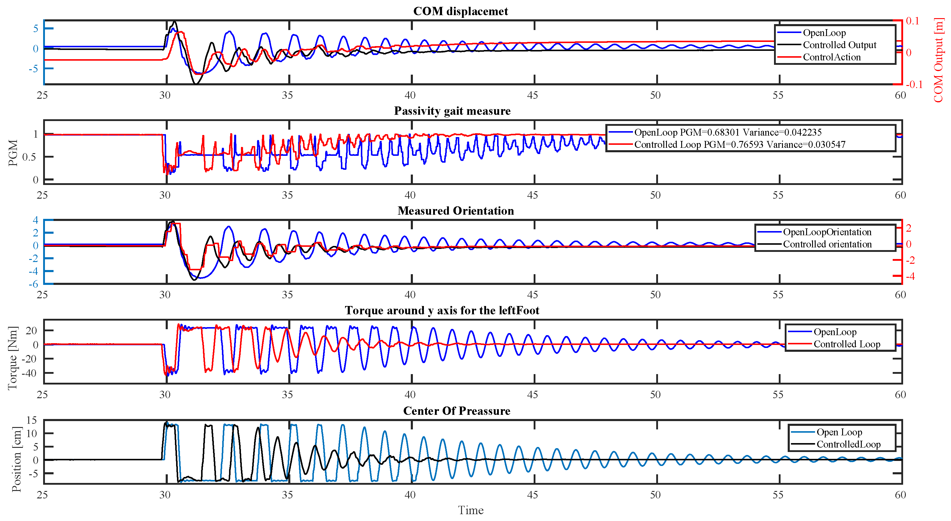
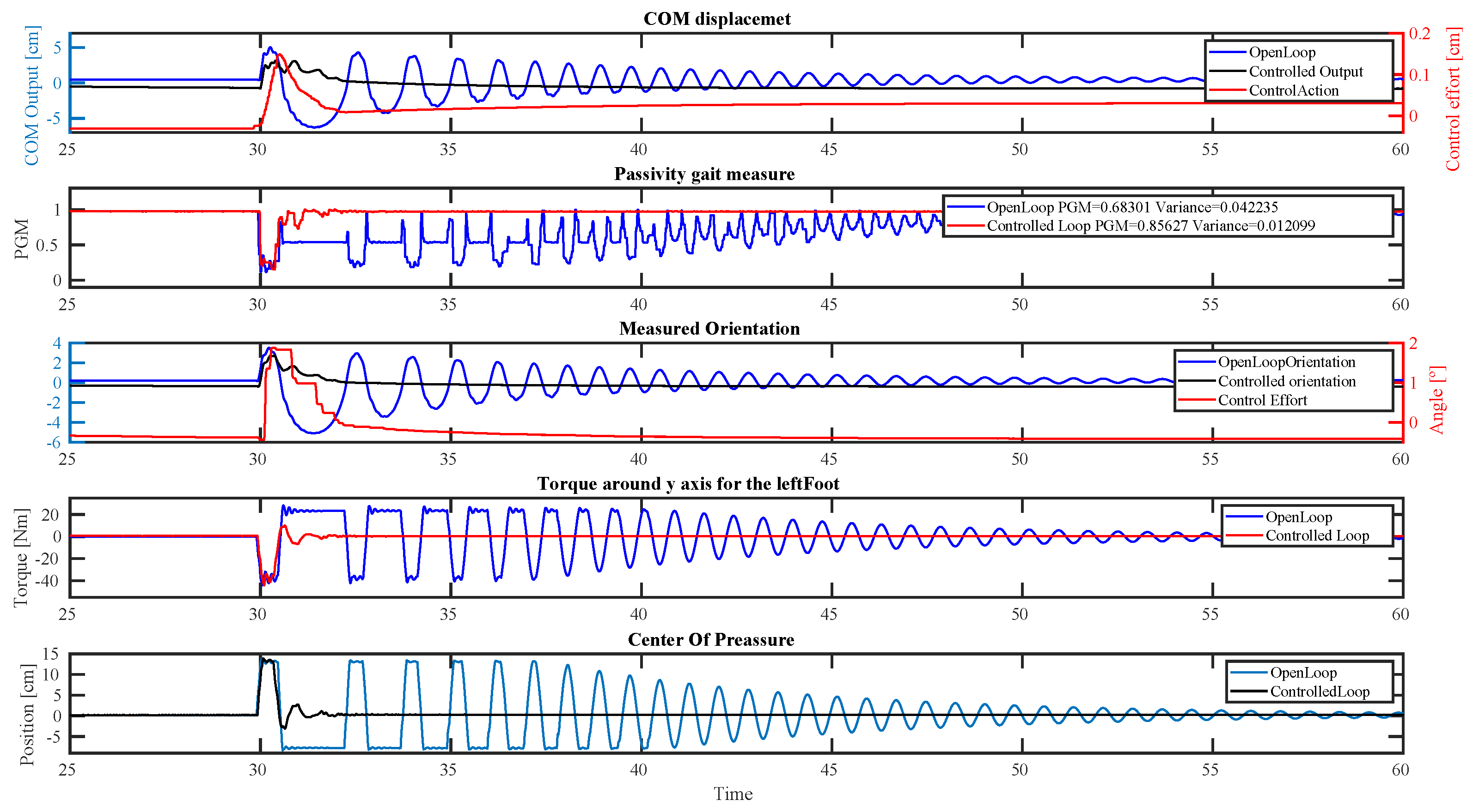
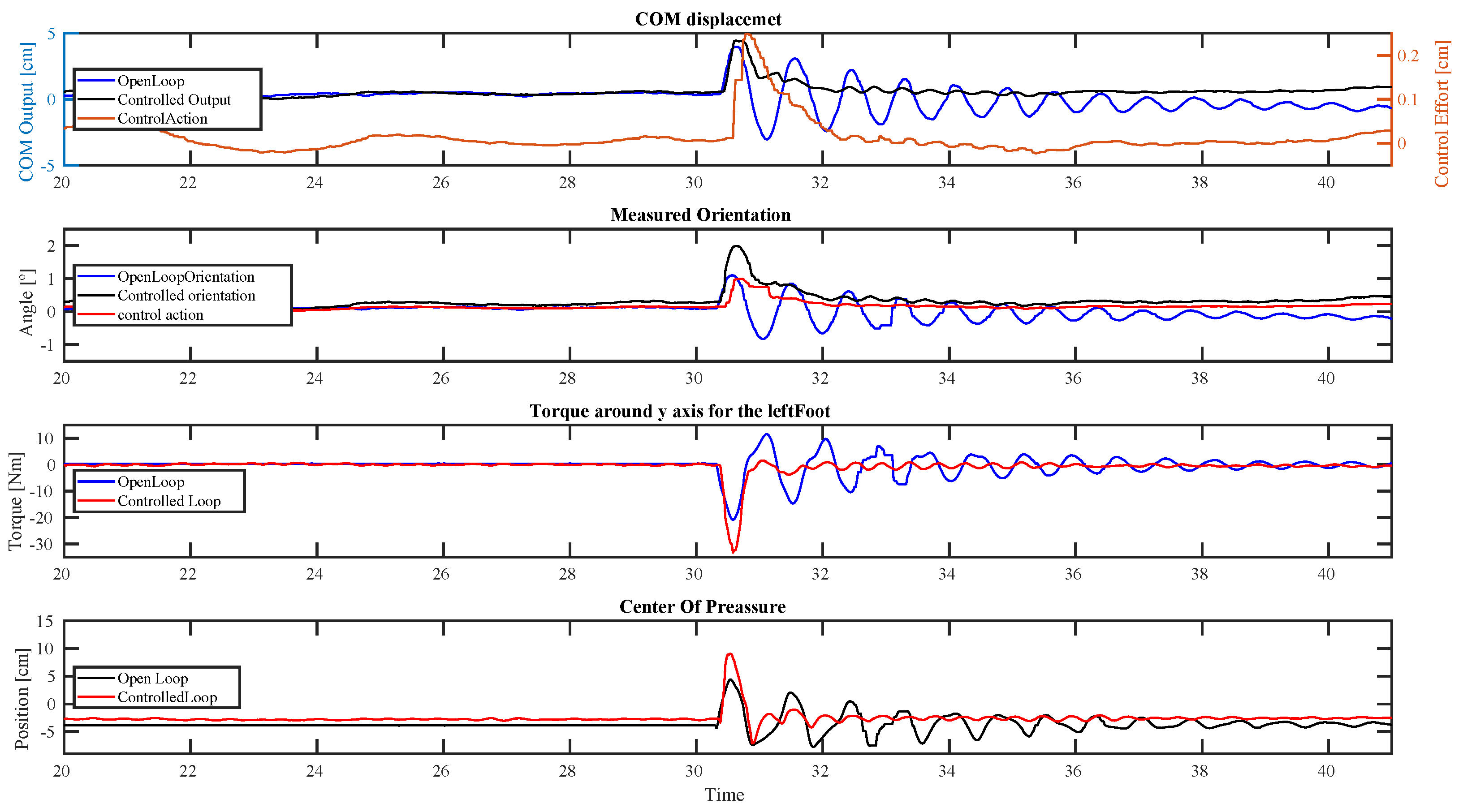
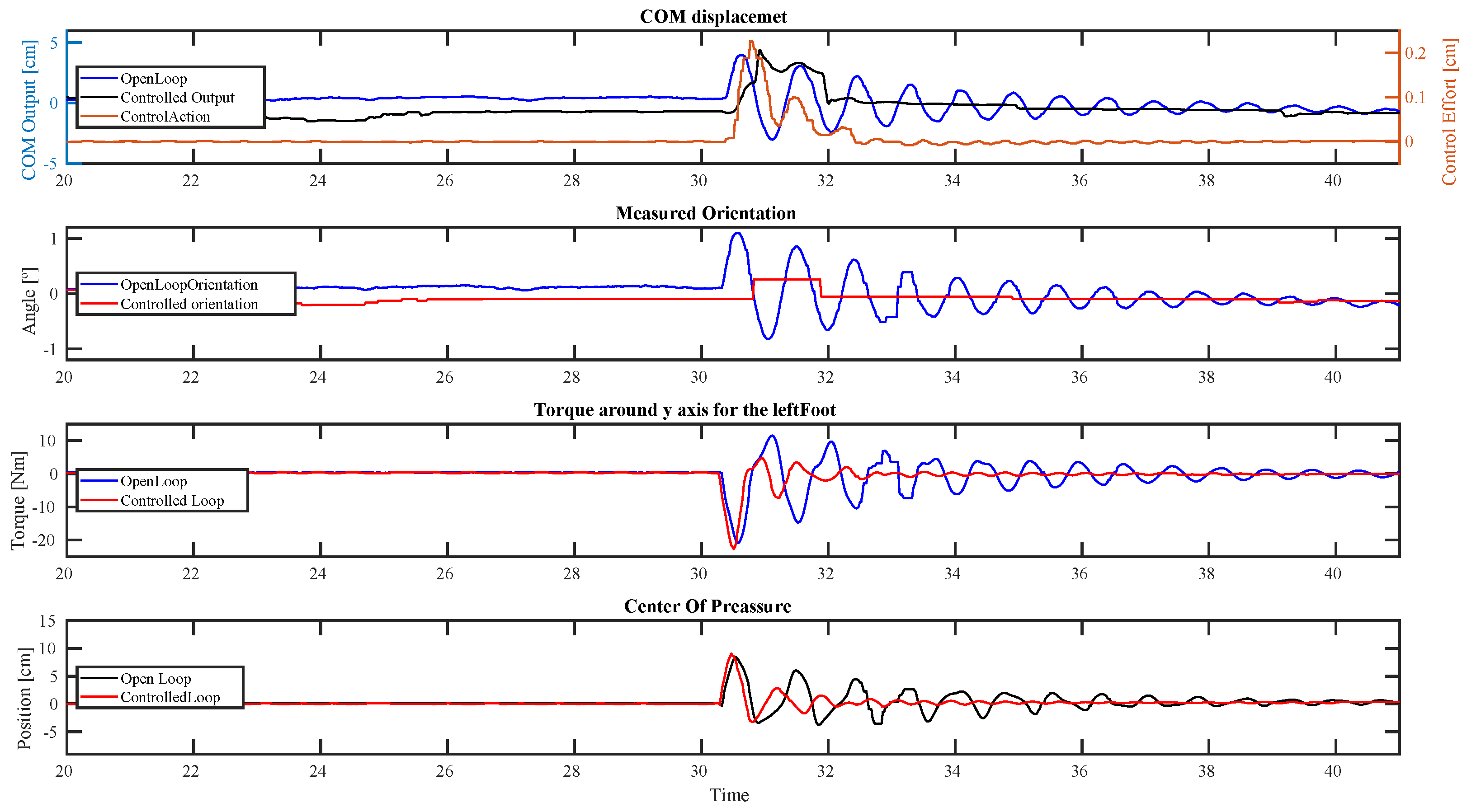
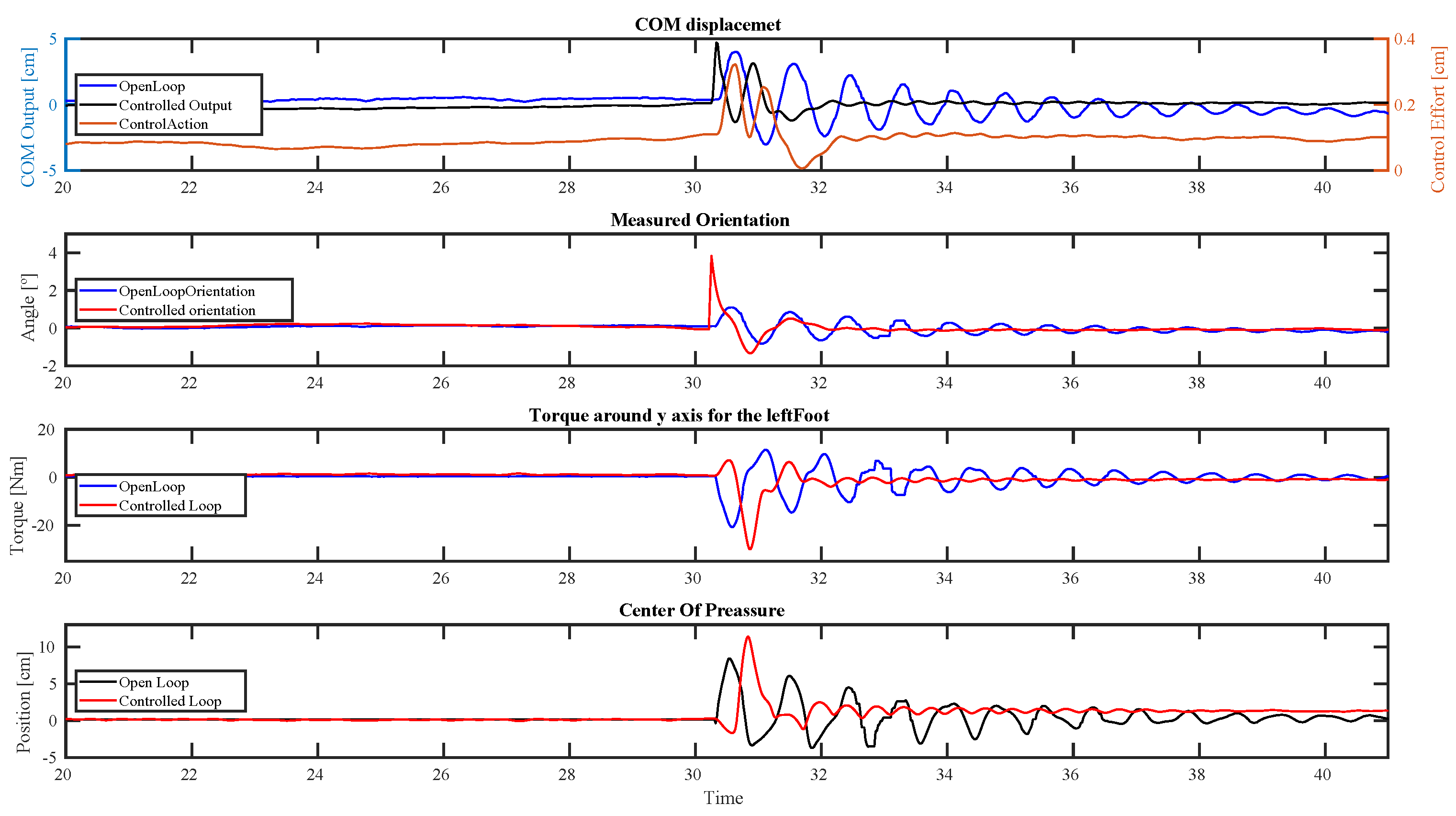
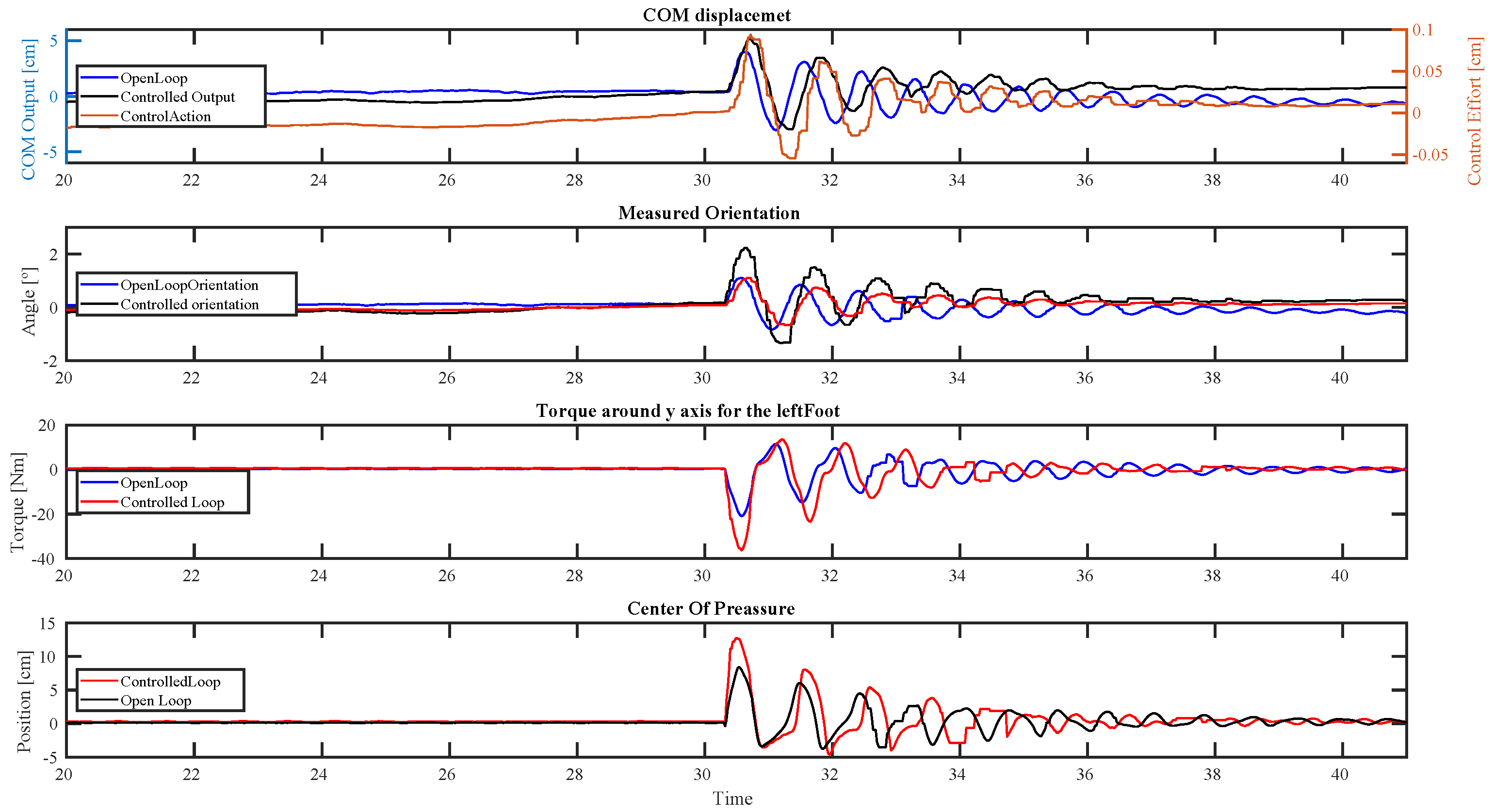
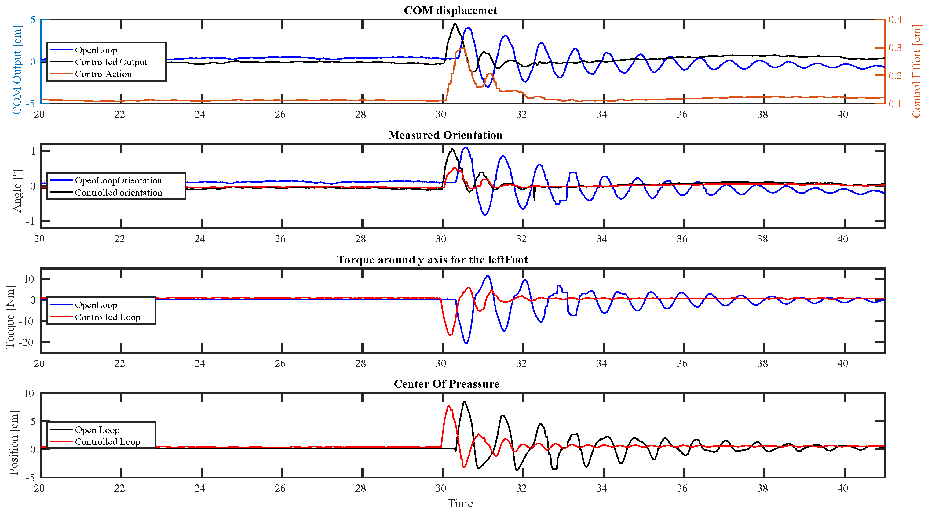
4.2. Impulsive Disturbance

The impulsive disturbance was generated by simulating a pendulum hitting the humanoid with an initial energy of 356 J and an impact force of 235 N. The presented results are compared with the open-loop response of the REEM-C robot with a limited applied impulsive force. We present 5 different figures each one showing 5 plots corresponding to the following controllers:
However, due to the limited space, we only detail the results in Figure 5. Moreover, overall performance conclusions will be given.
Figure 5 reports 5 plots:
  • C o M deviation;
  • Passive Gait Measure;
  • Measured Orientation;
  • Torque around the Y-axis for the left foot;
  • C o P .
In the first plot in Figure 5, we compared the C o M behavior of the open loop response with the response of the controlled case, specifically when using the COM2 stabilizer together with the attitude one. As it is shown, the open loop response takes more than 20 s to stabilize after the impact which is applied at 30 s. It is seen that in both cases, the C o M displacement reaches the same magnitude 5 cm. However, the controlled case stabilizes in 2.5 s. Additionally, the compensation happens in half cycle, implying that the robot did not tilt back as it does in the open loop case. Furthermore, when considering the control action, whose axis is represented on the right-hand side, it is seen that using a small correction of the given C o M leads to a soft, fast, and stable response of the system.
In the second plot of the same figure, Figure 5, we present the calculated P G M (5). As mentioned before, this parameter indicates the part of the effort that the ankle joints do w.r.t the overall robot’s effort. In that sense, a value of 1 means that the effort performed by the ankles to keep the upright posture is smaller than the overall effort, while the closer to 0 the indicator is, the bigger the effort exerted by the ankles is. From the figure, it is seen that the minimum P G M is comparable in both cases but the overall effort is smaller in the controlled one. As detailed in the given legend the RMS is bigger and the variance is smaller which indicates a better performance.
The third plot presented in Figure 5 provides the measured pitch angle. In this plot, it can be observed that the maximum angular deviation is close to 3 degrees without backward oscillations for the controlled case, while there was 6 degrees of backward tilting for the open loop. In addition, the magnitude of control effort, in this case, is comparable to the overall output.
The fourth plot in Figure 5 presents the ankle torque in the Y-axis. In this case, the obtained minimum torque and maximum effort are similar in both simulations. However, the positive cycle of the controller case is already smaller than the open loop one and it happens before the total stabilization of the systems. Therefore, the control action is pushing the robot forward to prevent the robot from tilting backward. This effect can be seen in the first and third plots when there is a slope change in the signals.
Finally, in the last plot of Figure 5, the position of the C o P over time is detailed. In this plot, it can be seen that in the open loop case the robot tilts backward and forwards, reaching the feet limit during the first 8 s. Afterward, it starts converging to the rest C o P position. During the first semi-cycle, the robot keeps the limited position for half a second. On the other side, the controlled loop keeps the maximum tilting position for a shorter time than the open loop did. Therefore, the control action not only stabilizes faster the robot, but it reduces the pressure on the ankle joints as can be also seen in the fourth plot where the torque is reduced w.r.t the open loop case after the first semi-cycle.
Figure 6, Figure 7, Figure 8 and Figure 9 show the performance of the other controllers, respectively, COM1, COM2, Attitude, and COM1 plus Attitude; under the same simulated conditions. Notice that the COM1 and COM2 stabilizers, when used independently, have no control action at the orientation level. Instead, when the Attitude stabilizer is used alone, there is a C o M effort coming from the C o M compensator.
As seen from the different figures. All the control options reduce the stabilization time, although the worst performance is given by the Attitude controller when used independently which has a settling time of 10 s. Under this controller, the robot tilts for several cycles and the C o M moves backward compromising the overall stability. Additionally, even though the COM1 stabilizer compensated for backward tilt when combined with the attitude stabilizer, the stabilization time increased. Instead, by combining the compliant and the attitude stabilizers, the performance significantly increased compared to the single control implementations, as extensively detailed previously.
To carry out a comparison between the proposed strategies, when the robot is subjected to an impulsive disturbance, we collected the results in Table 1. With T s denoting the settling time in seconds after the applied disturbance when the C o M converges to the 90% of the stable position, C o M p stands for the C o M maximum deviation in cm, O r i p is the peak orientation in degrees, P G M the passive gait measure in % and P G M v its variance in %, T ¯ and T ̲ denotes the maximum and minimum torques both in Nm, and finally the maximum and minimum reconstructed capture point C o P ¯ , C o P ̲ in cm. The simulation results show that the mixed control strategies provide better performance in comparison with the single strategies, reducing the settling time and the torques provided by the robot, as reported in Table 1 for the COM1+A and COM2+A controllers. It is also seen that the COM2 controller performs better in terms of P G M variance, however, COM1+A and COM2+A outperform COM2 in all the other KPIs as shown by the bold variables in the table.
Additionally, a bigger stability region is achieved since the C o P remains closer to the initial position w.r.t. the center position. In this case, the P G M indicates the additional effort that the ankle joints apply to provide balance during the gait. An increased P G M means less effort from the ankles w.r.t. the natural posture when executing the whole gait. These results came from the fact that using both strategies together, permits jointly exploiting the upper and lower bodies to compensate for the C o M and momentum variations.

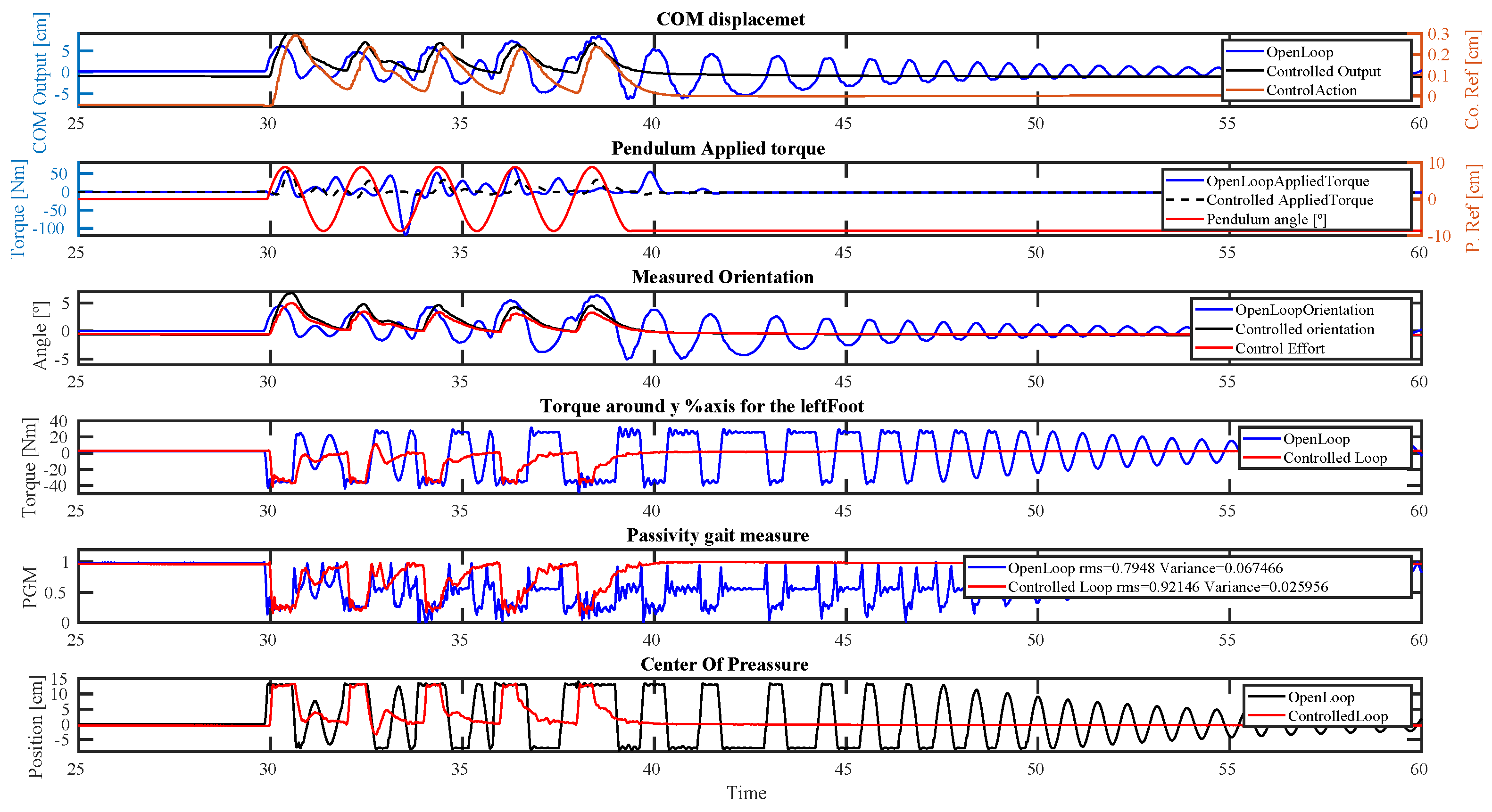
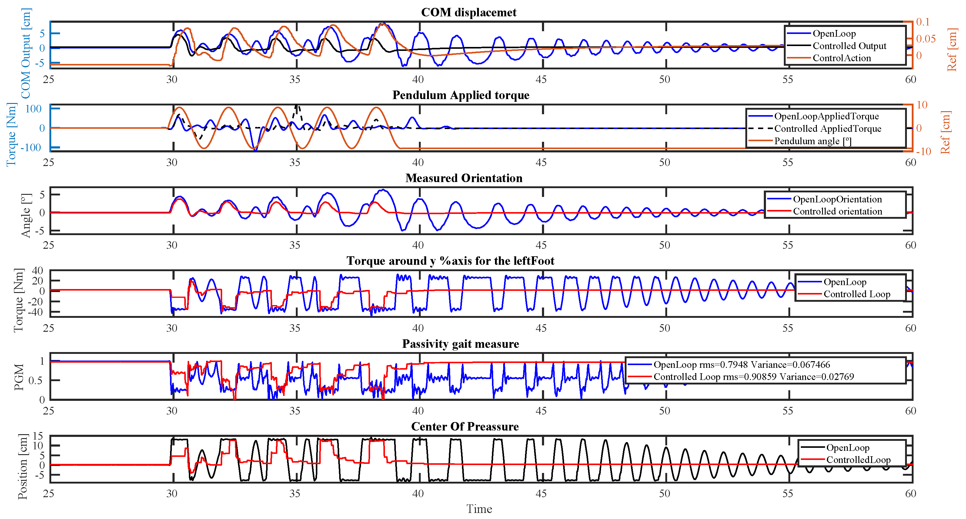
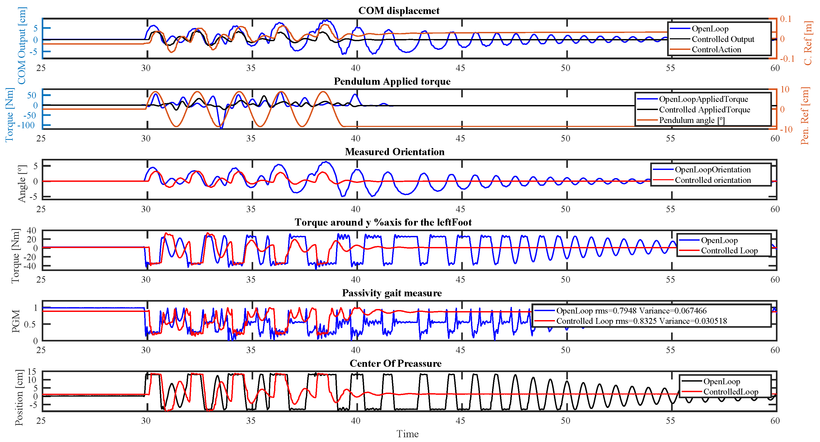
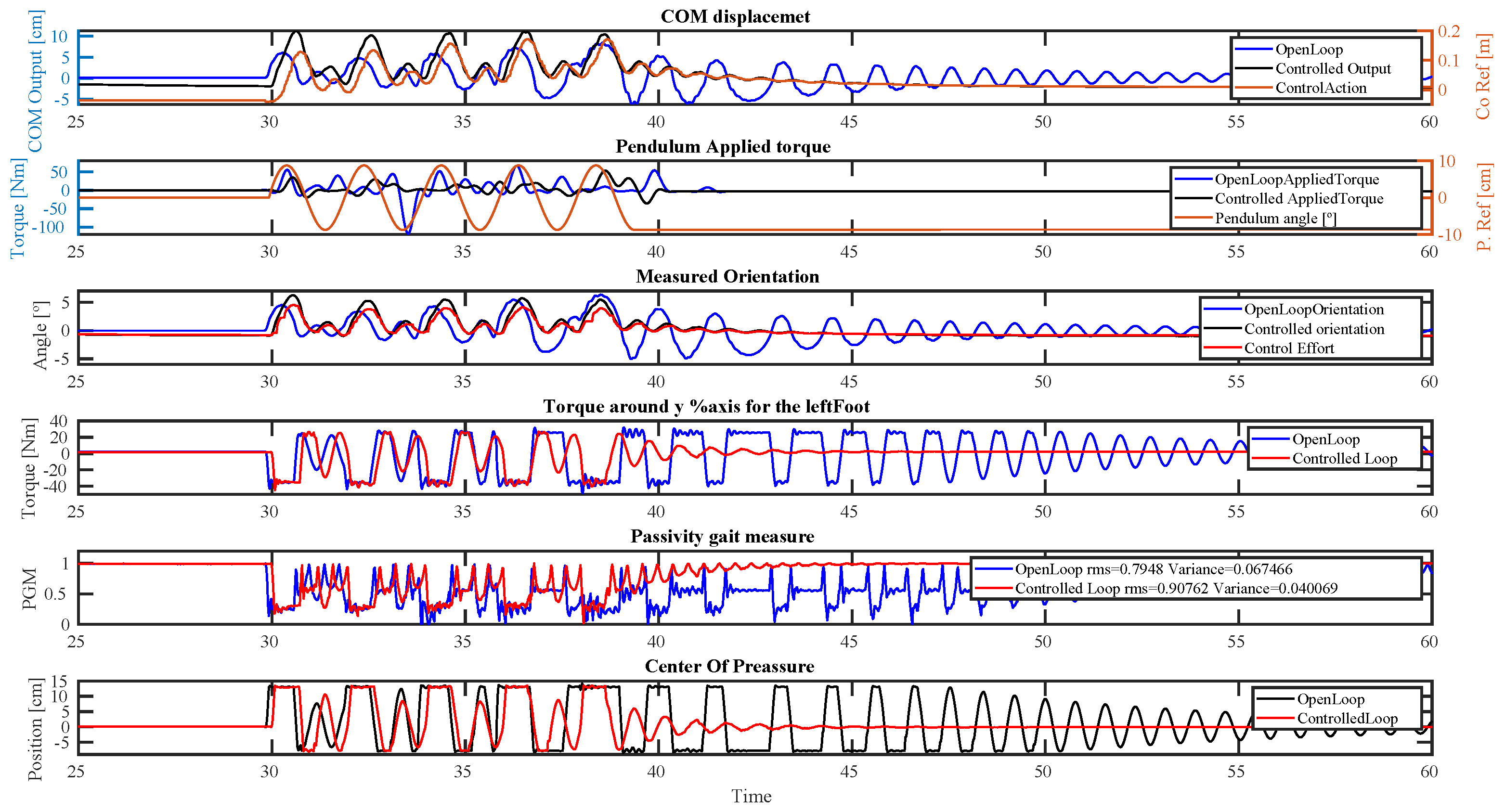
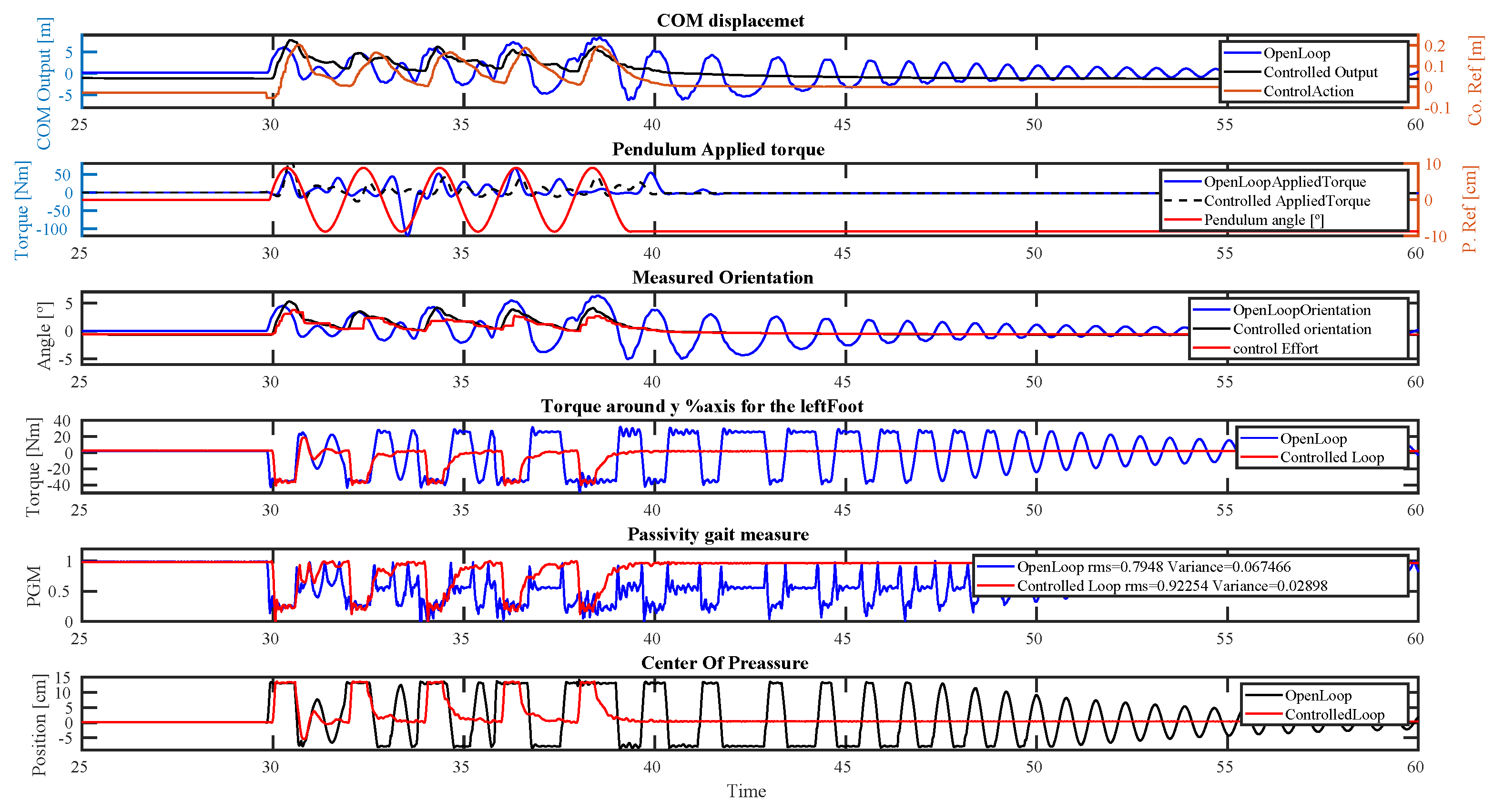
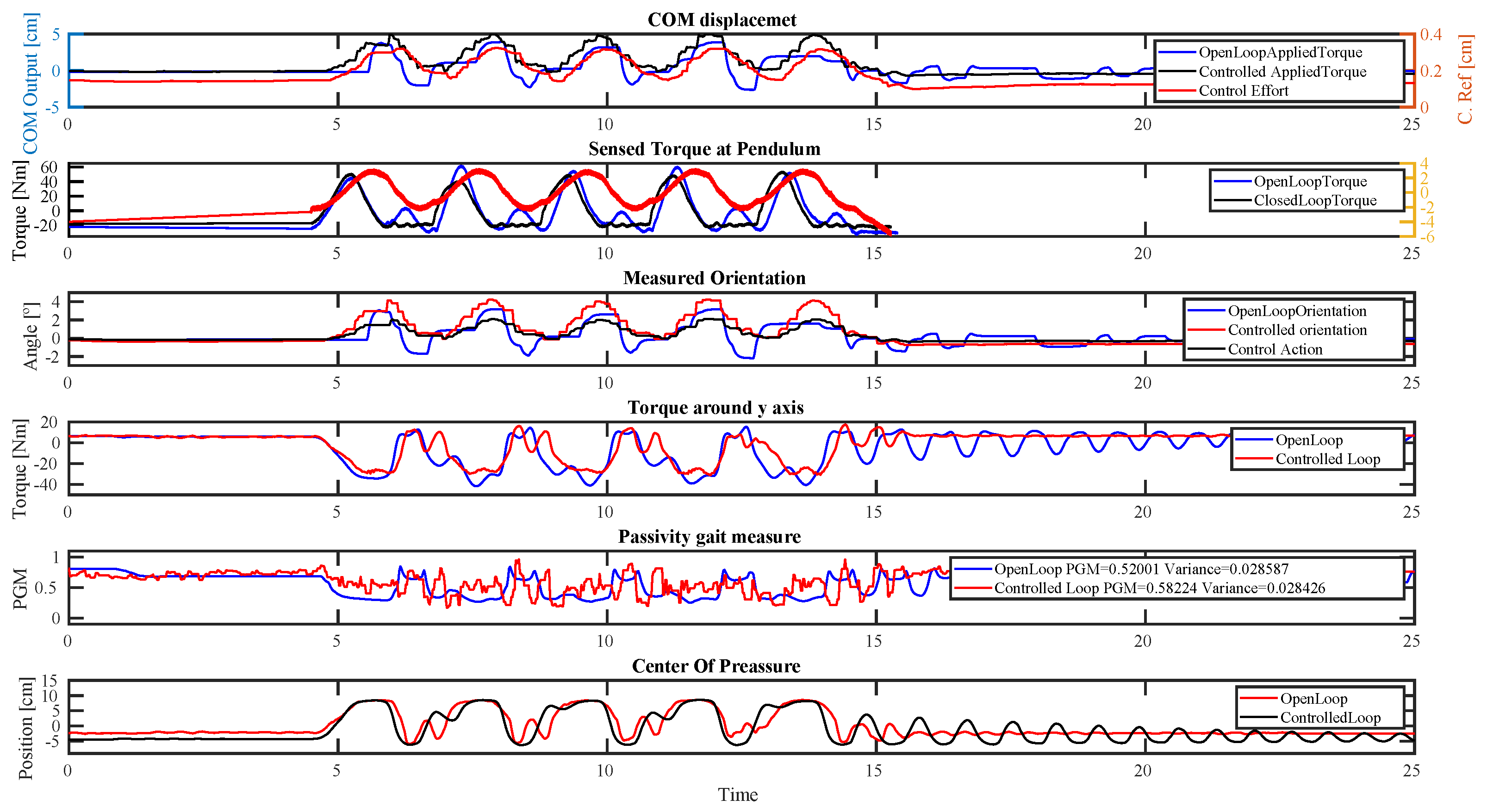
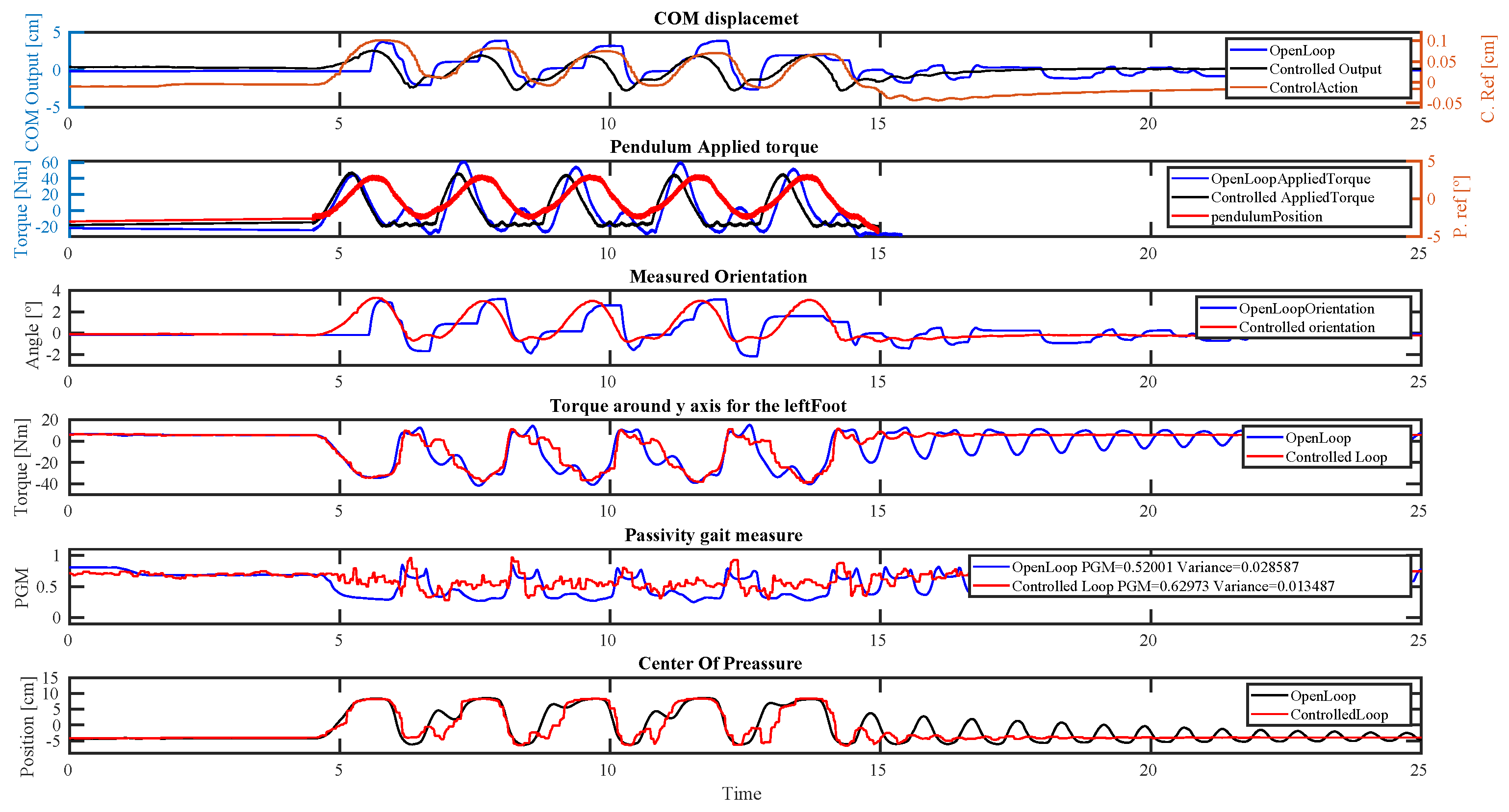
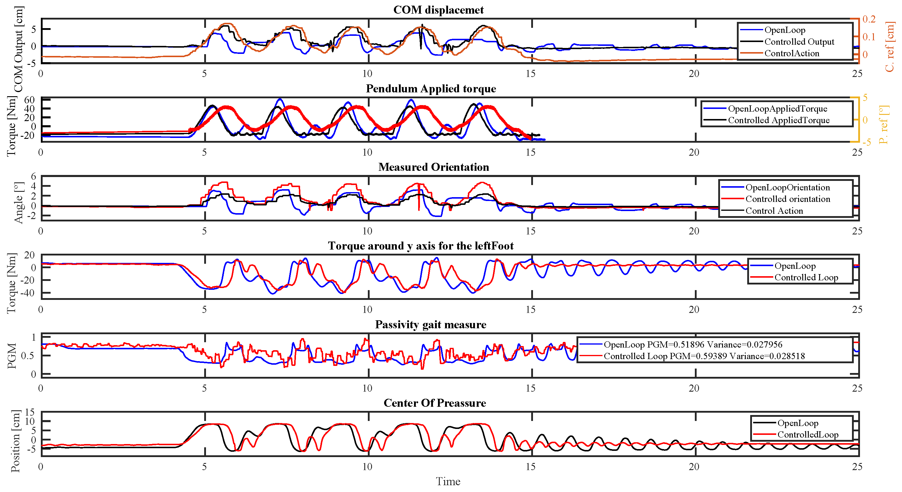
4.3. Periodic Quasi-Static Disturbance

The second set of simulations was run using a sinusoidal disturbance applied by a hanging 50 cm pendulum. The sine wave has a 0.5 Hz frequency and 10 degrees amplitude. That corresponds to 8.6 cm of linear displacement.
As before, we provide an extensive analysis of one case and we present the overall performance conclusions base on the different behaviors.
The 5 figures, each one showing 6 plots corresponds to the following controllers:
As seen in Figure 10, when the sinusoidal disturbance is introduced, the open loop C o M deviation starts moving forward due to the pendulum action, on the upper plot, the tilting back is compensated by a short period, but at a certain moment, the pendulum loses contact with the robot. At that point, the robot starts a short back/front oscillation that is stopped by the pendulum during the second cycle. When the third pushing cycle starts, the pendulum regains contact with the robot when it was already moving forward, as a result, the C o M deviation increases with regard to previous cases and it does the same for the fifth cycle. This happens given the proximity of the selected sinusoidal frequency and the natural robot’s frequency. After the last cycle, the robot tilts back 5 cm and afterward, it converges to the rest position in more than 20 s. When analyzing the controlled response, the COM2 strategy together with the attitude stabilizers causes the C o M deviation to be bigger w.r.t the open loop case, however, the back tilting effect is compensated after losing contact with the robot. Therefore, there is no resonating effect, as we saw in the open loop case. Instead, it is worth noticing that the displacement in the first cycle is bigger than in the following cases. This is due to the fact that during the first cycle the robot is in a stable position and the control action is small if existing, therefore, when the first disturbance is applied, the compliant motion at the C o M of the robot absorbs the pendulum sinusoidal action by moving in the forward direction. Instead, in the following cycles, the robot is under a controlled action moving the robot backward and stabilizing the desired resting position. Therefore, when the new disturbance takes place, there is already a control action overcoming the new applied disturbance. After the last cycle, the robot converges smoothly to the stable position without tilting back. The control action is in agreement with the C o M motion and its magnitude agrees with the one analyzed in the previous disturbance scenario.
The second plot shows the effort that the pendulum exerts when applying the disturbance. The open loop case shows how the pendulum supports the robot when tilting, therefore, the pendulum applies additional effort to prevent the robot from falling faster. This is reflected in the positive torque during the negative semi-cycle of the pendulum whose position is reflected on the right axis. Afterward, the pendulum effort decreases once again, since the robot tilts forwards. Later it increases again and the pendulum applies the next cyclic disturbance. As can be seen, the pendulum effort is smaller in the controlled case and stabilizes at zero immediately after the last cycle. In the open loop case, there is an additional bump, showing the interaction of the robot with the pendulum in the static position.
The motion of the robot can be better analyzed in the third figure. As it is seen, the orientation performance in the open loop case. tries to tilt back twice after each cycle and the first tilting, in particular, increases on each cycle reaching 5 degrees in the fourth cycle. This behavior does not appear in the controlled loop as previously stated.
In the torque analysis, the fourth plot of the figure, it can be seen that the open loop torque has a different performance on each cycle. As said before, this happens due to the difference between the natural oscillation frequency and the applied disturbance one. In the first cycle, from 30 to 32 s, the robot reaches the maximum torque when moving forward and later it oscillates backward, forward, and backward again, without saturating the torque, before the new disturbance cycle starts. During the second and third cycles, from 32 to 34 s and from 34 to 36 s, respectively, the backward oscillation is bigger and saturates the applied torque for a longer time as can be seen at 34 s where we have a negative saturated torque and at 35 s with a positive saturated one. Finally, the last cycle enters into action when the robot is tilting forward and the maximum torque is already being applied. This can be seen between 37 s and 39 s where the open loop torque response is saturated for the longest period. When we look at the controlled case, we see that the applied torque pulls back the robot in 4 of the 5 disturbances, only in the second cycle, from 32 to 34 s, there it is required to apply a positive torque to prevent the robot from tilting back further as can be analyzed from the positive torque occurring at 32.5 s.
The P G M , in the fifth plot, shows a coherent performance with the previous analysis with a smaller variance and a better P G M measure from the controlled case w.r.t the open-loop case. Finally, the C o P moves forward to the limit in both cases but never backward in the controlled case. Notice that the time the C o P stays in the limit position reduces over cycles in the controlled case, while it increases for the open loop scenario.
From these simulations, we can remark that the COM1 stabilizer has some back tilting during the first cycle while the displacement is smaller for all the disturbances. Notice as well that the center of pressure moves forward for a longer period over time. The COM2 controller has a bigger C o M displacement in both directions and so does the orientation. By looking at the P G M we see that the best performance is reached when using the combined strategies, increasing it by 2 % for the COM1 case and 10 % for the COM2 case. This means that the overall effort during the simulation is reduced in that percentage.
Table 2 collects the data for comparison purposes. In this case, T s refers to the settling time from the first pendulum contact with the robot to its stabilization. We took this time considering that the contact with the pendulum after the last sinusoidal cycle is not consistent throughout the different studied cases. The other values stand as previously named. In this case, we can see that the combined stabilizer provides a better P G M factor while reducing the positive torque applied by the ankles (tilting backward), with an additional reduction of the C o P displacement. Instead, the negative torque is comparable with the open-loop case and can not be further compensated since the robot is being pushed forward by the pendulum. Consequently, the C o P displacement can not be compensated. It is worth noticing the orientation behavior in simulation. As shown in Table 2, when using only the COM1 and COM2 strategies, the change in orientation is smaller with regard to the other cases, instead, when applying the attitude stabilizer as a single or additional strategy, a compliant reaction at the torso is added to the compensation motion.
The highlighted variables in Table 2 indicate the best controller performance for the respected KPI, as can bee seen the COM1+A and COM2+A strategies have an outstanding performance in the KPIs that are not saturated by the disturbance while keeping a comparable performance in the remaining KPIs. Notice that the C o M p and O r i p are bigger in this case for the two balancing strategies due to the compliant behaviors as previously mentioned.
In the following link is possible to find videos of the performed simulations and experiments https://youtu.be/F7ATTcEGi9U visited on 15 October 2022.

5. Experimental Results

The same protocol presented in the simulation was consecutively tested in the real platform.
The COM2 stabilizer was using the same gains we used in simulation while for the COM1 we changed the LQR gains to K = 1200 and B = 400 for the real experiments. The rest of the parameters were kept the same.

5.1. Impulsive Disturbance

To run this protocol, we used a 1 m pendulum weighting 3 kg. The pendulum was driven to a 90 degree position and left in free fall. After the pendulum hits the robot, it moves back to prevent further robot-pendulum interaction. The pendulum was set to hit the robot on the back. From the setup point of view, it was necessary to hit the robot in a lower position with regard to the simulation scenario, to avoid damaging the electronics and accidentally pressing the emergency stop located at the back of the robot. In addition, we use a soft cover to protect the robot. Therefore, some additional damping was given to the robot’s original structure. Results are presented using a similar structure as the one used for the simulation scenario. The fourth plots presented on each figure, corresponding to each control case, are: C o M deviation, Measured orientation, Torque at the left ankle, and reconstructed Center of pressure. As before, we will comment on one figure and leave the following ones to the reader. However, a general conclusion will be given.
In the first plot in Figure 15, it can be seen that the open loop response presents more than 20 s of oscillations after the impact. This agrees with the simulated results. In addition, we can see that the maximum displacement is ≈4.5 cm. When we compared this performance with the controlled case, COM2 with Attitude stabilizer, we see that the controller is able to stabilize the disturbance in 2 s without any back tilt. The response shows that the robot moves back fast and, before reaching the initial position, the response decelerates so that it converges slower and softer. Finally, it is worth noticing that the control effort agrees with the C o M motion and the magnitude is close to the values given in the simulation part. This is one order of magnitude less.
When looking at the second plot, which shows the measured orientation, the presented figures are quite similar to the C o M response in the first plot. As can be seen, the control action reflects with a smaller magnitude the initial half cycle of the response, when the robot is recovering the initial position, the orientation reference keeps the reference forward, therefore, decelerating the C o M response.
The third plot shows the effort made by the ankle joint during the experiment. As can be seen, the open loop response has a lower effort but it oscillates and lasts longer. The controlled case, presents a bigger effort, moving back the robot and allowing its stabilization. We can see that the torque becomes positive when the control effort for the orientation stays constant and the C o M displacement in the first plot changes the slope from negative to positive, this happens around 31 s, this is one second after the disturbance is introduced. This shows that the control action is pushing forward the robot before it reaches the initial position.
Finally, in the last plot of Figure 15, it is possible to see that the C o P moves up to 10 cm, which is further that the open loop case. We can compare this response with an ankle-like response, therefore, pressing with the toes to push back the robot, and then compensating for the overcompensation by pressing forward with the ankles.
Looking at the results presented in Figure 16, Figure 17, Figure 18 and Figure 19 corresponding to control scenarios COM1, COM2, Attitude, COM1 with Attitude, and COM2 with attitude, respectively, we see that both COM1 and COM2 stabilizers are able to stabilize the robot in the first 2 s. When using the attitude stabilizer, there are oscillations during 9 s which is not desired but in general better than the open loop response. When implementing the cooperative cases, COM1 (COM2) with Attitude controller, the stabilization time does not improve but the response is softer in both cases and more continuous. As seen in Figure 19, first plot, the COM1 plus attitude controller tilts back for a small portion at 30.5 s which was not present in the COM1 response in Figure 16.
For the first set of experiments, we collected the data in Table 3. In this case, the P G M was not measured but the rest of the metrics are given as in the simulation results due to bandwidth issues during the experimental phase. As can be seen, the results are consistent with the simulated ones. The combined strategies were able to reduce the applied torque at the ankles in both recovery phases and provide faster stabilization times. Given the compliant behavior of the controllers, it seems that the C o P was negatively affected since the motion ratio is bigger in comparison with the open loop case. The best KPI for each case is highlighted in the table.

5.2. Quasi-Static Periodic Disturbance

For this set of experiments, we present three cases which are: the COM1 controller, which has shown in all the previous results the best performance over the single control implementations. The other two experimental cases we present are the cooperative case of the COM1 with the Attitude Stabilizer and the cooperative case of the COM2 with the attitude stabilizer as well.
On each of the experimental results shown in Figure 20, Figure 21 and Figure 22, we present six different plots as we did in the corresponding simulation scenario.
Comparing the C o M deviation is possible to notice that the three different control cases stabilize the C o M after each interaction with the pendulum. However, the COM1 case, in Figure 21 has a small back-tilt, which does not appear in the other cases. In the first plots in Figure 20 and Figure 22 is shown that the C o M of the robot moves forward but does not tilt back. This behavior can be observed as well in the second plot for each of the figures which correspond to the sensed torque by the pendulum. As can be observed, for the open loop case, there is an interaction of the robot with the pendulum when it is moving forward. Therefore, when the robot is tilting back, the pendulum is decelerating the robot and a positive torque appears in the measure. When looking at the same plot for the closed loop cases, we see that after the positive cycle of the sinusoidal, the torque remains negative, moving back to the pendulum without any robot-pendulum interaction.
The third plot, measured orientation, shows similar behavior for the different control scenarios, while the open loop case keeps oscillating slightly for the remaining time of the experiment. The time response of the controllers and the open loop cases is better seen in plots 4 and 6 on each of the studied figures, where for the open loop scenario, the ankle torque, and the C o P keep oscillating during the remaining time in the figure. This is from time 15 s when the applied disturbance stopped, to the end of the plot at time 25 s. Therefore the robot is tilting back and forward at the natural robot’s frequency. This behavior does not appear in the controlled cases, where the ankle torque and the C o P stabilized around 17 s, This means, 2 s after the disturbance had finished.
The data from the final set of experiments have been collected in Table 4. Despite the behavior of the three considered balancing strategies being quite comparable, the COM1 performs better. The only measured KPI where the combined strategy COM2+Attitude performs better is during the recovery phases, providing a smaller torque w.r.t the other scenarios. Interestingly, in comparison with the simulation results, the orientation of the robot is not affected as expected. However, it is seen how the compliant performance of the C o M provides a bigger horizontal motion of the robot to dissipate the applied disturbance when using the combined control strategies. Looking at the P G M , the best performance is given by the COM1 controller which increases the P G M ’s RMS by 11 % while the combined control performance increases it by 8 / 9 % . Moreover, the variance in COM1 is reduced by half, while the other cases remain in the same range. (It is necessary to remark that collected data are not as clean as desired and might affect the given results). The best KPIs obtained during the experiment for the different controllers are highlighted in Table 4.
As previously mentioned, in the following link is possible to find videos of the performed simulations and experiments https://youtu.be/F7ATTcEGi9U visited on 15 October 2022.

6. Conclusions

In this paper, we evaluated the performance using standardized protocols of three different balancing strategies that can be integrated to provide balancing capabilities for humanoids. The single strategies presented good balancing performances with the capability to reject external disturbances with compliant and soft responses. A further performance increase was shown when the strategies are properly integrated, generating cooperative behavior. This was performed using a compensation strategy that considers the C o M deviation due to the control action of the attitude controller, upper body rotation. Therefore, by considering the C o M interaction of the different agents that acts over the controlled C o M variable, a natural cooperative scheme emerges.
The simplified models used in the balancing strategies, the double integrator, mass spring damper, and the free body with single mass models, permit to easily port the proposed approach to different bipedal robots requiring quantities, such as the mass and the C o M height, which are usually available and well known in humanoid robotics. Furthermore, the only required feedback signals are provided by the IMU, Force/Torque sensors mounted at the feet, and from the C o M states estimation. Moreover, by integrating the proposed methodologies, natural and compliant response with an ankle or a hip strategy is achieved without the need of switching control strategies.
The different balance strategies were tested in standardized testing beds. This allows for repeatability of the experiments and simulations by other researchers, and comparison of the obtained results with other balancing strategies. The obtained data represent a valuable tool for the selection of different balancing strategies.
To extend the present results, it is necessary to benchmark the given balancing strategies under a wider set of scenarios. Those scenarios should include, interactions in the lateral plane, static and reactive walking, stair climbing, and moving surface behavior, in agreement with the test beds proposed by the EUROBENCH project. Additionally, we would like to perform the benchmark over different humanoid bipedal hardware to provide further data regarding the portability of the proposed stabilizing strategies.

Author Contributions

Conceptualization, J.A.C. and C.Z.; Data curation, J.A.C., C.Z. and E.M.H.; Formal analysis, J.A.C., C.Z. and E.M.H.; Funding acquisition, J.A.C., C.Z. and M.C.R.S.; Investigation, J.A.C., C.Z., J.H., N.F.T. and E.M.H.; Methodology, J.A.C. and C.Z.; Project administration, J.A.C. and C.Z.; Resources, J.A.C., C.Z. and M.C.R.S.; Software, J.A.C., C.Z., J.H. and N.F.T.; Supervision, J.A.C. and C.Z.; Validation, J.A.C. and E.M.H.; Writing—original draft, J.A.C., C.Z., J.H., N.F.T., E.M.H. and M.C.R.S.; Writing—review and editing, J.A.C., C.Z., J.H., N.F.T., E.M.H. and M.C.R.S. All authors have read and agreed to the published version of the manuscript.

Funding

This work was supported by the European Union’s Horizon 2020 Research and Innovation Programs under Grant No. 779963 (EUROBENCH-FSTP2-WALKBENCH).

Data Availability Statement

Not applicable.

Acknowledgments

We would like to acknowledge Adria Roig for the support in implementing new required features in the whole-body controller of REEM-C.

Conflicts of Interest

The authors declare no conflict of interest.

References

  1. Li, Z.; Zhou, C.; Tsagarakis, N.; Caldwell, D. Compliance Control for Stabilizing a Humanoid on the Changing Slope Based on Terrain Inclination Estimation. Auton. Robot. 2016, 40, 955–971. [Google Scholar] [CrossRef] [Green Version]
  2. Ott, C.; Henze, B.; Hettich, G.; Seyde, T.N.; Roa, M.A.; Lippi, V.; Mergner, T. Good Posture, Good Balance: Comparison of Bioinspired and Model-Based Approaches for Posture Control of Humanoid Robots. IEEE Robot. Autom. Mag. 2016, 23, 22–33. [Google Scholar] [CrossRef]
  3. Kanamiya, Y.; Ota, S.; Sato, D. Ankle and hip balance control strategies with transitions. In Proceedings of the IEEE International Conference on Robotics and Automation, Anchorage, Alaska, 3–8 May 2010; pp. 3446–3451. [Google Scholar]
  4. Kouppas, C.; Saada, M.; Meng, Q.; King, M.; Majoe, D. Hybrid autonomous controller for bipedal robot balance with deep reinforcement learning and pattern generators. Robot. Auton. Syst. 2021, 146, 103891. [Google Scholar] [CrossRef]
  5. Asano, Y.; Nakashima, S.; Yanokura, I.; Onitsuka, M.; Kawaharazuka, K.; Tsuzuki, K.; Koga, Y.; Omura, Y.; Okada, K.; Inaba, M. Ankle-hip-stepping stabilizer on tendon-driven humanoid Kengoro by integration of muscle-joint-work space controllers for knee-stretched humanoid balance. In Proceedings of the IEEE-RAS 19th International Conference on Humanoid Robots, Toronto, ON, Canada, 15–17 October 2019; pp. 1–6. [Google Scholar] [CrossRef]
  6. Nenchev, D.N.; Nishio, A. Ankle and hip strategies for balance recovery of a biped subjected to an impact. Robotica 2008, 26, 643–653. [Google Scholar] [CrossRef]
  7. Nishio, A.; Takahashi, K.; Nenchev, D. Balance Control of a Humanoid Robot Based on the Reaction Null Space Method. In Proceedings of the IEEE/RSJ International Conference on Intelligent Robots and Systems, Beijing, China, 9–15 October 2006; pp. 1996–2001. [Google Scholar] [CrossRef]
  8. Stephens, B. Integral control of humanoid balance. In Proceedings of the IEEE/RSJ International Conference on Intelligent Robots and Systems, San Diego, CA, USA, 29 October–2 November 2007; pp. 4020–4027. [Google Scholar] [CrossRef] [Green Version]
  9. Morisawa, M.; Kajita, S.; Kanehiro, F.; Kaneko, K.; Miura, K.; Yokoi, K. Balance control based on Capture Point error compensation for biped walking on uneven terrain. In Proceedings of the IEEE-RAS International Conference on Humanoid Robots, Osaka, Japan, 29 November–1 December 2012; pp. 734–740. [Google Scholar] [CrossRef]
  10. Sugihara, T. Standing stabilizability and stepping maneuver in planar bipedalism based on the best COM-ZMP regulator. In Proceedings of the IEEE International Conference on Robotics and Automation, Kobe, Japan, 12–17 May 2009; pp. 1966–1971. [Google Scholar] [CrossRef]
  11. Vanderborght, B. Dynamic Stabilisation of the Biped Lucy Powered by Actuators with Control stiffness; Springer: Berlin/Heidelberg, Germany, 2010. [Google Scholar]
  12. Joe, H.-M.; Oh, J.-H. A Robust Balance-Control Framework for the Terrain-Blind Bipedal Walking of a Humanoid Robot on Unknown and Uneven Terrain. Sensors 2019, 19, 4194. [Google Scholar] [CrossRef] [PubMed]
  13. Vukpbratovic, M.; Boravac, B. Zero-moment point—Thirty five years of its life. Int. J. Humanoid Robot. 2004, 1, 157–173. [Google Scholar] [CrossRef]
  14. Borovac, B.; Nikoli, M.; Raković, M. How to compensate for the disturbances that jeopardize dynamic balance of a humanoid robot? Int. J. Hum. Robot. 2011, 8, 533–578. [Google Scholar] [CrossRef]
  15. Monteleone, S.; Negrello, F.; Grioli, G.; Catalano, M.G.; Garabini, M.; Bicchi, A. Dysturbance: DYnamic and STatic pUsheR to Benchmark bAlaNCE. In Proceedings of the 2nd Italian Conference on Robotics and Intelligent Machines, Fisciano, Italy, 7–18 December 2020. [Google Scholar]
  16. Castano, J.A.; Zhou, C.; Li, Z.; Tsagarakis, N. Robust Model Predictive Control for humanoids standing balancing. In Proceedings of the International Conference on Advanced Robotics and Mechatronics, Macau, China, 18–20 August 2016; pp. 147–152. [Google Scholar] [CrossRef] [Green Version]
  17. Zhou, C.; Li, Z.; Castano, J.; Dallali, H.; Tsagarakis, N.; Caldwell, D. A passivity based compliance stabilizer for humanoid robots. In Proceedings of the IEEE International Conference on Robotics and Automation, Hong Kong, China, 31 May–7 June 2014; pp. 1487–1492. [Google Scholar] [CrossRef]
  18. Zhou, C.; Li, Z.; Wang, X.; Tsagarakis, N.; Caldwell, D. Stabilization of Bipedal Walking Based on Compliance Control. Auton. Robot. 2016, 40, 1041–1057. [Google Scholar] [CrossRef] [Green Version]
  19. Castano, J.A.; Hoffman, E.M.; Laurenzi, A.; Muratore, L.; Karnedula, M.; Tsagarakis, N.G. A Whole Body Attitude Stabilizer for Hybrid Wheeled-Legged Quadruped Robots. In Proceedings of the IEEE International Conference on Robotics and Automation, Brisbane, Australia, 21–25 May 2018; pp. 706–712. [Google Scholar] [CrossRef]
  20. Castano, J.A.; Hernandez, A.; Li, Z.; Tsagarakis, N.G.; Caldwell, D.G.; Keyser, R.D. Enhancing the robustness of the EPSAC predictive control using a Singular Value Decomposition approach. Robot. Auton. Syst. 2015, 74, 283–295. [Google Scholar] [CrossRef]
  21. Castano, J.A.; Hernandez, A.; Li, Z.; Zhou, C.; Tsagarikis, N.G.; Caldwell, D.; Keyser, R.D. Implementation of Robust EPSAC on dynamic walking of COMAN Humanoid. In Proceedings of the 19th World Congress the International Federation of Automatic Control, Cape Town, South Africa, 24–29 August 2014; pp. 8384–8390. [Google Scholar]
  22. Pratt, J.; Carff, J.; Drakunov, S.; Goswami, A. Capture Point: A Step toward Humanoid Push Recovery. In Proceedings of the IEEE-RAS International Conference on Humanoid Robots, Genova, Italy, 4–6 December 2006; pp. 200–207. [Google Scholar]
  23. Zhou, C.; Wang, X.; Li, Z.; Tsagarakis, N. Overview of Gait Synthesis for the Humanoid COMAN. J. Bionic Eng. 2017, 14, 15–25. [Google Scholar] [CrossRef]
  24. Hoffman, E.M.; Clement, B.; Zhou, C.; Tsagarakis, N.; Mouret, J.B.; Ivaldi, S. Whole-Body Compliant Control of iCub: First results with OpenSoT. In Proceedings of the IEEE ICRA Workshop on Dynamic Legged Locomotion in Realistic Terrains, Brisbane, Australia, 21–25 May 2018. [Google Scholar]
  25. Rao, V.; Bernstein, D. Naive control of the double integrator: A comparison of a dozen diverse controllers under off-nominal conditions. In Proceedings of the American Control Conference, San Diego, CA, USA, 2–4 June 1999; Volume 2, pp. 1477–1481. [Google Scholar] [CrossRef]
  26. Aller, F.; Pinto-Fernandez, D.; Torricelli, D.; Pons, J.L.; Mombaur, K. From the State of the Art of Assessment Metrics Toward Novel Concepts for Humanoid Robot Locomotion Benchmarking. IEEE Robot. Autom. Lett. 2020, 5, 914–920. [Google Scholar] [CrossRef]
  27. Torricelli, D.; Gonzalez-Vargas, J.; Veneman, J.F.; Mombaur, K.; Tsagarakis, N.; del Ama, A.J.; Gil-Agudo, A.; Moreno, J.C.; Pons, J.L. Benchmarking Bipedal Locomotion: A Unified Scheme for Humanoids, Wearable Robots, and Humans. IEEE Robot. Autom. Mag. 2015, 22, 103–115. [Google Scholar] [CrossRef]
  28. Lippi, V.; Mergner, T.; Seel, T.; Maurer, C. COMTEST Project: A Complete Modular Test Stand for Human and Humanoid Posture Control and Balance. arXiv 2021, arXiv:abs/2104.11935. [Google Scholar]
  29. Koenig, N.; Howard, A. Design and use paradigms for gazebo, an open-source multi-robot simulator. In Proceedings of the IEEE/RSJ International Conference on Intelligent Robots and Systems, Sendai, Japan, 28 September–2 October 2004; Volume 3, pp. 2149–2154. [Google Scholar]
  30. Wang, L. Model Predictive Control System Design and Implementation Using MATLAB®; Advances in Industrial Control; Springer: London, UK, 2010. [Google Scholar]
Figure 1. Graphical representation of the Capture Point.
Robotics 11 00114 g001
Figure 2. Schematic representation of the proposed control strategy.
Robotics 11 00114 g002
Figure 3. DYSTURBANCE testbed used for the disturbance generation.
Robotics 11 00114 g003
Figure 4. REEM-C platform.
Robotics 11 00114 g004
Figure 5. COM2 plus attitude stabilizers under an impulsive disturbance. The plots contained in this figure and the proceeding figures that plot the robot’s performance under an impulsive disturbance simulation set are organized as follows, from top to bottom: the first plot is the C o M deviation from the standing position; the second plot refers to the P G M key performance indicator; the third plot is the measured orientation using the simulated IMU at the hip; the fouth plot shows the simulated Force/Torque sensor in the left ankle joint, considering the torque around the y-axis; the fifth plot is the reconstructed C o P .
Robotics 11 00114 g005
Figure 6. COM1 Stabilizer under an impulsive disturbance.
Robotics 11 00114 g006
Figure 7. COM2 Stabilizer under an impulsive disturbance.
Robotics 11 00114 g007
Figure 8. Attitude Stabilizer.
Robotics 11 00114 g008
Figure 9. COM1 plus attitude stabilizers under an impulsive disturbance.
Robotics 11 00114 g009
Figure 10. COM2 plus attitude stabilizers under quasi-static periodic disturbance. The plots contained in this figure and the proceeding figures that plot the robot’s performance under a quasi-static disturbance simulation set are organized as follows, from top to bottom: the first plot is the C o M deviation from the standing position; the second plot is the measured torque at pendulum’s simulated joint; the third plot shows the measured orientation using the simulated IMU at the hip; the fourth plot is the simulated Force/Torque sensor in the left ankle joint, considering the torque around the y-axis; the fifth plot refers to the P G M key performance indicator; the sixth plot is the reconstructed C o P .
Robotics 11 00114 g010
Figure 11. COM1 stabilizer under quasi-static periodic disturbance.
Robotics 11 00114 g011
Figure 12. COM2 Stabilizer under quasi-static periodic disturbance.
Robotics 11 00114 g012
Figure 13. Attitude stabilizer under quasi-static periodic disturbance.
Robotics 11 00114 g013
Figure 14. COM2 plus attitude stabilizers under quasi-static periodic disturbance.
Robotics 11 00114 g014
Figure 15. COM2 plus attitude stabilizers under and impulsive disturbance. The plots contained in this figure and the proceeding figures that plot the robot’s performance under an impulsive disturbance experimental set are organized as follows, from top to bottom: the first plot is the C o M deviation from the standing position; the second plot is the measured orientation using the IMU at the hip of the REEM-C humanoid robot; the third plot corresponds to the Force/Torque sensor reading in the left ankle joint, taking the torque around the y-axis; and the fourth plot is the reconstructed C o P .
Robotics 11 00114 g015
Figure 16. COM1 stabilizer under and impulsive disturbance.
Robotics 11 00114 g016
Figure 17. COM2 stabilizer under and impulsive disturbance.
Robotics 11 00114 g017
Figure 18. Attitude stabilizer under and impulsive disturbance.
Robotics 11 00114 g018
Figure 19. COM1 plus attitude stabilizers under and impulsive disturbance.
Robotics 11 00114 g019
Figure 20. COM2 plus Attitude controller under quasi-static periodic disturbance. The plots contained in this figure and the proceeding figures that plot the robot’s performance under a quasi-static disturbance experimental set are organized as follows: the first plot stands for the C o M deviation from the standing position; second plot shows the measured pendulum’s torque; the third plot shows the measured orientation using the IMU at the hip of the REEM-C humanoid robot; the fourth plot is the Force/Torque sensor reading in the left ankle joint, using the measured torque around the y-axis; the fifth plot is the P G M key performance indicator; finally, the sixth plot is the reconstructed C o P .
Robotics 11 00114 g020
Figure 21. COM1 under quasi-static periodic disturbance.
Robotics 11 00114 g021
Figure 22. COM1 plus Attitude controller under quasi-static periodic disturbance.
Robotics 11 00114 g022
Table 1. Simulation results under impulsive disturbance, COMi+A stands for COMi+Attitude controller.
T s CoM p Ori p P G M PGM v T ¯ T ¯ CoP ¯ CoP ¯
openloop19.085.033.530.680.04228.3−44.314−8.37
COM11.43.482.730.840.02411−44.9814.12−3.51
COM22.63.32.80.80.01128.31−43.114.07−8.2
Attitude7.746.443.720.760.0326.71−43.2113.9−8.13
COM1+A2.143.072.380.8560.0128.7−44.2413.85−2.88
COM2+A1.334.552.90.8560.0138.34−41.60612.81−4.3
Table 2. Simulation results under quasi-static disturbance.
T s CoM p Ori p P G M PGM v T ¯ T ¯ CoP ¯ CoP ¯
openloop26.28.36.190.790.06730.35−4814.15−8.16
COM19.94.43.740.90.02720.12−38.813.13−4.06
COM210.53.313.170.830.0333.76−37.1113.68−8.7
Attitude14.210.746.210.9070.0423.7−39.7513.5−8.16
COM1+A10.27.625.150.920.02817.7−4013.46−5.38
COM2+A9.69.866.750.920.025956.9−41.613.26−3.22
Table 3. Experimental results under impulsive disturbance.
T s CoM p Ori p T ¯ T ¯ CoP ¯ CoP ¯
openloop20+3.961.0811.21−20.864.28−7.71
COM12.454.050.34−22.78.46−3.2
COM1+A2.044.480.985.44−16.547.68−3.15
COM2+A1.84.41.961.56−33.358.9−7.08
Table 4. Experimental results under a quasi-static disturbance.
T s CoM p Ori p PGM PGM v T ¯ T ¯ CoP ¯ CoP ¯
openloop133.74.120.520.02817.08−30.758.52−6.24
COM110.22.543.280.6290.01311.43−38.358.54−6.29
COM1+A105.74.720.5930.02811.62−39.658.52−6.17
COM2+A10.751.970.580.0284217.08−30.78.52−6
Publisher’s Note: MDPI stays neutral with regard to jurisdictional claims in published maps and institutional affiliations.

