Article

Optimization-Based Reference Generator for Nonlinear Model Predictive Control of Legged Robots

1
Dynamic Legged Systems Lab, Istituto Italiano di Tecnologia (IIT), 16163 Genova, Italy
2
Dipartimento di Informatica, Bioingegneria, Robotica e Ingegneria dei Sistemi (DIBRIS), Università di Genova, 16126 Genova, Italy
3
Dipartimento di Ingegneria e Scienza dell’Informazione (DISI), Università di Trento, 38123 Trento, Italy
4
IMT School for Advanced Studies Lucca, 55100 Lucca, Italy
*
Authors to whom correspondence should be addressed.
Robotics 2023, 12(1), 6; https://doi.org/10.3390/robotics12010006
Submission received: 23 November 2022 / Revised: 15 December 2022 / Accepted: 20 December 2022 / Published: 3 January 2023
(This article belongs to the Special Issue Legged Robots into the Real World)

Abstract

:
Model predictive control (MPC) approaches are widely used in robotics, because they guarantee feasibility and allow the computation of updated trajectories while the robot is moving. They generally require heuristic references for the tracking terms and proper tuning of the parameters of the cost function in order to obtain good performance. For instance, when a legged robot has to react to disturbances from the environment (e.g., to recover after a push) or track a specific goal with statically unstable gaits, the effectiveness of the algorithm can degrade. In this work, we propose a novel optimization-based reference generator which exploits a linear inverted pendulum (LIP) model to compute reference trajectories for the center of mass while taking into account the possible underactuation of a gait (e.g., in a trot). The obtained trajectories are used as references for the cost function of the nonlinear MPC presented in our previous work. We also present a formulation that ensures guarantees on the response time to reach a goal without the need to tune the weights of the cost terms. In addition, footholds are corrected by using the optimized reference to drive the robot toward the goal. We demonstrate the effectiveness of our approach both in simulations and experiments in different scenarios with the Aliengo robot.

1. Introduction

1.1. Related Work

Legged robots are becoming popular nowadays, thanks to their ability to operate on irregular and complex terrains. The challenge is represented by the design of a proper control strategy that allows the robots to execute their tasks. The methods developed earliest involve the use of heuristic approaches, e.g., [1]. They demonstrated good performance and succeeded in hardware experiments, but are tailored to specific motions and scenarios. More recently, trajectory optimization (TO) techniques [2,3,4] were introduced, because constraints and cost functions can ensure dynamic feasibility and desired performance. In particular, Model Predictive Control (MPC) approaches can compensate for uncertainties and changes in the environment, by computing a new trajectory online, while the robot moves. In our previous work [5], we presented an Nonlinear Model Predictive Control (NMPC) formulation, which runs at 25  Hz and allows the Hydraulically actuated Quadruped (HyQ) robot [6] to perform omnidirectional motions, detect a pallet, and step on it with improved leg mobility. Minniti et al. [7] integrated control Lyapunov functions into their MPC to guarantee stability when the robot has to interact with unknown objects. Hong et al. [8] presented an NMPC implementation with a set of different gaits, and Amatucci et al. [9] also exploited a Monte Carlo tree search to optimize for the contact schedule. The last two works, however, have only been tested in simulation.
The importance of the MPC approaches is well evident in the case of disturbances, because they allow the robot to comply with external pushes (e.g., in [10]) thanks to high-frequency replanning. One of the shortcomings of a standard MPC implementation is related to the fact that the robot becomes “transparent” to external pushes, i.e., at each sample, the new trajectory starts from the actual position. Therefore an additional effort is required to track a specific reference Cartesian position or to return, after a push, to the original one. A common practice is to have user-defined values as a reference for the MPC [11], but in these approaches the user would have to manually change the reference velocity in order to compensate for the deviation caused by the push.
Another possible solution would be to add in parallel to the MPC a simple Cartesian Proportional-Derivative (PD) control action to attract the Center of Mass (CoM) to the reference position [12]. However, this control strategy has some notable limitations, in particular: (1) the added wrench does not consider the wrench produced by the MPC layer (hence, the two controllers will fight against each other with the risk of violating feasibility); (2) the PD is not aware of the hybrid dynamics of the legged robot, i.e., the intermittent contacts and the (possible) underactuation. Moreover, footholds play an important role in the robot agility, because their coherence with the CoM can improve the stability when the robot has to “react" to an external disturbance; and (3) PD approaches cannot change feet trajectories, which is crucial to deal with lateral pushes. For example, Barasuol et al. [13] presented a push recovery module that modifies the footholds to counteract the disturbance and track the position with the PD. As explained, the drawback of this approach is that the computed feet locations do no guarantee that the resulting wrench can be generated by the robot.
Another possibility to track a fixed goal is adding it in the cost function. This would solve the issue number 1 of the PD controller, because the constant position is embedded in the cost function of the MPC; hence, the “conflict” is dealt with at the cost level resulting in feasible contact forces. However, this solution suffers from the fact that it is only able to apply a limited resistive force before the legs lose their control authority (e.g., when the CoM/Zero Moment Point (ZMP) goes out of the support polygon), and therefore is of restricted applicability. Moreover, in this case, footholds are not generally designed to be consistent with the resulting CoM trajectory, because they are computed with simple heuristics. Cebe et al. [14] optimize for CoM and foothold positions, but they can replan only at the touchdown moments, due to the high computational time required.
In addition, the MPCs usually employ references for contact forces that come from crude heuristic computations (i.e., dividing the gravity weight along the legs based on static conditions). These values (i.e., purely vertical forces) are often not feasible for the motion of the base. Undoubtedly, accurately tuning the weights for the different cost terms is a tedious task [15] and having more physically meaningful references has been shown to be a preferable solution [16]. To address this problem, Bjelonic et al. [17] use the result of an offline TO as cost terms for their MPC.
In this work, we propose a novel optimization-based reference generator layer that supplies a NMPC with references for CoM and Ground Reaction Forces (GRFs) that are suitable to the task of the robot. The novelty of our approach is that the reference trajectories are computed online (as opposed to the method used in [17]), solving a simplified optimization problem that takes into account the future robot behaviour, and the intermittent contact schedule to generate the references. It is worth highlighting the difference of our approach with the reference governors [18,19,20]. In fact, a governor filters the set-points (i.e., it takes a reference signal vector and changes it to another reference signal of the same type) just to enforce state and input constraints. In the proposed approach, instead, we are interested in considering the intrinsic underactuation of a trot (chosen as a template gait) when only two feet are in contact with the ground. Moreover, we impose additional features, such as a desired interval in which the robot has to reach a fixed goal or recover its position automatically from big pushes. Another advantage of our algorithm is that it is able to affect CoM trajectories and footholds at the same time, even though the latter are not directly included among the optimization variables.
A possible drawback of such a cascade optimization setting is represented by the computational effort, which can result in a reduction of the NMPC frequency. Aiming to find a compromise between accuracy and computational efficiency, we employ models of different complexity by using the simplest Linear Inverted Pendulum (LIP) [21] in the reference generator and a more complex one (the Single Rigid Body Dynamics (SRBD) [22]) for the NMPC. The latter, in fact, computes the state trajectories and GRFs that are then sent to the robot, so it requires more accuracy. Thanks to the optimal references, we can avoid using a full dynamics model as in [23].

1.2. Proposed Approach and Contribution

In this work we introduce our optimization-based reference generator which endows the cost function of an NMPC [5] with physically informed reference trajectories to be tracked. We integrated this module with our previous works (see Figure 1).
To summarize, the contributions of the paper are:
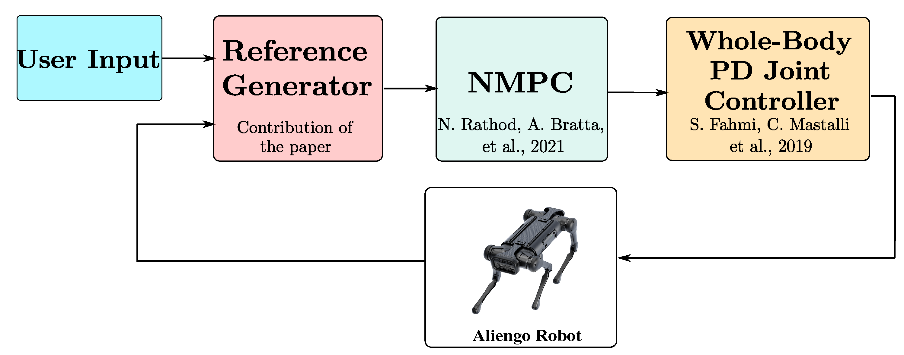
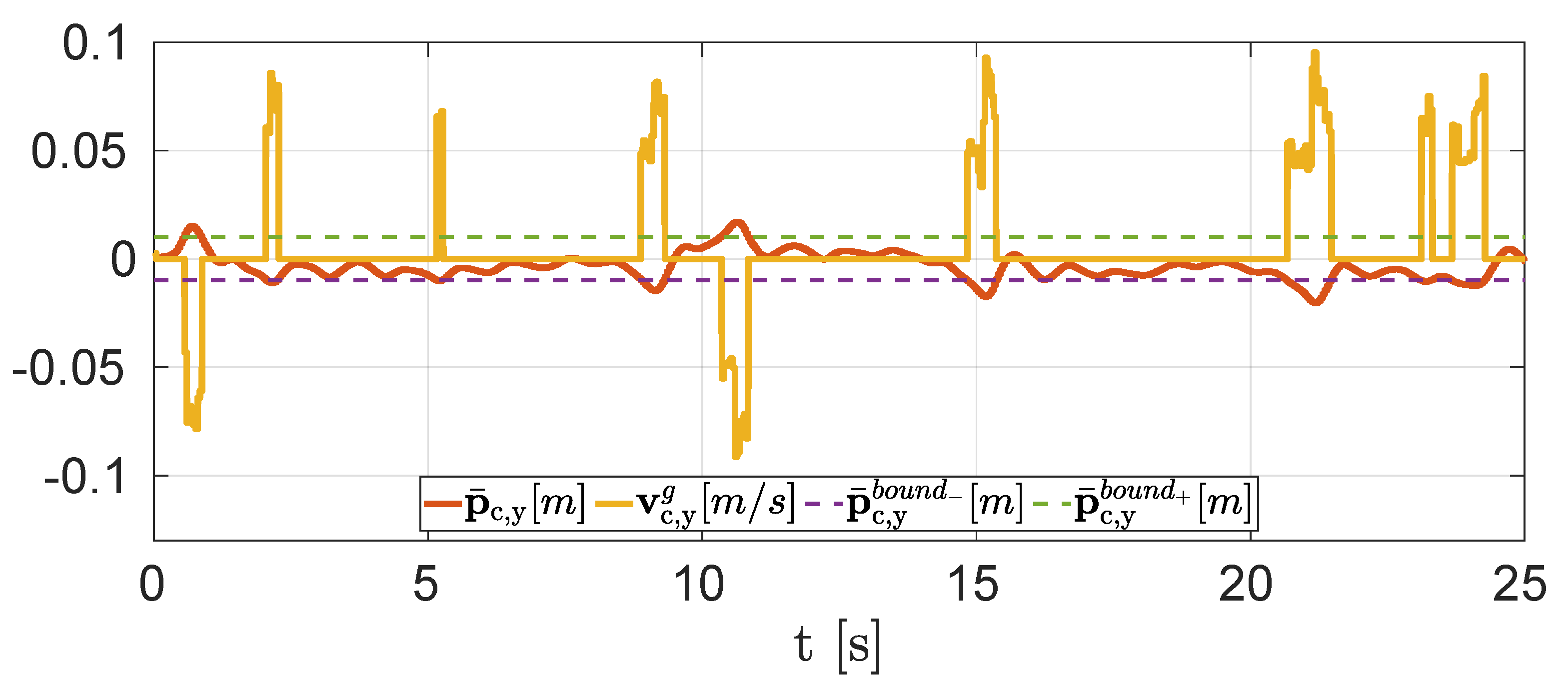
  • the presentation of a novel reference generator that drives the robot to accomplish a task (optionally in a user-defined time interval), taking into account the underactuation of statically unstable gaits, like the trot. Footholds are heuristically computed to be coherent with the CoM motion, and optimized GRFs are obtained in order to follow those trajectories. The formulation is lightweight enough to maintain the replanning frequency of 25 Hz of the NMPC;
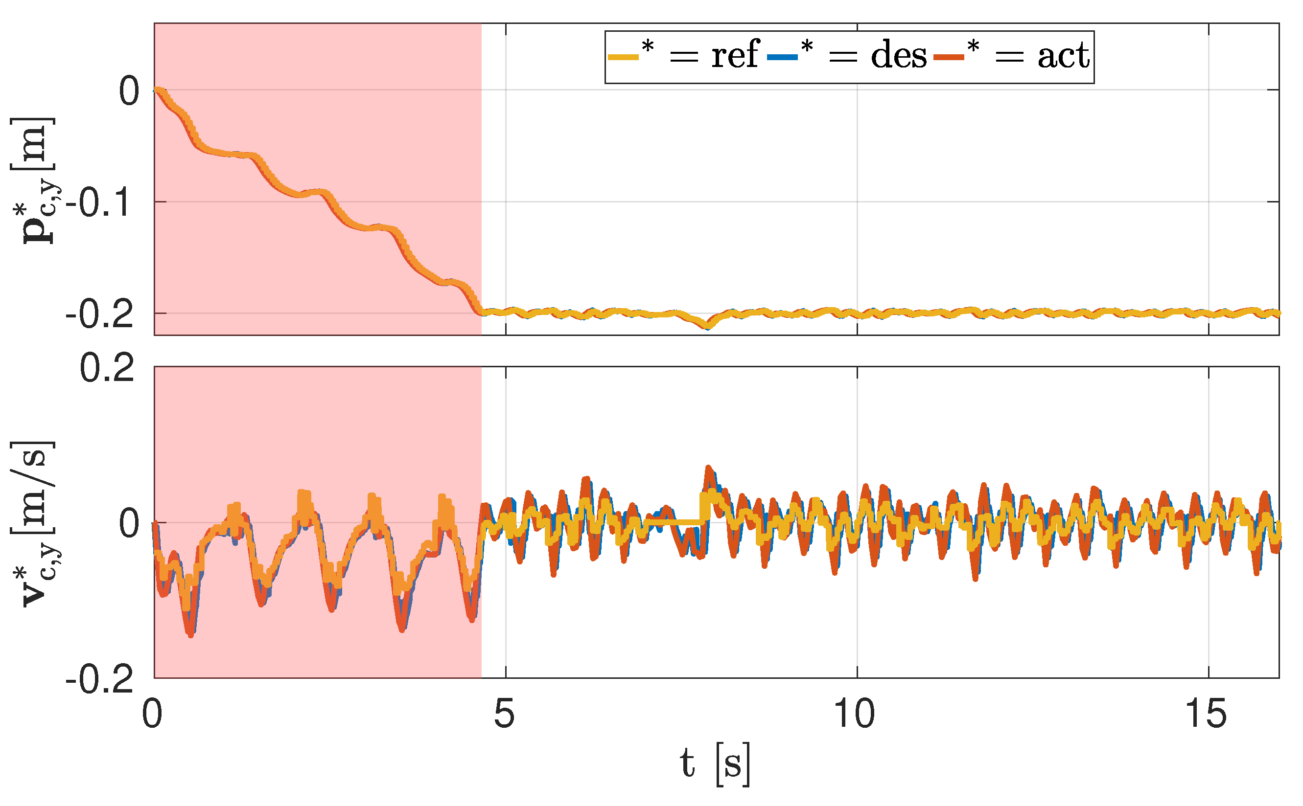
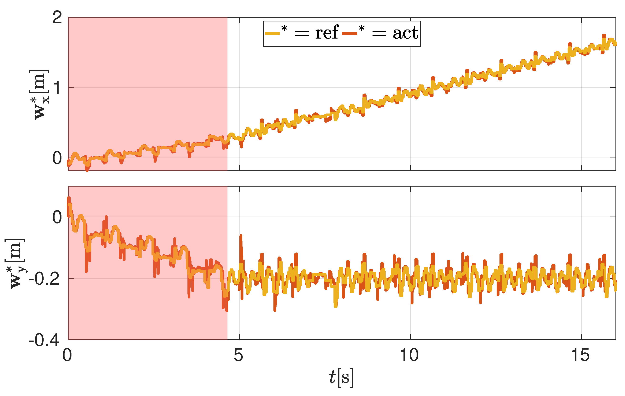
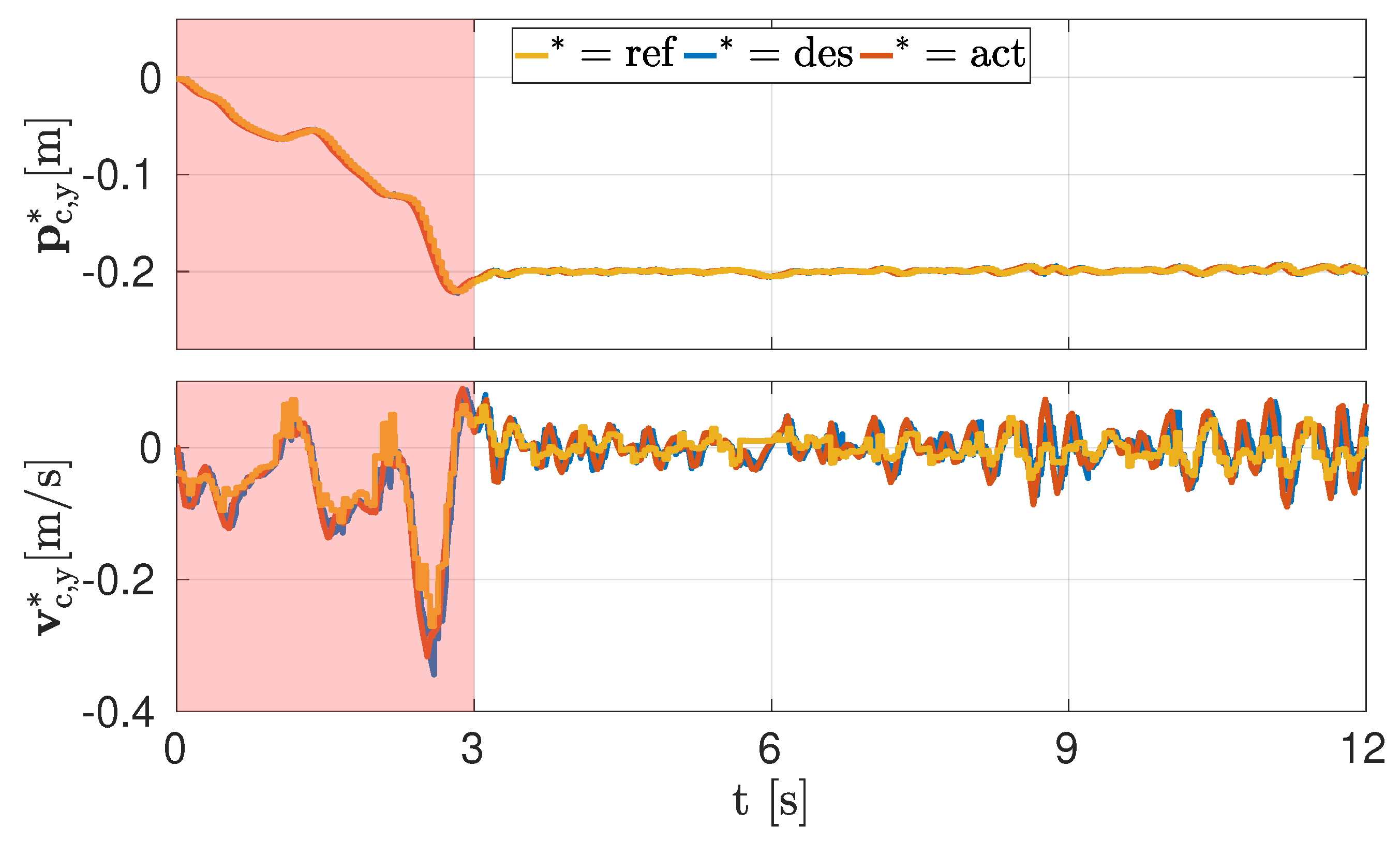
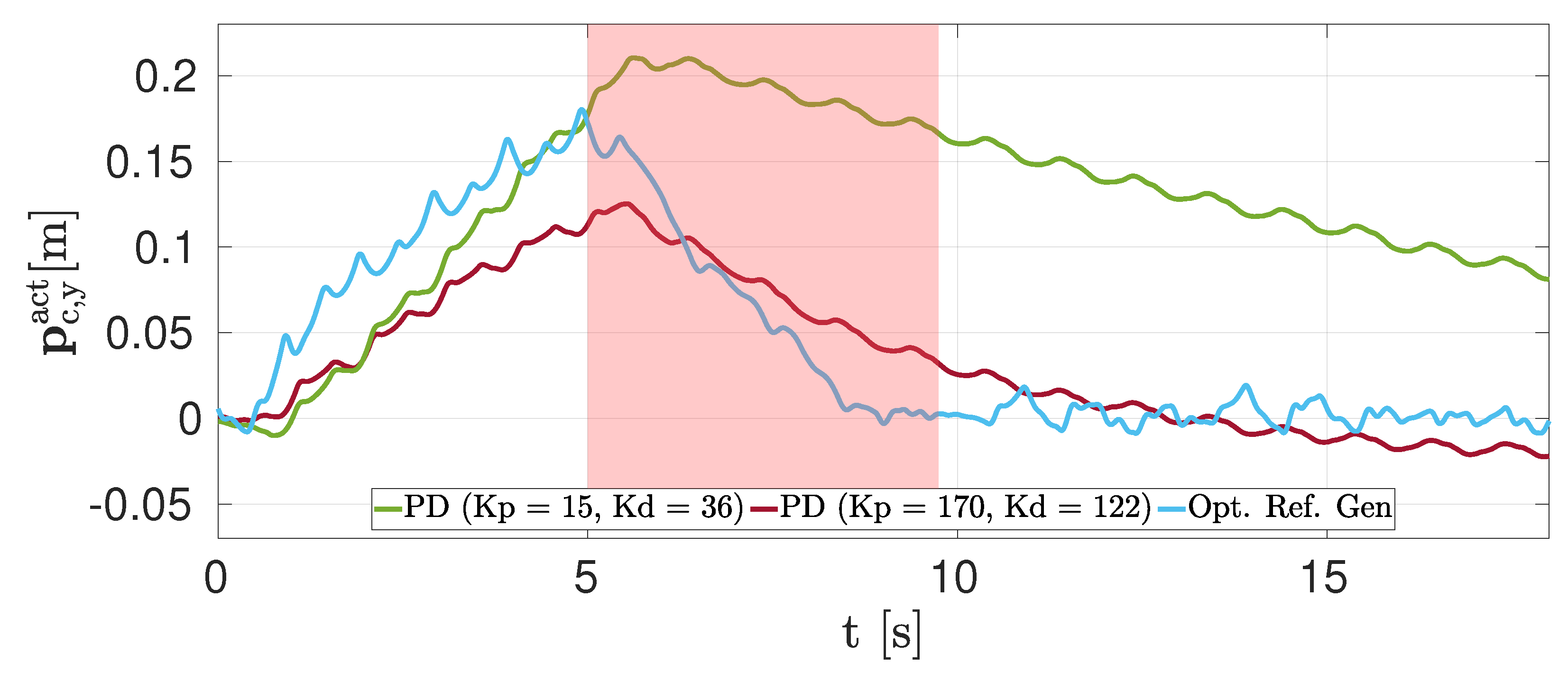
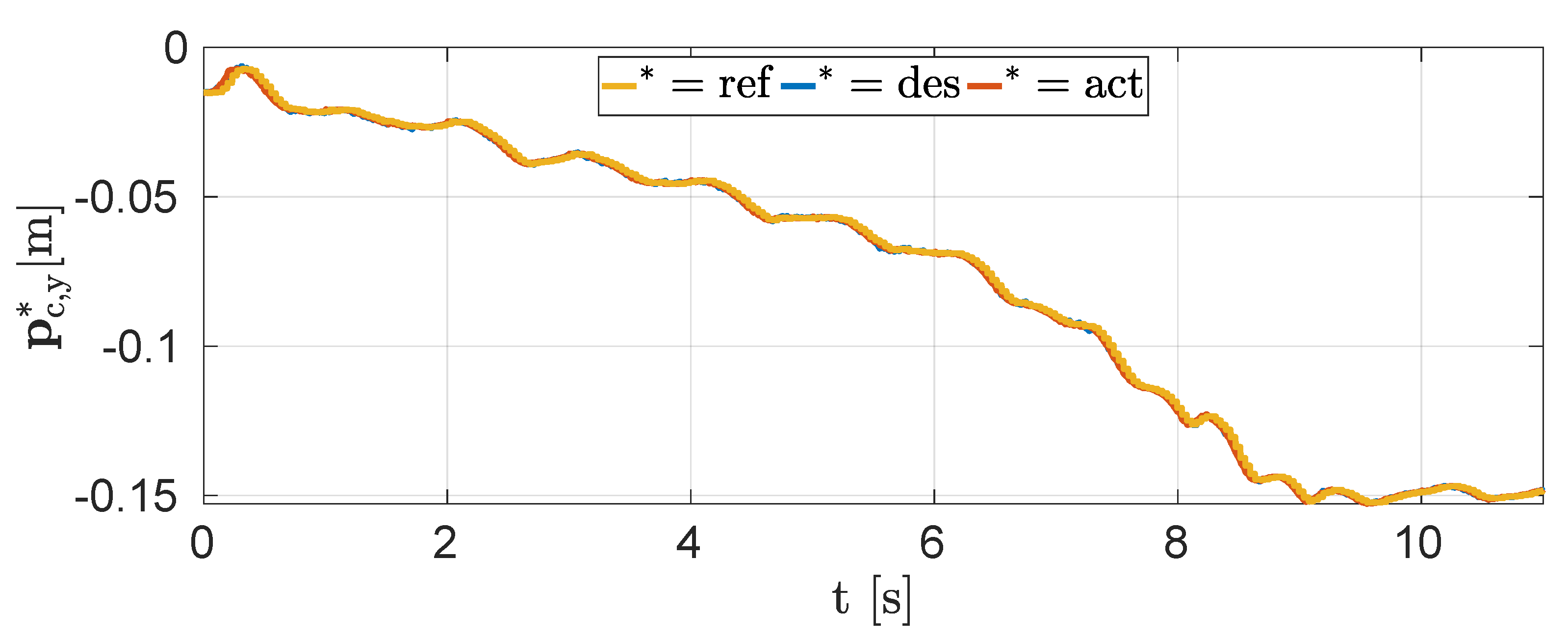
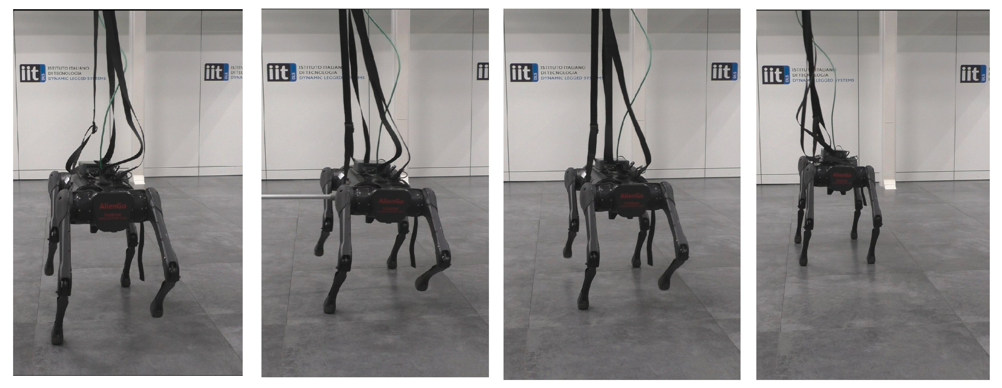
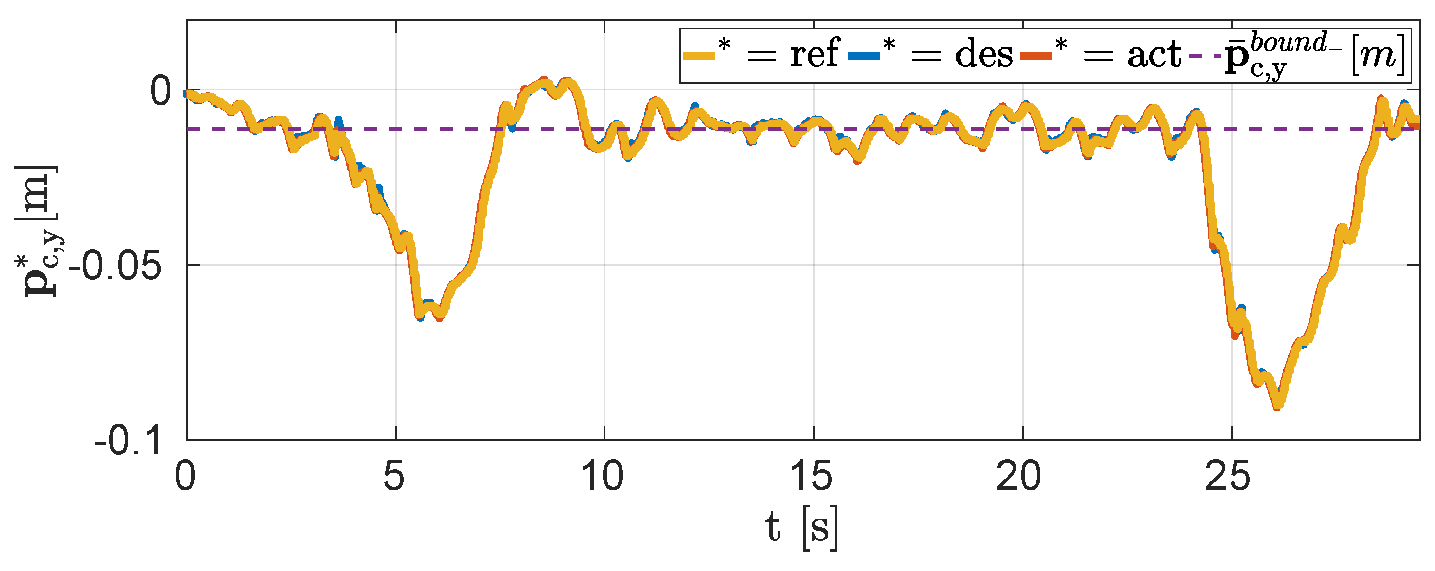
  • simulations and experiments to demonstrate the effectiveness of the proposed approach in three different scenarios: (a) straight motion, (b) fixed lateral goal, and (c) recovery after a push. We also compared in simulation our algorithm with a state-of-the-art approach (NMPC + PD action) for the scenario (c); and
  • as an additional minor contribution, we demonstrate the generality of the approach, showing it was able to deal with different dynamic gaits, i.e., trot and pace.

1.3. Outline

The paper is organized as follows: Section 2 gives an overview of our planning framework, highlighting the main features of the reference generator. Section 3 describes the optimization problem with the LIP model and how it is used to compute CoM position velocity and GRFs references. Simulations and experiments with our Aliengo [25] robot are presented in Section 4. Finally, we draw the conclusions in Section 5.

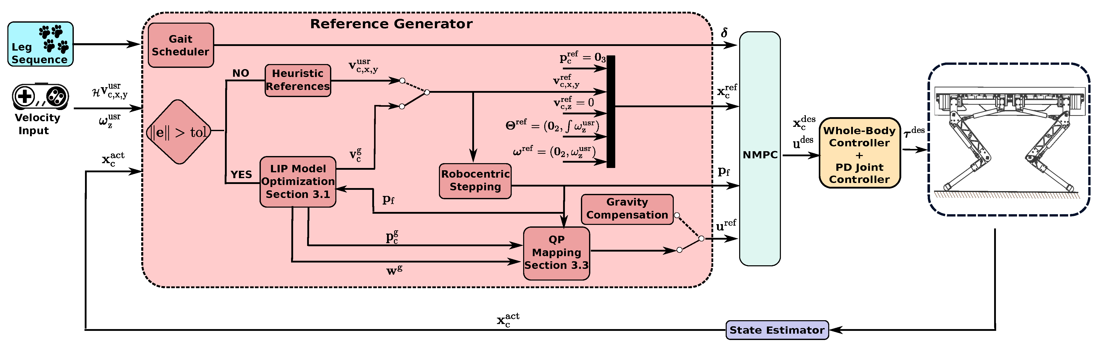
2. Locomotion Framework Description

Figure 2 gives an overview of our entire locomotion framework. The user decides the leg sequence and the values of both linear v c usr R 2 CoM reference velocity and heading ω z usr R reference velocity, i.e., the velocities that the robot should follow. The velocities can be changed during the motion and the NMPC will immediately react accordingly. In this work, we use two modules already presented in [5]: the gait scheduler and the robocentric stepping (also used in [26]).
Given the user-defined leg sequence, the gait scheduler returns the gait status (either swing or stance) δ i , k R of each leg i and for each time instant k in the reference horizon N g , reconciliating it with the real condition of the robot, e.g., early or late touchdown. The reference horizon N g corresponds to the maximum response time T f of the reference generator. Note that N g can be different from the horizon N used in the NMPC, with N g N . We use the symbol δ R 4 × N g to refer to the entire sequence of gait status. The robocentric stepping module, on the other hand, has the important task of computing footholds for each leg over the entire horizon. We use the symbol p f R 12 × N g to denote these quantities for the whole horizon.
The key idea of robocentric stepping is that the touchdown points are computed with respect to the hip position and they are offset, with respect to that, depending on the CoM reference velocity. Applying the robocentric stepping with the optimized reference velocities allows us to obtain the coherence between CoM and footholds. Variables p f and δ are also used as parameters in the SRBD model of the NMPC. If the error between the goal and average CoM position is lower than a threshold (see Section 2.1), the reference generator does not perform optimizations and user-defined velocities (heuristic references) are used as references also for the NMPC. We refer to this condition as the heuristic reference generator.
Instead, when the reference generator is in the optimize state, the sequences p f and δ are the input parameters to a first-stage optimization that employs the LIP model (Section 3.1). Here we compute the optimal X-Y CoM trajectory p c g , v c g to reach the goal p c goal , where dynamic stability is satisfied (i.e., ZMP always inside the support polygon). However, because the footholds are computed the first time with the simple heuristic approach, we need to recompute them by using the optimized velocity. This will result in a new set of footholds that will be used as inputs for a second optimization. We iterate this until a stop condition is reached, e.g., the maximum number of iterations or difference between two consecutive solutions below the defined threshold. As a safety check, if, instead, the solver is not able to converge to a feasible solution, the reference generator is set back to the heuristic status and v c usr /gravity compensation are used as references.
The CoM velocity trajectory v c g computed by the LIP model optimization is then used as velocity reference for the NMPC. As described in [5], reference CoM position, roll and pitch are not tracked, and the reference for the yaw is obtained by integrating the user-defined yaw rate ω z usr . We use the variable Θ ref R 3 to indicate the references for roll, pitch, and yaw. A Quadratic Program (QP)-based mapping (Section 3.2) computes the references for the GRFs u ref R 12 × N .
Finally, the output of the NMPC are the CoM trajectories (position, orientation, linear and angular velocities) x c des R 12 × ( N + 1 ) (as explained in [5] we parameterized the orientation with Euler angles, hence, the state dimension is 12) and GRFs u des R 12 × N that will be sent to the controller block. The controller is composed of a 250 Hz Whole-Body Control (WBC) [24] and a 1 kHz PD-joint controller. They generate the torque references τ des for the low-level joint controller of the robot. The state estimator module [27] provides the actual values x c act of the robot at a frequency of 500  Hz .

2.1. Goal Setting and Status of the Reference Generator

As already explained in Section 1, the robot cannot follow a user-defined velocity in the presence of non idealities or external disturbances, the case of a fixed goal corresponds to a scenario in which v c usr , y = 0 ) due to the MPC transparency. For this reason, we define the goal p c goal as the position the robot would have reached if it had followed the user-commanded velocities v c usr R 2 . The goal is updated at each iteration of the NMPC. It is initialized with p goal = p c , x , y act + N g v c usr T s at the beginning of an experiment and at each iteration it is incremented by v c usr T s . Variable T s is the sampling time of the reference generator and it is equal to 1 / f s where f s is the planning loop frequency. For the sake of simplicity, we assume that the sampling time T s of the NMPC and the reference generator are the same. As an alternative, the user can decide a fixed goal, either for one coordinate or both. A SLAM algorithm [28,29] goes beyond the scope of this paper, so we assume that there are no obstacles and the goal can be reached.
In order to change the status of the reference generator from heuristic to optimize in a meaningful way (e.g., no transition with the normal sway of the robot) we consider the average p ¯ c of the X-Y CoM position during the last gait cycle. To the average position, we add the offset due to the desired motion in the horizon N g and compare it with the goal. We compute the error as: e = p c goal p ¯ c + N g v c usr T s and when its norm e goes beyond a threshold when the reference generator status is set to optimize. Using Euclidean distance is a standard approach, but any other options, e.g., L1 or L could have been valid alternatives.
Algorithm 1 illustrates the pseudocode of the different computation phases of the reference generator.
Algorithm 1 Reference generator
 1:
Reference Generator status ← HEURISTIC 
 2:
e p c goal p ¯ c 0 N g T s v c usr d t
 3:
if e > t o l then
 4:
    Reference Generator status ← OPTIMIZE
 5:
end if
 6:
p f , δ Heuristic   References
 7:
if OPTIMIZE Reference Generator then
 8:
     while stop condition is not reached do
 9:
          v g LIP   Model   Optimization ( p c goal , x c act )
10:
         p f Robocentric   Stepping ( v c g )
11:
    end while
12:
    if LIP Model Optimization found feasible solutions then
13:
         v ref v g
14:
         u ref QP   Mapping ( p c g , w g , p f )
15:
    else
16:
         v ref v usr
17:
         u ref Gravity   Compensation
18:
    end if
19:
else
20:
     v ref v usr
21:
     u ref Gravity   Compensation
22:
end if
23:
p c goal p c goal + v c usr T s
24:
solve the NMPC [5]

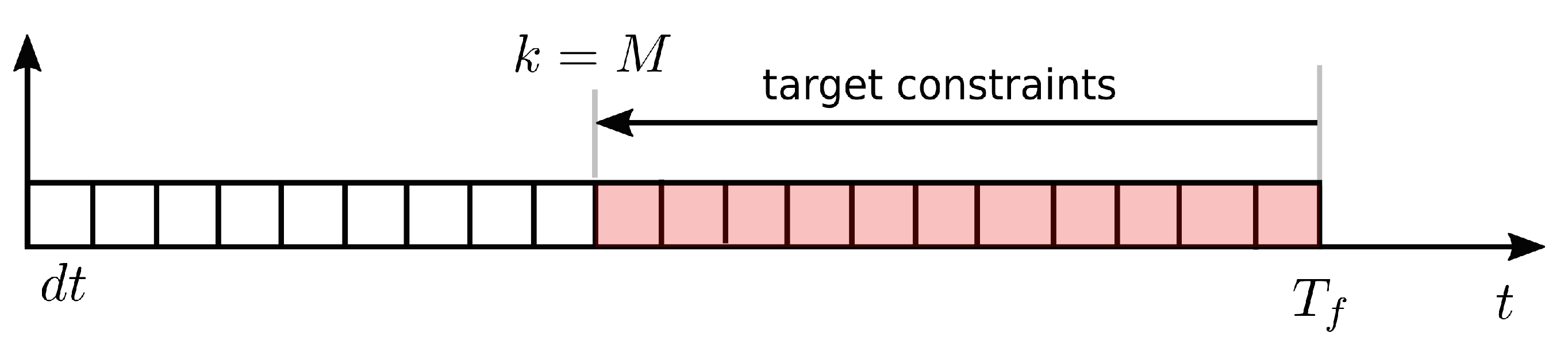
2.2. Formal Guarantees on Response Time

In an optimization problem, if we set the tracking of the goal as either a running cost or a terminal cost, the response will depend on the tuning of the weights of the cost itself. In addition, with this approach, we cannot impose a predefined time T f in which the robot reaches the goal (response interval). For these two reasons a hard constraint to impose that the CoM position matches the goal can be added to guarantee a response interval equal to T f , starting from the first time instant when the reference generator is set to the optimize status. Note that the size of the horizon N g will be linked to the response time T f ; therefore there will be a maximum value of T f that can be achieved by the reference generator, related to the real-time constraint posed by the re-planning frequency f s . This will depend on the computational power of the machine where the optimization is run. We also need to impose the same hard constraint on all the samples after M = T f / T s . Indeed, at every iteration of the NMPC, the interval without constraint should shrink because otherwise the target would never be reached (see Figure 3). For this reason, we enforce hard constraints on the goal, with the number of samples M that gradually reduces to zero. In this way, we ensure reaching the goal in a time that does not depend on the tuning of the weights. In practice, using hard constraints might lead the optimization to be trapped in an infeasible solution [30]. Therefore, an implementation with slack variables in the constraints, which allows us to relax them, is preferable. By penalizing their value in the cost function of problem (2), we have the guarantee that the robot reaches the target in a predefined time interval, and if this is not possible, the solver will find the best feasible solution.

3. Optimized Reference Generator

As already mentioned, the task of the reference generator is to compute along a horizon N g the linear (i.e., longitudinal and lateral) CoM velocity reference trajectories v c g to reach a desired goal/recover from an external disturbance in a predefined time T f and the trajectory of GRFs u ref to follow it.

3.1. LIP Model Optimization

One of the features of the proposed reference generator is to take into account the intrinsic underactuated nature of a robot when only two feet are on the ground [31]. Therefore, we employ the simplest model that is able to capture this underactuation: the LIP model [21]. Indeed, this allows us to compute the optimal trajectory for the CoM, while imposing a desired behavior for the ZMP. The ZMP is defined as “a point on the ground at which the tangential component of the moment generated by the ground reaction force/moment becomes zero” [32], and its position determines the direction and magnitude of the CoM acceleration. Guaranteeing that the GRFs are such that the resulting ZMP is inside the support polygon ensures that they also satisfy the unilateral constraints [33] (the legs can only push and not pull the ground); therefore, they can be effectively realized by a real robot. Because the support polygon boils down to a line connecting the stance feet during a two-leg-stance phase, the ZMP will be able to move only on that segment. Even though the ZMP-based models have been efficiently used in MPC approaches, e.g., [34], we are aware that the LIP model presents some assumptions (vertical and angular dynamics are neglected). As already mentioned, our NMPC uses the SRBD model that will consider these dynamics in the lower optimization stage.
We define the state of the reference generator x c g = { x c , 0 g , x c , N g g } R 4 × ( N g + 1 ) , with x c , k g = p c , k g , v c , k g T R 4 , the stack of X-Y CoM position, and velocity at time k . The control inputs are w g R 2 × N g = { w 0 g , w N g 1 g } , with w k g R 2 X-Y position of the ZMP at time k . Footholds p f , k and gait status δ k for all the feet at each sample k are the parameters used to compute the support polygon at each node of the reference horizon N g . Additional parameters are initial Z CoM position p c , z act and g R = 9.81 m / s 2 . To obtain x c g and w g , we cast the following optimization problem:
min x g , w g k = 0 N g p c , k g p c goal Q p 2 + v c , k g Q v 2 +
k = 0 N g 1 w k g w k ref Q w 2
s . t . x c , 0 g = x c , x , y act
x c , k + 1 g = x c , k g + v c , k g T s + T s 2 g 2 p c , z act p c , k g w k g g p c , z act p c , k g w k g T s
w k g S ( p f , k , δ k ) k I 0 N g 1 .
The terms (1a) and (1b) of the cost function aim to minimize the distance between CoM position and the goal, the norm of the velocities and the distance of the ZMP from the center of the support polygon w k ref (for robustness purposes). In addition, the minimization of velocity term (1a) prevents having large velocities that could determine footholds outside of the workspace of the leg due to the robocentric stepping. Matrices Q v R 2 × 2 and Q w R 2 × 2 are positive definite weighting matrices. The initial condition (1c) is expressed by setting x c , 0 g equal to the corresponding values x c act received from the state estimator. Equation (1d) corresponds to the discrete CoM dynamics for the LIP model. Equation (1e) imposes that the ZMP always lies inside the support polygon S ( p f , k , δ k ) . The symbol I 0 N g 1 indicates the set of integer numbers in the closed interval [0, N g 1 ].
The optimization problem (1) does not have any guarantee on the response time. As already discussed in Section 2.2, a formulation with a slack variable can be used to impose a predefined instant in which the robot has to reach the target:
min x g , w g , s k = 0 N g v c , k g Q v 2 + k = 0 N g 1 w k g w k ref Q w 2 +
k = 0 N g s k Q s , q 2 + Q s , l s k
s . t . x c , 0 g = x c , x , y act
x c , k + 1 g = x c , k g + v c , k g T s + T s 2 g 2 p c , z act p c , k g w k g g p c , z act p c , k g w k g T s
w k g S ( p f , k , δ k ) k I 0 N g 1
s k , x s k , y | p c , x , k g p c , x goal | | p c , y , k g p c , y goal | k I M N g
s k , x , s k , y 0 k I 0 N g .
The slack variable s k R 2 × 1 is added in the cost term (2b) and thanks to Equations (2f), and (2g) it allows us to impose that the robot CoM coincides with the goal after M samples. In contrast to the optimization problem (1), the cost function does not explicitly include a position term, because it is enforced with slacks into Equation (2b). Matrices Q s , q R 2 × 2 and Q s , l R 1 × 2 are the additional weights for the quadratic and linear term for the slack variables. Equations (2c)–(2e) are the same as Equation (1c)–(1e) respectively.

3.2. QP Mapping

The reference generator computes CoM trajectories which the NMPC must follow, but the latter also requires reference GRFs u ref R 12 × N . Because the output of the optimization problem (1) or (2) is a trajectory for the ZMP w g , we need to map this into a set of consistent GRFs, thus moving from a bidimensional to the higher dimensional space of contact forces. For this reason, we define the set of indices of the legs in contact with the ground by C . A parametric QP is solved to find the vector of GRFs u qp R 3 | C | , which corresponds to the ZMP location w g . If a foot is in the swing phase, its GRFs are set to 0 by default,
u i ref = u i qp i C 0 3 × 1 i C ,
where i is the leg index. Note that we need to solve a QP for each sample k in the horizon N, therefore to avoid overloading the notation, we do not specify the subscript k in the following quantities. The parameters of the model are the footholds p f , the X-Y components of the CoM position p c g , the ZMP trajectory w g , the initial Z CoM position p c , z act , and the mass of the robot m R . Thus, for every k we solve
min u qp u x , y qp Q u 2 + i C p f , i [ p c g , p c , z act ] T x u i qp Q k 2
s . t . w x , y g = i C p f i , x , y u i , z qp i C u i , z qp
i C u i , z qp = m g
g p c , z act ( p c g w g ) = i C u i , x , y qp m .
The first term of Equation (4a) is the regularization term on the X-Y components of the GRFs, with Q u R 2 × 2 as weighting matrix, whereas the second one minimizes the angular momentum rate, and it is weighted by Q k R 3 × 3 . Variable · x represents the skew-symmetric matrix associated with the cross-product. Equation (4b) is the definition of ZMP, Equation (4c) represents the gravity compensation. Equation (4d) guarantees that the X-Y CoM acceleration computed with the LIP model in the reference generator (left term) coincides with the one of the SRBD used in NMPC. It is worth highlighting that when the robot is on two legs, the ZMP lies on a line, and so it can only move in a 1D manifold. During that phase, imposing the Equation (4b) for the X component is enough to guarantee that the Y coordinate of the ZMP also respects the same constraint. Along the horizon N g , each problem is independent from the others, so they can be solved in parallel. In this way the computation effort remains low (a couple of ms to solve a QP problem with linear constraints) and therefore the new reference generator can be integrated into our high-frequency NMPC scheme.

4. Simulation and Experimental Results

The optimization-based reference generator endows the NMPC planner with the capability of recovering from disturbances and avoiding drifting in the face of nonidealities. To show its effectiveness, we tailored three template scenarios: (a) motion along a straight line, (b) reaching a fixed goal, and (c) recover from external pushes. We performed the simulations and experiments on the 22 kg quadruped robot AlienGo of Unitree.
We consider the trot as a template gait for our experiments because of its inherently unstable nature. Indeed, any asymmetry in the real robot can make it drift when setting a pure forward velocity. The quadruped is thus not able to follow a straight line.
The variable T s is set to 40 ms and the horizons of both reference generator ( N g ) and NMPC (N) are 50 nodes, corresponding to an interval of 2 s . We keep, thus, the same planning loop frequency of 25 Hz as our previous work. The trot parameters are cycle time T c = 1 s , duty factor D = duration of stance phase/ T c = 0.65. The values of the weighting matrices are reported in Table 1. Their value has been tuned with a trial and error procedure. We refer to Table 2 of [5] for the values of the weights of the NMPC and the WBC + PD Joint Controller. Without any lack of generalization, slack variables are considered only for the Y component.
We used the HPIPM [35] solver integrated into acados [36] library to find the solutions of the problem (2). The problem (4), instead, is solved by using eiquadprog [37], because it offers a more straightforward interface for the QPs. Both reference generator and NMPC run on an Intel Core i7-10750H CPU @ 2.60  GHz . The LIP model optimization takes 2–4 ms with the prediction horizon of 2 s and thus N equal to 50, whereas the time required by each QP (Equation (4a–4d)) is negligible, approximately 0.01 ms.
In this section, we will call the output of the reference generator as reference, the output of the NMPC as desired, and the real values measured by the state estimator as actual.

4.1. Simulations

The four-legged-stance phase in a walking trot is the only moment of the gait during which the robot has full control authority and is able to track the reference velocities. Neglecting this fact would lead to failure or unpredictably longer response times. In our algorithm, the reference generator already takes into account the underactuation, enabling us to deal with this issue successfully. The simulations of the scenario (a) are only reported in the accompanying video [38].
Figure 4 refers to the simulation of the scenario (b) in which the robot has to go to a lateral target ( 0.2 m on the Y coordinate) in a predefined time ( T f = 4.8 s ) and then keep it while walking. Because X-Y directions are decoupled in the LIP model, the X component of the goal p c , x goal is updated at each iteration of the NMPC according to Algorithm 1 and continuously tracked. The top plot demonstrates that the reference generator is able to compute reference CoM trajectories (yellow line) that allow the actual CoM values (red line) to accomplish the task. Because the reference quantities satisfy the underactuation of the gait, reference velocities are nicely tracked by the NMPC (respectively, yellow and blue line, bottom part of Figure 4) and consequently by the actual ones.
Figure 5, instead, shows the reference w g and actual X-Y components of the ZMP locations for the same simulation (computed by Equation (4b)). As can be seen, the robot is able to track the reference values for the entire cycle, for both X-Y coordinates, i.e., they have the same trend. In this simulation, we decided to keep the reference generator always in the optimize status to show how the algorithm is able to track (once the target has been reached) a zero user-defined lateral velocity v c , y usr .
Figure 6 reports scenario (b) with the same goal (−0.2 m ) but different response interval ( T f = 3 s ). Due to the smaller interval, the response is more aggressive and presents an overshoot which is then recovered within the 3 s interval. The task is achieved by simply modifying the response interval T f ; no tuning of the weights of the cost function is required. Shaded areas highlight the response interval. Figure 7 shows the tracking error between the actual and desired Y CoM position. It confirms that the error is negligible and the desired values are tracked by the robot.
Next, we want to validate our approach by comparing it with a simple Cartesian PD approach in the scenario (c). This is typically implemented computing a feed-forward force f ff , y R which depends on the error between the actual state and the goal, i.e., f ff , y = K p p c , y goal p c , y act + K d v c , y usr v c , y act .
In this scenario, for the first 5 seconds of the motion the robot is pushed with a force of 15 N in the Y direction. The user velocity v c , y usr is zero, so the task is to come back to the initial Y position. In Figure 8 we report the actual Y CoM position p c , y act in three different cases.
The green line represents the case in which the system is modeled as a second order with critically damped response.
From the control theory, we know that the settling time is equal to T f = 4 ζ ω n , with ζ equal to damping ratio and ω n natural frequency. To have a critically damped response we aim at ζ = 1.
Rewriting the second order equation of the mass/spring/damper as a function of ζ and ω n we have K p = m ω n 2 and K d = 2 ζ m K p .
Merging the two expressions results T f = 4 m K p with ζ = 1 . Considering T f = 4.8   s and a total robot mass m = 22 kg , we obtained K p = 15 N / m and consequently K d = 36 Ns / m .
It is evident that the CoM is far from reaching the goal in the predefined time.
The purple line, instead, represents the case in which the values of proportional and derivative gain are manually tuned such that the robot reaches the goal faster. The result is K p = 170 N/m and K d = 122 Ns / m . As can be seen in the plot, once the disturbance is removed, the robot moves toward the goal, but it is not able to follow it once it has been reached. In fact, the robot keeps drifting, moving away from the initial position. We can conclude thus that the approach with a feed-forward force results in a slow response, with a steady-state error with respect to the goal. The common practice of setting the PD parameters considering the system behaving as a second order system (i.e., spring/mass /damper) is not valid due to the underactuation, showing the limitation of the approach. In addition, even hand-tuning of the parameters does not allow the user to obtain the desired behaviour, e.g., the values of K p and K d which have good performance in recovering from the push (purple line) are not suitable for the straightforward motion. The result of our approach, instead, is reported with a light blue line. Once the disturbance has been removed, the reference generator computes a velocity trajectory that brings the robot toward the goal in the desired time T f (shaded area) and without steady state error.

4.2. Experiments

In this section, we present preliminary experiments for the scenarios (a), (b), and (c) carried out with the real robot platform. In these experiments, we employed the problem (1) without ensuring guarantees on the response time. As a first experiment, we performed scenario (a) on the robot, as illustrated in Figure 9.
The figure demonstrates that the NMPC with only a heuristic reference generator (dashed lines) does not succeed in moving on a straight line for a statically unstable gait as trot.
Indeed, the robot suffers lateral and backward (less visible) drifts for two reasons: (1) the trot being an unstable gait, the CoM always diverges between two four-legged-stance events in opposite directions. Any little asymmetry in the robot results in a cumulative drift in one direction; and (2) because Aliengo has c-shaped legs, they create nonzero moments about the pitch axis during a swing.
Enabling the optimal reference generator, instead, the robot is able to reach the goal and prevent the trajectory from drifting (see the continuous line in Figure 9).
Figure 10 shows the change in the reference lateral velocity (yellow line) done by the reference generator. When the average Y position ( p ¯ y , red line) exceeds the bounds ( p ¯ y bound , dashed lines), the status is changed to optimize and the reference generator brings back the CoM close to the goal. A threshold of 1 cm around the constant goal has been chosen for the activation. Once the goal has been reached, the reference generator automatically resets to heuristic, and the reference velocity becomes equal to the user one (zero). The continuous changing of the status of the reference generator demonstrates the need to have an external module which corrects the reference trajectories during a trot.
Figure 11 shows the Y position of the robot in the scenario (b) with a fixed goal of −0.15 m . As in simulation, the robot is able to track the reference value, due to the fact that the velocity takes into account the underactuation of the trot gait. In this case, we decided to keep the reference generator always set to optimize to demonstrate that it is able to work properly also when the target has been reached, compensating drifts as in scenario (a).
In the last experiment, we show how we can use our reference generator to react to external disturbances (see Figure 12). As we have already mentioned in the Introduction, the task is not to reject the disturbance, but to cope with it and later recover from its effect. An analysis of techniques to reject disturbances goes beyond the scope of this work. Figure 13 shows the Y position of the CoM in a real hardware experiment in scenario (c) when the robot receives two manually applied pushes. The threshold on the error is set to 1 cm (dashed purple line). During the push, the robot tries to resist to the disturbance and, thanks to the high-frequency re-planning of the NMPC, it is able to keep the stability and avoid falling. Once the pushing force is removed, the reference generator drives the robot back toward the initial position. As in the previous cases, the reference generator is set to optimize when the robot is diverging from the goal.
The readers are encouraged to check the experiments corresponding to the mentioned results in the accompanying video.

5. Conclusions

In this work, we presented a novel optimization-based reference generator for quadruped locomotion, which deals with the underactuation of statically unstable gaits and with external disturbances. It exploits the LIP model to compute feasible reference trajectories that allow the robot to accomplish a tracking task. A QP mapping is used to determine the GRFs which correspond to the ZMP location computed by the LIP model. Velocities and GRFs are used as informative tracking references by a 25 Hz lower-stage NMPC planner introduced in [5]. This results in the absence of conflicting tasks in the cost function, which simplifies the tuning of the weights inside the costs of the NMPC. We validated our approach by performing simulations and experiments with the 22 kg quadruped robot Aliengo in three different scenarios: (a) straight motion, (b) fixed lateral goal, and (c) recovery after a push. For the last scenario, we demonstrated that the simple solution of adding a Cartesian PD in parallel to the NMPC is not enough to return in a predefined time to the required position. In addition, we presented and validated in simulations a formulation with slack variables that are guaranteed to reach the goal in a specified time, without the need to further tune any parameters.
Future work involves extending the optimize reference generator also to the heading (i.e., yaw) orientation, and to perform additional experiments with the real platform with the formulation that respects a specified response time.

Author Contributions

The authors contributed to the paper in the following ways: Conceptualization, A.B. and M.F.; Formal analysis, A.B. and M.F.; Software A.B. and N.R.; Methodology A.B.; Investigation A.B. and M.F.; Visualization A.B.; Writing–original draft A.B.; Supervision M.F. and C.S.; Writing–review & editing M.F., N.R. and C.S.; Data Curation N.R.; Funding acquisition C.S.; Project administration C.S.; Resources C.S. All authors have read and agreed to the published version of the manuscript.

Funding

The publication was created with the co-financing of the European Union FSE-REACT-EU, PON Research and Innovation 2014-2020 DM1062/2021.

Acknowledgments

We thank Mario Zanon and Alberto Bemporad of IMT School for Advanced Studies Lucca for their precious advice and support.

Conflicts of Interest

The authors declare no conflict of interest.

Notation

Most commonly used symbols in this article.
N R NMPC horizon.
N g R Reference horizon.
δ R 4 × N g Sequence of gait status.
p f R 12 × N g Footholds sequence.
x c g R 4 × ( N g + 1 ) State of the optimized reference generator.
p c , k g R 2 X-Y COM reference position at time k.
v c , k g R 2 X-Y COM reference velocity at time k.
w k g R 2 ZMP position at time k.
s k R 2 × 1 slack variables at time k.
u qp R 3 | C | GRFs computed by the QP Mapping.
u des R n u × N Predicted GRFs by the NMPC.
x c des R 12 × ( N + 1 ) Predicted states by the NMPC.
x c act R 12 Actual robot state.
p ¯ c R 2 Average X-Y COM position.

References

  1. Raibert, M.H.; Tello, E.R. Legged Robots That Balance. IEEE Expert 1986, 1, 89. [Google Scholar] [CrossRef]
  2. Winkler, A.W.; Bellicoso, C.D.; Hutter, M.; Buchli, J. Gait and Trajectory Optimization for Legged Systems Through Phase-Based End-Effector Parameterization. IEEE Robot. Autom. Lett. (RA-L) 2018, 3, 1560–1567. [Google Scholar] [CrossRef] [Green Version]
  3. Bratta, A.; Orsolino, R.; Focchi, M.; Barasuol, V.; Muscolo, G.G.; Semini, C. On the Hardware Feasibility of Nonlinear Trajectory Optimization for Legged Locomotion based on a Simplified Dynamics. In Proceedings of the IEEE International Conference on Robotics and Automation (ICRA), Paris, France, 31 May–1 August 2020; pp. 1417–1423. [Google Scholar] [CrossRef]
  4. Li, H.; Wensing, P.M. Hybrid Systems Differential Dynamic Programming for Whole-Body Motion Planning of Legged Robots. IEEE Robot. Autom. Lett. (RA-L) 2020, 5. [Google Scholar] [CrossRef]
  5. Rathod, N.; Bratta, A.; Focchi, M.; Zanon, M.; Villarreal, O.; Semini, C.; Bemporad, A. Model Predictive Control with Environment Adaptation for Legged Locomotion. IEEE Access 2021, 9, 145710–145727. [Google Scholar] [CrossRef]
  6. Semini, C.; Tsagarakis, N.G.; Guglielmino, E.; Focchi, M.; Cannella, F.; Caldwell, D.G. Design of HyQ—A Hydraulically and Electrically Actuated Quadruped Robot. IMechE Part I J. Syst. Control. Eng. 2011, 225, 831–849. [Google Scholar] [CrossRef]
  7. Minniti, M.V.; Grandia, R.; Farshidian, F.; Hutter, M. Adaptive CLF-MPC With Application to Quadrupedal Robots. IEEE Robot. Autom. Lett. (RA-L) 2022, 7, 565–572. [Google Scholar] [CrossRef]
  8. Hong, S.; Kim, J.H.; Park, H.W. Real-Time Constrained Nonlinear Model Predictive Control on SO(3) for Dynamic Legged Locomotion. In Proceedings of the International Conference on Intelligent Robots and Systems (IROS), Las Vegas, NV, USA, 25–29 October 2020; pp. 3982–3989. [Google Scholar] [CrossRef]
  9. Amatucci, L.; Kim, J.H.; Hwangbo, J.; Park, H.W. Monte Carlo Tree Search Gait Planner for Non-Gaited Legged System Control. In Proceedings of the IEEE International Conference on Robotics and Automation (ICRA), Philadelphia, PA, USA, 23–27 May 2022; pp. 4701–4707. [Google Scholar] [CrossRef]
  10. Meduri, A.; Shah, P.; Viereck, J.; Khadiv, M.; Havoutis, I.; Righetti, L. BiConMP: A Nonlinear Model Predictive Control Framework for Whole Body Motion Planning. IEEE Trans. Robot. (T-RO) 2022. [Google Scholar] [CrossRef]
  11. Di Carlo, J.; Wensing, P.M.; Katz, B.; Bledt, G.; Kim, S. Dynamic Locomotion in the MIT Cheetah 3 Through Convex Model-Predictive Control. In Proceedings of the 2018 IEEE/RSJ International Conference on Intelligent Robots and Systems (IROS), Madrid, Spain, 1–5 October 2018; pp. 1–9. [Google Scholar] [CrossRef]
  12. Grimminger, F.; Meduri, A.; Khadiv, M.; Viereck, J.; Wuthrich, M.; Naveau, M.; Berenz, V.; Heim, S.; Widmaier, F.; Flayols, T.; et al. An Open Torque-Controlled Modular Robot Architecture for Legged Locomotion Research. Robot. Autom. Lett. (RA-L) 2020, 5, 3650–3657. [Google Scholar] [CrossRef] [Green Version]
  13. Barasuol, V.; Buchli, J.; Semini, C.; Frigerio, M.; De Pieri, E.R.; Caldwell, D.G. A reactive controller framework for quadrupedal locomotion on challenging terrain. In Proceedings of the IEEE International Conference on Robotics and Automation (ICRA), Karlsruhe, Germany, 6–10 May 2013; pp. 2554–2561. [Google Scholar] [CrossRef]
  14. Cebe, O.; Tiseo, C.; Xin, G.; Lin, H.C.; Smith, J.; Mistry, M.N. Online Dynamic Trajectory Optimization and Control for a Quadruped Robot. In Proceedings of the 2021 IEEE International Conference on Robotics and Automation (ICRA), Xi’an, China, 30 May–5 June 2021; pp. 12773–12779. [Google Scholar] [CrossRef]
  15. Bouyarmane, K.; Kheddar, A. On Weight-Prioritized Multitask Control of Humanoid Robots. IEEE Trans. Autom. Control 2018, 63, 1632–1647. [Google Scholar] [CrossRef] [Green Version]
  16. Bledt, G.; Kim, S. Implementing Regularized Predictive Control for Simultaneous Real-Time Footstep and Ground Reaction Force Optimization. In Proceedings of the IEEE International Conference on Intelligent Robots and Systems (IROS), Macau, China, 4–8 November 2019; pp. 6316–6323. [Google Scholar] [CrossRef]
  17. Bjelonic, M.; Grandia, R.; Geilinger, M.; Harley, O.; Medeiros, V.S.; Pajovic, V.; Jelavic, E.; Coros, S.; Hutter, M. Offline motion libraries and online MPC for advanced mobility skills. Int. J. Robot. Res. 2022, 41, 903–924. [Google Scholar] [CrossRef]
  18. Bemporad, A. Reference governor for constrained nonlinear systems. IEEE Trans. Autom. Control 1998, 43, 415–419. [Google Scholar] [CrossRef] [Green Version]
  19. Kolmanovsky, I.; Garone, E.; Di Cairano, S. Reference and command governors: A tutorial on their theory and automotive applications. In Proceedings of the 2014 American Control Conference, Portland, OR, USA, 4–6 June 2014; pp. 226–241. [Google Scholar] [CrossRef]
  20. Garone, E.; Di Cairano, S.; Kolmanovsky, I. Reference and command governors for systems with constraints: A survey on theory and applications. Automatica 2017, 75, 306–328. [Google Scholar] [CrossRef]
  21. Kajita, S.; Kanehiro, F.; Kaneko, K.; Yokoi, K.; Hirukawa, H. The 3D linear inverted pendulum mode: A simple modeling for a biped walking pattern generation. In Proceedings of the International Conference on Intelligent Robots and Systems (IROS), Prague, Czech Republic, 27 September–1 October 2021; pp. 239–246. [Google Scholar] [CrossRef]
  22. Orin, D.E.; Goswami, A.; Lee, S.H. Centroidal dynamics of a humanoid robot. Auton. Robot. 2013, 35, 161–176. [Google Scholar] [CrossRef]
  23. Mastalli, C.; Merkt, W.; Xin, G.; Shim, J.; Mistry, M.; Havoutis, I.; Vijayakumar, S. Agile Maneuvers in Legged Robots: A Predictive Control Approach. arXiv 2022, arXiv:2203.07554. [Google Scholar]
  24. Fahmi, S.; Mastalli, C.; Focchi, M.; Semini, C. Passive Whole-Body Control for Quadruped Robots: Experimental Validation Over Challenging Terrain. IEEE Robot. Autom. Lett. (RA-L) 2019, 4, 2553–2560. [Google Scholar] [CrossRef] [Green Version]
  25. Unitree Robotics. Available online: https://www.unitree.com/en/aliengo/ (accessed on 22 November 2022).
  26. Focchi, M.; Orsolino, R.; Camurri, M.; Barasuol, V.; Mastalli, C.; Caldwell, D.G.; Semini, C. Heuristic Planning for Rough Terrain Locomotion in Presence of External Disturbances and Variable Perception Quality. In Advances in Robotics Research: From Lab to Market; Springer Tracts in Advanced Robotics Series; Springer: New York, NY, USA, 2020; pp. 165–209. [Google Scholar] [CrossRef]
  27. Nobili, S.; Camurri, M.; Barasuol, V.; Focchi, M.; Caldwell, D.G.; Semini, C.; Fallon, M. Heterogeneous Sensor Fusion for Accurate State Estimation of Dynamic Legged Robots. In Proceedings of the Robotics: Science and Systems, Cambridge, MA, USA, 12–16 July 2017. [Google Scholar] [CrossRef]
  28. Durrant-Whyte, H.; Bailey, T. Simultaneous localization and mapping: Part I. IEEE Robot. Autom. Mag. 2006, 13, 99–110. [Google Scholar] [CrossRef] [Green Version]
  29. Nowicki, M.; Belter, D.; Kostusiak, A.; Cížek, P.; Faigl, J.; Skrzypczyński, P. An experimental study on feature-based SLAM for multi-legged robots with RGB-D sensors. Ind. Robot. 2017, 44, 428–441. [Google Scholar] [CrossRef] [Green Version]
  30. Hult, R.; Zanon, M.; Gros, S.; Falcone, P. Optimal Coordination of Automated Vehicles at Intersections: Theory and Experiments. IEEE Trans. Control. Syst. Technol. 2019, 27, 2510–2525. [Google Scholar] [CrossRef]
  31. Chignoli, M.; Wensing, P.M. Variational-Based Optimal Control of Underactuated Balancing for Dynamic Quadrupeds. IEEE Access 2020, 8, 49785–49797. [Google Scholar] [CrossRef]
  32. Harada, K.; Kajita, S.; Kaneko, K.; Hirukawa, H. ZMP analysis for arm/leg coordination. In Proceedings of the International Conference on Intelligent Robots and Systems (IROS), Las Vegas, NV, USA, 27 October–1 November 2003; pp. 75–81. [Google Scholar] [CrossRef]
  33. Vukobratovic, M.; Borovac, B. Zero-Moment-Point—Thirty five years of its life. Int. J. Hum. Robot. 2004, 01, 157–173. [Google Scholar] [CrossRef]
  34. Bellicoso, C.D.; Jenelten, F.; Gehring, C.; Hutter, M. Dynamic Locomotion Through Online Nonlinear Motion Optimization for Quadrupedal Robots. IEEE Robot. Autom. Lett. (RA-L) 2018, 3, 2261–2268. [Google Scholar] [CrossRef] [Green Version]
  35. Frison, G.; Diehl, M. HPIPM: A high-performance quadratic programming framework for model predictive control. IFAC-PapersOnLine 2020, 53, 6563–6569. [Google Scholar] [CrossRef]
  36. Verschueren, R.; Frison, G.; Kouzoupis, D.; van Duijkeren, N.; Zanelli, A.; Novoselnik, B.; Frey, J.; Albin, T.; Quirynen, R.; Diehl, M. Acados—A modular open-source framework for fast embedded optimal control. Math. Prog. Comp. 2021. [Google Scholar] [CrossRef]
  37. Guennebaud, G.; Furfaro, A.; Gaspero, L.D. Available online: https://github.com/fx74/uQuadProg (accessed on 22 November 2022).
  38. Video of the Experiments. Available online: https://www.youtube.com/watch?v=Jp0D8_AKiIY (accessed on 22 November 2022).
Figure 1. Overview of the locomotion framework. The reference generator presented in this work is integrated with the NMPC presented in our previous work [5]. The controller introduced in [24] allows the robot to track the trajectories computed by the NMPC. We used the quadruped robot Aliengo for the simulations and experiments.
Robotics 12 00006 g001
Figure 2. Block diagram of the proposed locomotion framework. Given the leg sequence, the user-defined velocities, and the actual state of the robot x c act , the reference generator computes the gait status δ , the footholds p f , the reference states x c ref , and GRFs u ref for the NMPC [5] at each control loop. If the norm of the error e between the goal and the average CoM position during the last gait cycle p ¯ c is smaller than the threshold, simple heuristic techniques are used (see [5]). In the other case, the reference generator is in the optimize status. CoM position and velocity to accomplish the task are computed with a LIP model; a QP mapping is used to obtain the GRFs corresponding to the ZMP computed by the LIP optimization. In addition, the CoM velocity is used to improve the footholds. Finally, the NMPC computes the optimal trajectories for CoM quantities x c des and GRFs u des . A whole-body controller and a PD-joint controller compute the optimal torques τ des that are sent to the robot. All Rights Reserved.
Robotics 12 00006 g002
Figure 3. Pictorial representation of the goal constraints enforced to achieve a certain response time T f . Pink blocks correspond to the nodes of the LIP optimization in which the constraint (2f) is active. At every iteration the variable M is decreased such that the time to reach the target matches the predefined time T f .
Robotics 12 00006 g003
Figure 4. Simulation, scenario (b): CoM Y position and velocity in a scenario in which the robot has to reach a target of −0.2 m , with a response interval of 4.8 s (120 iterations of the NMPC, pink blocks). Yellow lines are the output of the reference generator, which is used as reference for the NMPC. Blue lines correspond to the desired trajectories, tracked by the WBC. The red lines report the actual values.
Robotics 12 00006 g004
Figure 5. Simulation, scenario (b): X-Y ZMP location in a scenario in which the robot has to reach a target of −0.2 m along the Y direction with a response time T f = 4.8 s (120 iterations of the NMPC). The yellow line corresponds to the output of the reference generator, whereas the red has been computed by using Equation (4b).
Robotics 12 00006 g005
Figure 6. Simulation, scenario (b): CoM Y position and velocity when the robot has to reach a target of −0.2 m with a response interval of T f = 3 s . As in Figure 4, yellow, blue, and red lines correspond, respectively, to reference, desired, and actual quantities.
Robotics 12 00006 g006
Figure 7. Simulation, scenario (b): tracking error between actual and desired Y CoM position ( p c , y act p c , y des ).
Robotics 12 00006 g007
Figure 8. Simulation, scenario (c): comparison of the actual Y CoM positions between the PD force approach (green and purple lines) and our reference generator (light blue line). The goal is to come back to the initial position after a 15 N lateral push of 5 s . For the green line, the values are chosen to impose a response time of 4.8 s considering a second−order system response. For the purple line, instead, K p and K d are computed such that the system should have a critically damped response. In both cases, the robot is not able to converge to the goal. With our reference generator (light blue line) the robot recovers its initial position after the push, without any steady−state error.
Robotics 12 00006 g008
Figure 9. Experiment, scenario (a): Aliengo moving forward with zero lateral velocity set by the user. The dashed line represents the actual Y CoM position when the reference generator is forced to be always in heuristic status. The robot diverges from the goal of p c , y act = 0 and there is no part in the controller that brings it back. The continuous line shows the actual Y CoM position when the reference generator automatically changes its state according to the error e . Thanks to the corrections of the optimize reference generator, Aliengo is able to stay close to the goal.
Robotics 12 00006 g009
Figure 10. Experiment, scenario (a): Aliengo moving forward with zero user lateral velocity. The peaks in the reference velocity (yellow line) represent the moment in which the average Y position (red line) has passed the threshold (dashed lines) around the initial position and the reference generator is set to optimize status.
Robotics 12 00006 g010
Figure 11. Experiment, scenario (b): Aliengo robot reaches the target position of −0.15 m and then keeps moving following the user-defined velocity.
Robotics 12 00006 g011
Figure 12. Experiments, scenario (c), sequence of screenshots. The robot moves forward (picture 1), and is suddenly pushed with a stick (picture 2). Once the push is removed (picture 3), the optimized reference generator automatically drives the robot back to its initial position. Finally, the robot follows the user-defined velocity (picture 4).
Robotics 12 00006 g012
Figure 13. Experiment, scenario (c): CoM Y position of the robot. During the motion, the robot has been pushed twice and it automatically comes back to the initial position when the push is removed.
Robotics 12 00006 g013
Table 1. Weights used in the governor.
CostWeightValue
Velocities LIP Q v diag ( 200 , 300 )
ZMP Q w diag ( 100 , 350 )
Slack Q s , q diag ( 0 , 1000 )
Q s , l [ 0 , 1000 ]
Forces QP mapping Q u diag ( 100 , 100 )
Angular Momentum Rate Q k diag ( 1 , 1 , 1 )
Disclaimer/Publisher’s Note: The statements, opinions and data contained in all publications are solely those of the individual author(s) and contributor(s) and not of MDPI and/or the editor(s). MDPI and/or the editor(s) disclaim responsibility for any injury to people or property resulting from any ideas, methods, instructions or products referred to in the content.

