A Reconfigurable Parallel Robot for On-Structure Machining of Large Structures

Abstract

This paper presents a novel walking hybrid-kinematics robot that can be reconfigured to have three, five, and six degrees of freedom (DOFs) for adsorption machining of large structures. A symmetric 3PRPR or 3PRRR parallel mechanism with three translational (3T) DOFs is used to perform three-axis machining tasks. Three attachment pads connected to passive spherical joints are used to attach the robot to the surface of a large structure. Two or three rotational degrees of freedom can be added to the robot to adapt to a large structure’s irregular surface geometry and perform five- or six-axis machining tasks. This is achieved through modular reassembly or joint locking that reconfigures the robot from a three-DOF robot to a five- or six-DOF robot. A serial module providing two rotational DOFs can be added to the 3T parallel mechanism to provide five DOFs. A parallel module, namely 3SPR or 3SU mechanism, can be added to the 3T parallel mechanism to provide six DOFs. The mobility, pose kinematics, differential kinematics, singularities, and workspace of the 3SPR and 3SU parallel mechanisms alone and combined with the 3T mechanism are discussed in this paper. It is shown that the singularities of the mechanism can be easily avoided by making the moving platform of the 3SPR or 3SU mechanism smaller than the base, limiting the range of some joints, and having an appropriate length of the links. Furthermore, a method to optimize the workspace of the mechanism was also discussed.

1. Introduction

Large structures such as airplane and construction structures often need machining processes, including drilling. Robots have been used to perform those tasks to increase productivity and accuracy. Since the large structures are not practical and sometimes impossible to be moved, we need the robots to be mobile. To meet this need, there are already some existing mobile robots developed. However, many of them are based on serial ki-nematics which suffers from low compliance, particularly when the arms of such robots are significantly extended. In addition, these robots are often docked on ground when the machining tasks are performed. Hence, the rigidity of such robots when performing the machining tasks is compromised due to both the compliance of the serial robot arm and the compliance of the docking mechanism. To overcome this problem, we need a robot that is mobile and rigid at the same time. Added to these two criteria, we quite often need the robot to be able to move in confined spaces within the large structures. Hence, we also need the robot to have relatively small size. Although a serial robot can be mounted on a mobile base to be mobile, it cannot satisfy the rigidity and the small size at the same time. This is because the serial robot should be made bulky to have an acceptable rigidity. The three criteria can be satisfied by employing a parallel robot. To avoid the low compliance due to docking mechanism, on-structure parallel robots have been introduced. Such robots are attached directly to the large structures’ surface while performing a machining task to the structures’ surface. To change their positions, the robots also have locomotion capability. Various attachment methods such as magnetic and suction adhesion can be utilized to make the robot attach to large structures.

Among the developed on-structure robots are the walking hexapods [1,2,3] that require six actuators for manipulation and locomotion. A similar robot with a hybrid parallel mechanism that requires five actuators was also developed [4]. Meanwhile, typical legged robots to which direct attachment can also be potentially applied include quadrupeds and walking tree-like hexapod robots [5,6]. In addition, several legged robots in which the individual legs have parallel kinematics were also built [7,8,9,10,11,12,13,14,15].

A common drawback among the robots mentioned above is the use of many actuators, typically ranging from five to twelve. Although those robots can typically perform a five- or six-axis machining task with their many actuators, one often only needs a three-axis machining capability. In such a case, one should be able to use three actuators as a minimum to perform the task. For such a purpose, walking parallel robots with three degrees of freedom (DOFs), such as [16,17], were built. However, the use of such walking parallel robots is limited to only three-axis manipulation.

To provide flexibility in the type of machining tasks being able to be performed, including three-, five-, and six-axis machining tasks, this work proposes a novel on-structure robot that can be reconfigured to perform either a three-, five-, or six-axis machining task. The reconfigurability of the robot is achieved by modular reassembly or joint locking. With this reconfigurable design, one can optionally use a certain module based on the needs. For example, when only three-axis machining tasks, such as drilling perpendicular to a flat structural surface, are required, only the basic build of the robot with three actuators is needed. When a five- or six-axis machining is required, one can use the same robot with additional modules or DOFs. Hence, the advantage of the minimum number of actuators can be taken only when the basic build with three actuators is used. As soon as the additional modules or DOFs are used, the number of actuators turns to five or six, which is similar to some existing on-structure parallel robots.

Nevertheless, the proposed reconfigurable on-structure parallel robot has the following advantages in comparison with the existing on-structure parallel robots:

• Using reconfiguration by reassembly, we have a lighter robot when the basic build of the robot with three actuators is used. With other on-structure parallel robots having five or more actuators, the larger number of actuators results in larger weight. This is because such robots with five or more actuators have fixed topology, and hence, all their actuators should always be mounted on the robots although the robots are performing three-axis machining tasks.
• The modular design of the robot results in easier and less costly maintenance. When any additional module needs replacement, one can replace only that particular module, without a need to replace the whole robot. Replacement of such components is also easier due to the modular design.
• The modular robot can be sold as multiple packages using the same basic build. Each robot package is sold with its own topology and number of DOFs. The use of the same basic build for the various packages gives an advantage to the manufacturer in terms of the design, production, and sales. This is due to the modularity of the robot. On the user side, the purchase of the modular robot can be performed in multiple phases. One may start procuring the three-axis basic build with lower cost. This three-axis robot can already be used for three-axis machining tasks. At a later time, the additional modules can be procured when they are required.
• The joint motion planning in the three-axis motion, in both the reassembly and joint locking schemes, is simpler as the robot uses only three actuators. In contrast, other on-structure parallel robots with five or more actuators need to involve all of their actuators in the joint motion planning even when they are used for three-axis motion.

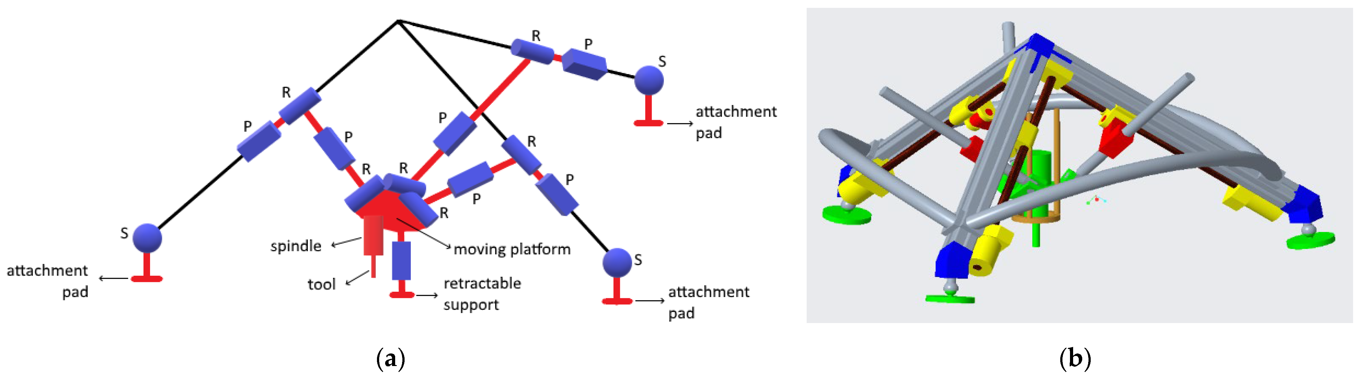
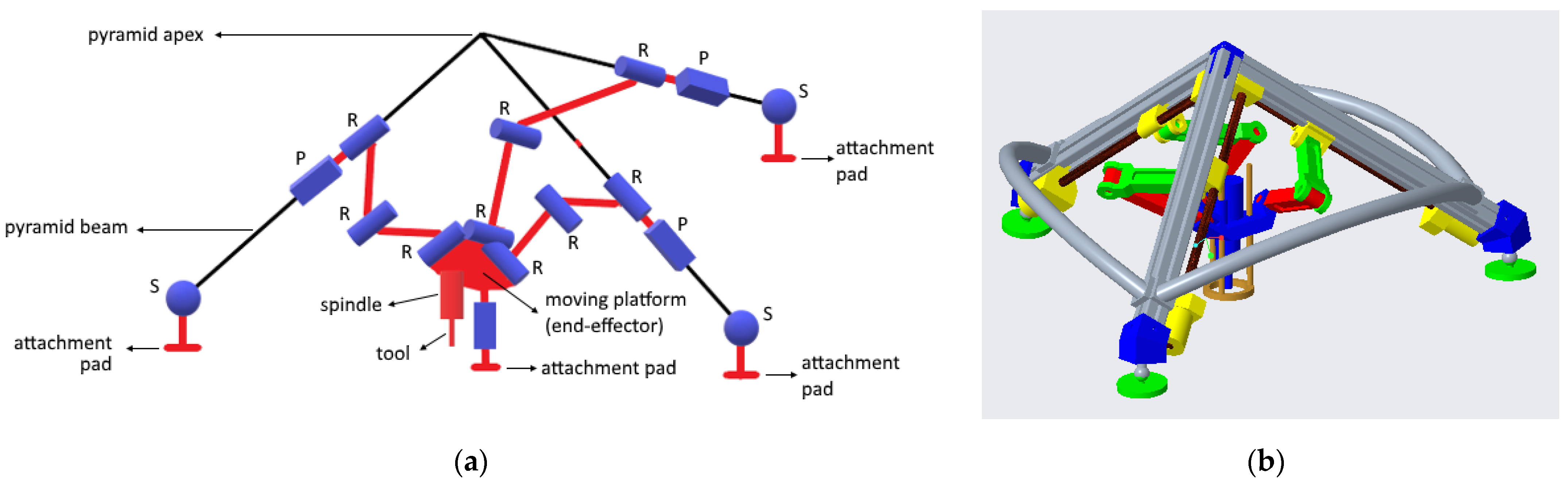
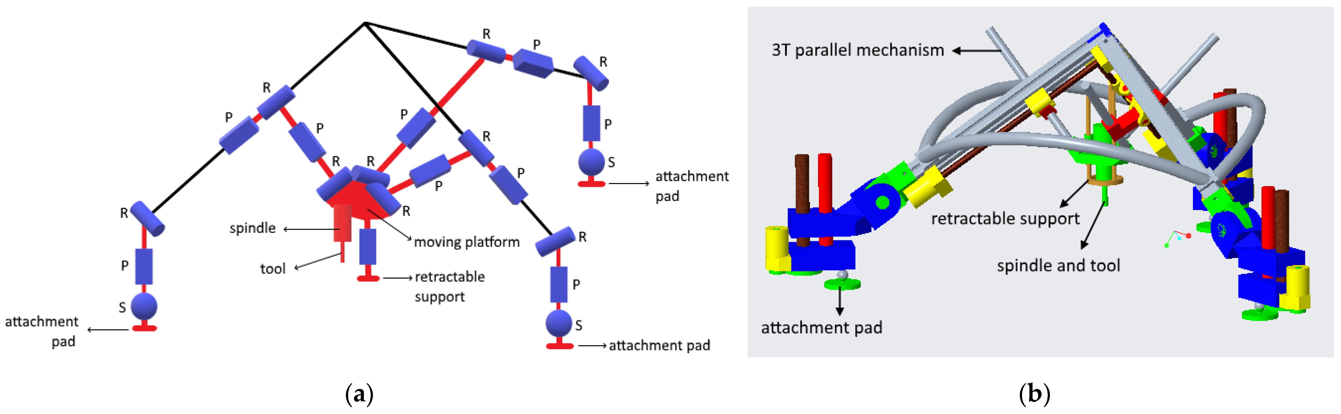
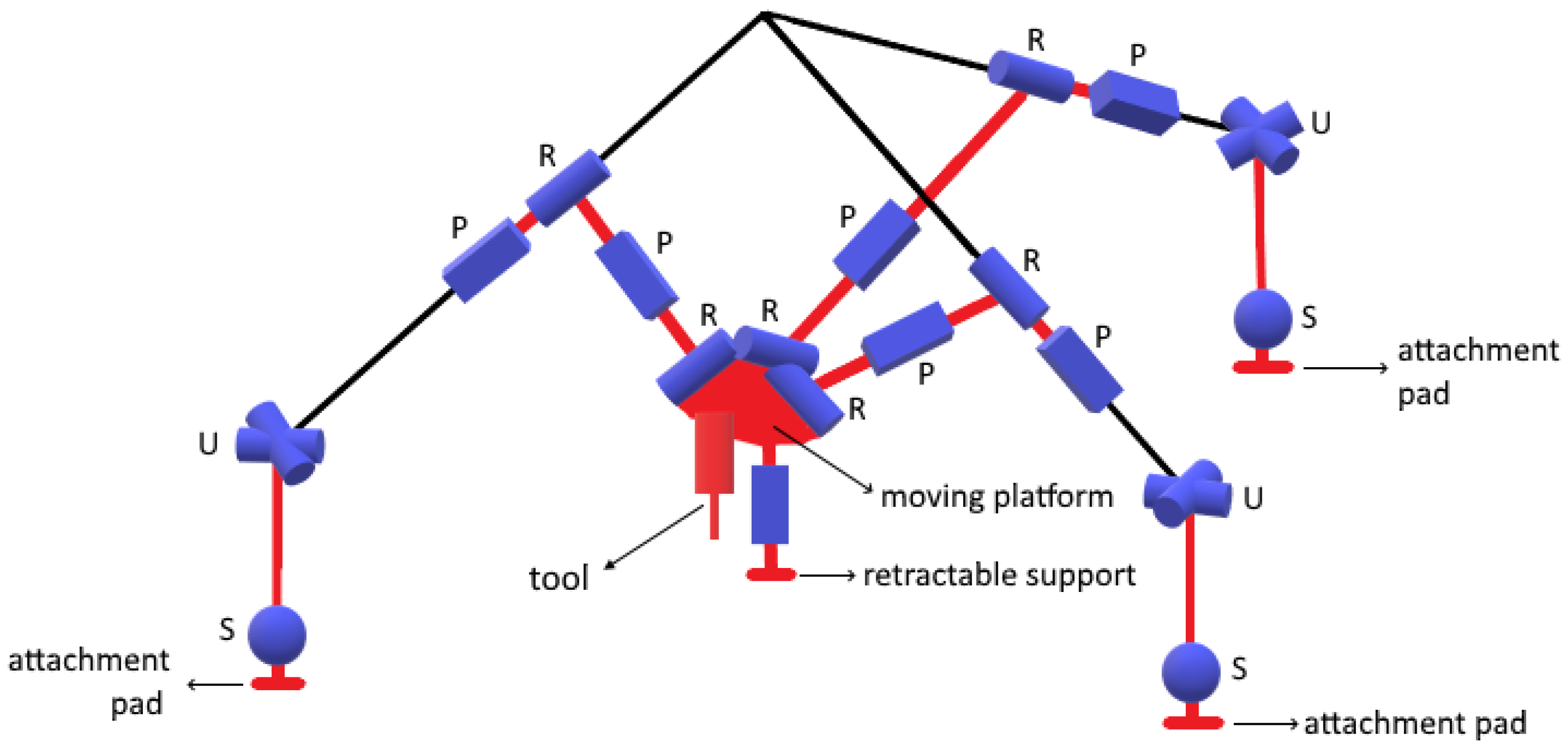
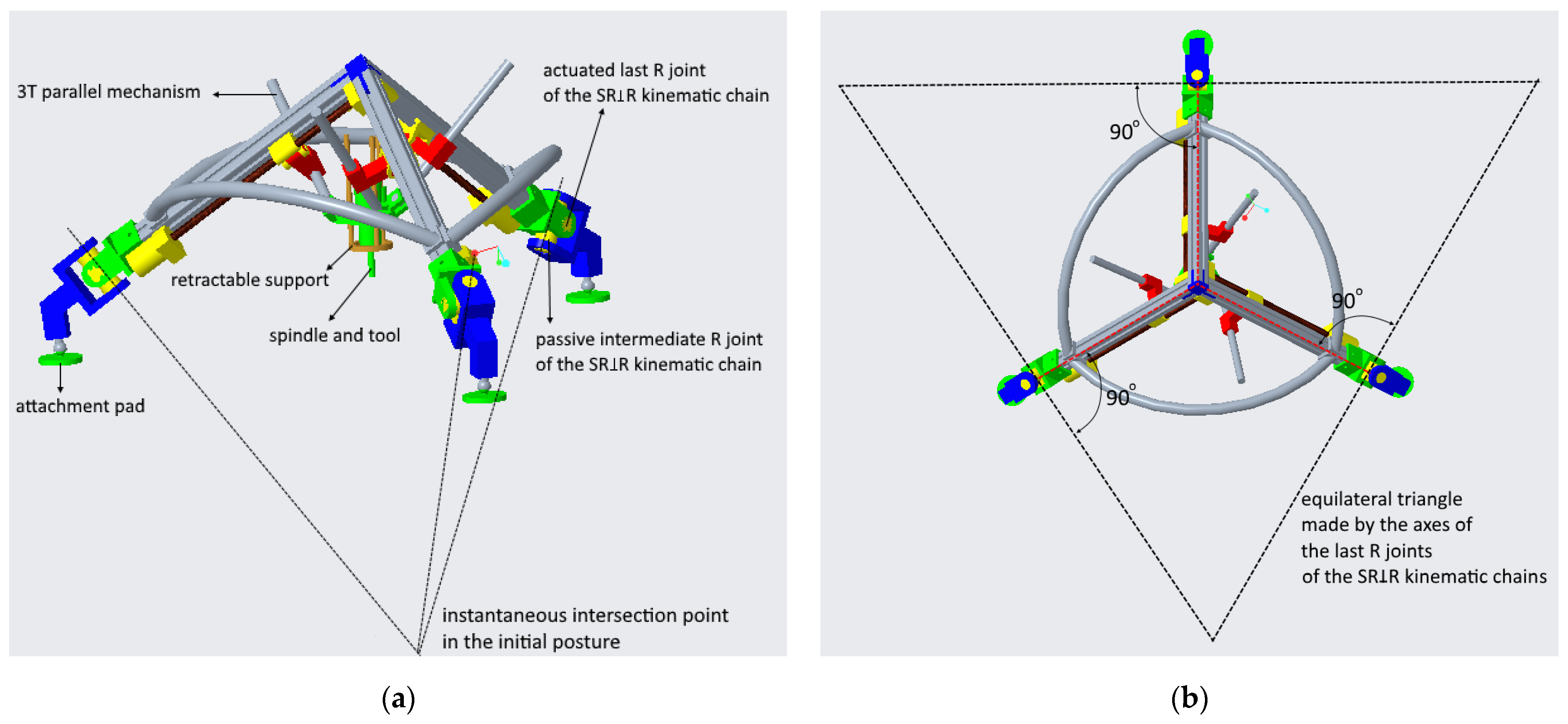
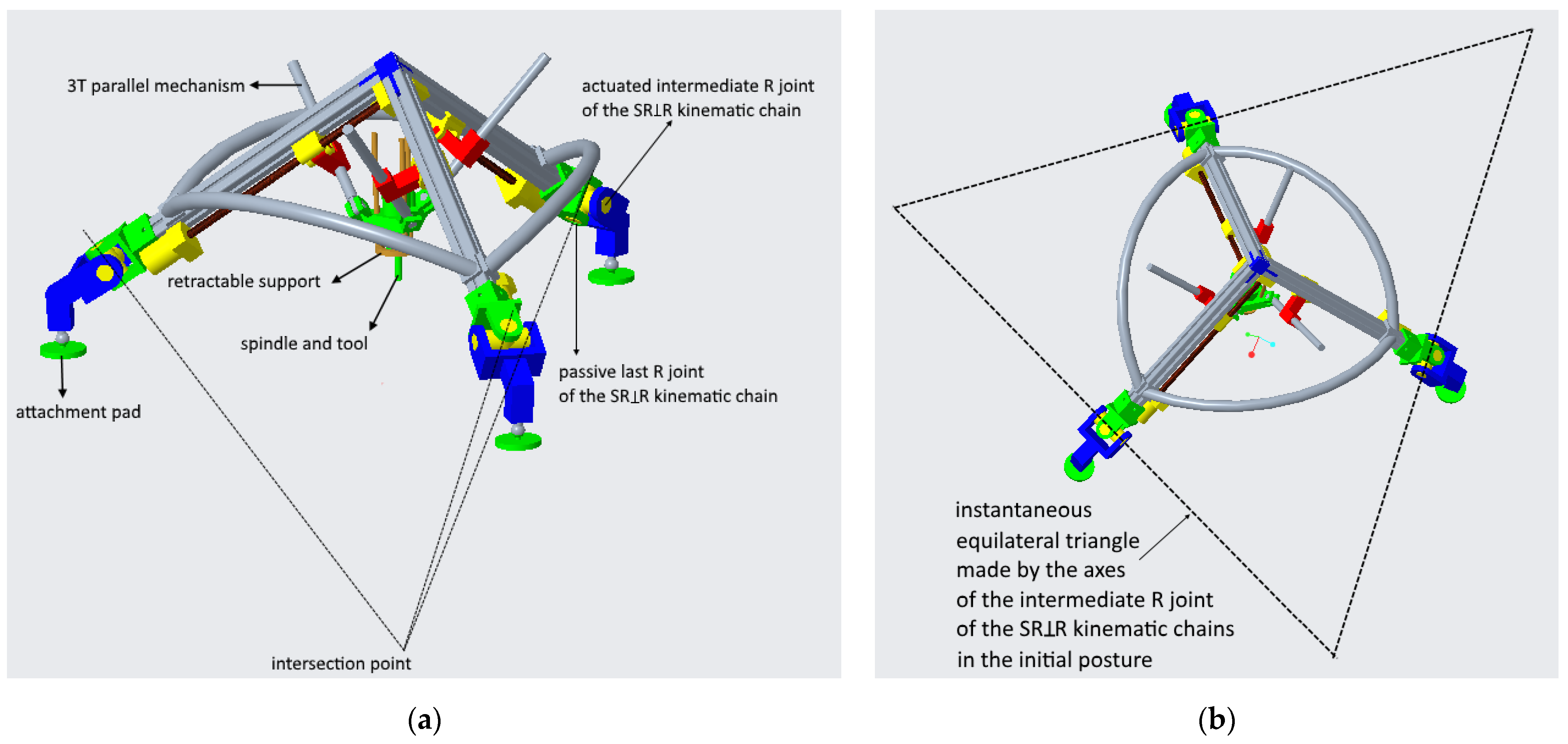
Hence, the contribution of this work is a novel reconfigurable design of an on-structure robot which enables the use of the robot for various types of machining tasks with weight adjustment capability through modularity, easier maintenance, lower design and manufacturing costs, modularity-based sales and procurement, and simpler three-axis motion planning.

Since the proposed design employs parallel kinematics with a typical drawback of limited workspace, this paper also discusses a method to optimize the workspace of the proposed robotic mechanism. As some performance measures of a parallel mechanism often contradict each other, a multi-objective optimization is often considered. There are three typical methods to handle the multi-objective optimization. The first is transforming the multiple objectives into a single objective with weights introduced to each objective; this is commonly called the weighted sum approach. The second is selecting the top-priority objective as the single objective while transforming the other objectives as the optimization constraints, such as in [18]. The third is implementing a Pareto optimality optimization such as in [19]; this provides multiple solutions ready for a designer to pick based on the designer’s preference. References [20,21] compared some of these various methods. The optimization method used in this work combines the first and second me-thods mentioned above.

The remainder of this paper is organized as follows. Section 2 discusses the topology of the robot. Section 3 analyzes the mobility of the parallel mechanisms. Section 4 discusses the pose kinematics of the mechanisms. Section 5 derives the differential kinematics of the mechanisms and subsequently discusses the singularities of the mechanisms. Section 6 discusses the workspaces of the mechanisms. Section 7 describes how the mechanism is reconfigured. Section 8 discusses an optimization method to maximize the workspaces of the mechanisms. Section 9 presents some design considerations. Finally, Section 10 concludes the paper. In this paper, the terms “structure” and “workpiece” are used interchangeably. For convenience, we provide the list of abbreviations and symbols used in this paper in Appendix A and Appendix B.

2. Topology

The proposed three-axis robot consists of a pyramid frame and a symmetric parallel mechanism that can be either a 3PRPR topology, as shown in Figure 1, or a 3PRRR topology, as shown in Figure 2. The number three indicates that the mechanism has three symmetric limbs, whereas the letters P and R represent the prismatic and revolute joints, respectively. Both topologies provide 3T end-effector mobility without any dependent rotational motion. In both topologies, the proximal P joints and all the R joints are parallel with the three segments of the pyramid frame. The ends of the three segments of the pyramid frame are attached to spherical joints. The spherical joints are attached to attachment pads which can be implemented using vacuum suckers, magnetic pads, or other adhesion/attachment technologies. The attachment pads are to be placed on the workpiece surface. The robot is attached to the workpiece surface when the attachment pads are activated. While the robot is attached to the workpiece surface, the 3PRPR or 3PRRR mechanism makes a 3T motion to perform machining tasks such as drilling a hole perpendicular to the workpiece surface. The whole topology of the robot can be named 3A+3S+3PRPR or 3A+3S+3PRRR, where A and S, respectively, indicate the attachment and the spherical joint, whereas the + sign indicates a serial connection. For the purpose of walking motions, a support equipped with an attachment feature is attached to the moving platform. This support can be retractable. It is retracted when the robot is performing a manipulation task; it is extended and attached to the surface of a workpiece/structure when the robot is making a walking motion. The walking motions are performed by manipulating the 3PRPR or 3PRRR mechanism while either the robot is pivoting about one attachment pad as the other two attachment pads are released or the robot is translating as the retractable support and the attachment pads are, respectively, engaged and released in turn. The detailed description and the kinematics of the walking motions are beyond the scope of this paper. However, this paper has a Supplementary Video showing the robot’s walking motions.

With the 3PRPR mechanism, the angle between two adjacent segments of the pyramid frame, in general, can be 90 degrees, less than 90 degrees, or more than 90 degrees. Making the angle 90 degrees gives several advantages, including a large workspace and moderate stability. With the 3PRRR mechanism, the angle between two adjacent segments of the pyramid frame must be 90 degrees to enable the mobility of the mechanism. Furthermore, in the 3PRPR mechanism, either the proximal or intermediate P joints can be actuated. When the 3PRRR mechanism is used, it is more practical to actuate the P joints. In the remainder of this paper, the illustration of both parallel mechanisms is represented by only one of them, the 3PRPR mechanism, for conciseness.

A typical application scenario is attaching a tool to the parallel mechanism’s moving platform to perform specific tasks such as drilling or milling. Suppose the surface of the workpiece is flat or a section of a spherical surface. In that case, either the 3PRPR or 3PRRR mechanism will automatically orient the tool perpendicular to the tangent of the workpiece surface, as illustrated in Figure 3. In the case where the surface of the workpiece is not flat or not a section of a spherical surface, it is no longer guaranteed that the tool’s orientation is perpendicular to the tangent of the workpiece surface. In such a case, the robot can be reconfigured by adding a module that adds two or three actuated rotational DOFs to compensate possible non-perpendicularity of the tool. In addition, the additional DOFs also provide five- or six-axis machining capability to the robot.

The first reconfiguration scheme is attaching a 2R module to the 3T moving platform, as illustrated in Figure 4. The 2R module can be a serial or parallel 2R module. The topo-logy of this scheme can be named 3A+3S+3PRPR+1RR or 3A+3S+3PRRR+1RR, depending on the 3T mechanism used. The transformation between the 3T and 3T2R robots is performed through reassembly or joint locking, which will be thoroughly discussed in Section 7.

The second reconfiguration scheme is adding a 3-DOF parallel mechanism that provides rotational mobility to the base of the 3T parallel mechanism. In other words, two parallel mechanisms, namely lower and upper parallel, are combined. In this scheme, the first joint in each limb of the lower parallel mechanism should be an S joint for modularity. The moving platform of the lower parallel mechanism serves as the base of the upper parallel mechanism. Hence, the whole mechanism is a 6-DOF hybrid-kinematics mechanism.

For the same reason, modularity, the lower parallel mechanism, should also be symmetric. Accordingly, two symmetric parallel mechanisms, namely 3SPR and 3SRꞱR (3SU), are proposed as the lower parallel mechanisms. The Ʇ sign in 3SRꞱR indicates that the two adjacent R joints are perpendicular. By adding any of the two lower parallel mechanisms to the 3T mechanism, the orientation of the tool can be adjusted within the tilting range of the lower parallel mechanisms. In the former topology, three PR kinematic chains, with the underlined letter indicating the actuated joint, are added between the lower ends of the pyramid frame and the corresponding S joints, as illustrated in Figure 5. Accordingly, the topology of the robot can be named 3A+3SPR+3PRPR or 3A+3SPR+3PRRR, depending on the 3T mechanism used. In the latter topology, three RꞱR kinematic chains (universal joints) are added between the lower ends of the pyramid frame and the corresponding S joints, as illustrated in Figure 6. Accordingly, the topology of the robot can be named 3A+3SRꞱR(3SU)+3PRPR or 3A+3SRꞱR(3SU)+3PRRR, depending on the 3T mechanism used.

The 3SRꞱR parallel mechanism can be implemented using two U joint configurations, as illustrated in Figure 7 and Figure 8. In the first U joint configuration, shown in Figure 7a, the axes of the last R joints are always perpendicular to the segments of the pyramid frame. These axes create an equilateral (equidistant) triangle, as shown in Figure 7b. The actuation is applied to the last R joints of the SRꞱR kinematic chains. In its initial posture, the axes of the intermediate R joints intersect at a point, as shown in Figure 7a. However, as soon as the mechanism is displaced from its initial posture, the axes of the intermediate R joints are not necessarily intersecting at a point. In the second U joint configuration, shown in Figure 8a, the axes of the last R joints of the SRꞱR kinematic chains always intersect at a point. The actuation is applied to the intermediate R joints of the SRꞱR ki-nematic chains. In its initial posture, the axes of the intermediate R joints create an instantaneous equilateral triangle, as shown in Figure 8b. The kinematic chains using both U joint configurations can be written as 3SRꞱR and 3SRꞱR, respectively, with the underlined letters indicating the actuated joints.

The robot can be transformed between 3T and 6-DOF configurations by either reassembly or joint locking, which will be thoroughly discussed in Section 7. The former method is performed by assembling the three PR or RꞱR kinematic chains to transform the robot to the 6-DOF configuration and disassembling them to transform it to the 3T configuration. The latter method is performed by unlocking the three PR or RꞱR kinematic chains to transform the robot to the 6-DOF configuration and locking/constraining them to transform the robot to the 3T configuration.

The walking scheme in all the configurations of the robot is the same, that is similar to that in the 3T configuration. When the robot is reconfigured to a 3T2R mechanism, the walking motion is performed by simply extending the retractable support to the structure’s surface such that the serial RR mechanism is not engaged with the structure’s surface. In other words, the serial RR mechanism is only used for manipulation, not for walking. When the robot is reconfigured to a 3SPR-3PRRR or 3SPR-3PRPR mechanism, the walking motion is performed as the active P joints are locked so that the robot becomes a 3T mechanism. When the robot is reconfigured to a 3SU-3PRPR or 3SU-3PRPR mechanism, the walking motion is performed as the active R joints in the U joints are locked so that the robot becomes a 3T mechanism. In all the 6-DOF configurations, the rotational DOFs are only used for manipulation, not for walking.

3. Mobility Analysis

It is well-known that the 3PRPR and 3PRRR mechanisms have 3T mobility. It is also evident that a serial RR mechanism has 2R mobility. Hence, only the mobility of the 3SPR and 3SU mechanisms are analyzed here. The mobility analysis is based on the screw theory. Since both mechanisms have symmetric topology, the formulation of the joint screws in all limbs can be simplified by using local frames attached to the limbs. In this case, the three limbs in each mechanism have an identical representation of the joint screws. After determining the reciprocal screw representing the constraint wrench in each limb, the constraint wrench applied to the moving platform can be inferred by looking at the geometrical condition of all limbs’ constraint wrenches. The moving platform freedom is given by its unconstrained degrees of freedom.

3.1. Mobility of 3SPR Mechanism

Referring to Figure 9a, the joint screws in the i-th limb of the 3SPR mechanism can be written as follows:

$$\begin{gathered} {\$}^i={\left[{\$}_1^i {\$}_2^i {\$}_3^i {\$}_4^i {\$}_5^i\right]}^T\mathrm{where}: \\ {\$}_1^i=\left(1, 0, 0,0,0,0\right), \\ {\$}_2^i=\left(0, 1, 0,0,0,0\right), \\ {\$}_3^i=\left(0, 0, 1,0,0,0\right), \\ {\$}_4^i=\left(0, 0, 0,0,0,1\right), \\ {\$}_5^i=\left(1, 0, 0,0,d_i,0\right). \end{gathered}$$

(1)

These joint screws create a 1-system in each limb. Accordingly, the reciprocal screw in the i-th limb is given by:

$${\$}^{ir}=(1,0,0,0,0,0)$$

(2)

which indicates a constraint force in the $x_i$ direction. This constraint force implies that the tip of the i-th limb has the freedom to rotate about the ${\mathrm{x}}_{\mathrm{i}}$ axis. Since the three limbs of the 3SPR mechanism have three constraint forces that are coplanar, non-parallel, and not intersecting at a common point, as depicted in Figure 9b, the mechanism has three linearly independent constraint wrenches, namely two translations in the plane, i.e., the XY plane, and one rotation about the normal to the plane, i.e., about the Z axis. This means that one of the three rotations is coupled with translation. Accordingly, the freedom of the moving platform is 1T2R, that is, one translation in the Z direction and two rotations about the X and Y axes.

3.2. Mobility of 3SU Mechanism

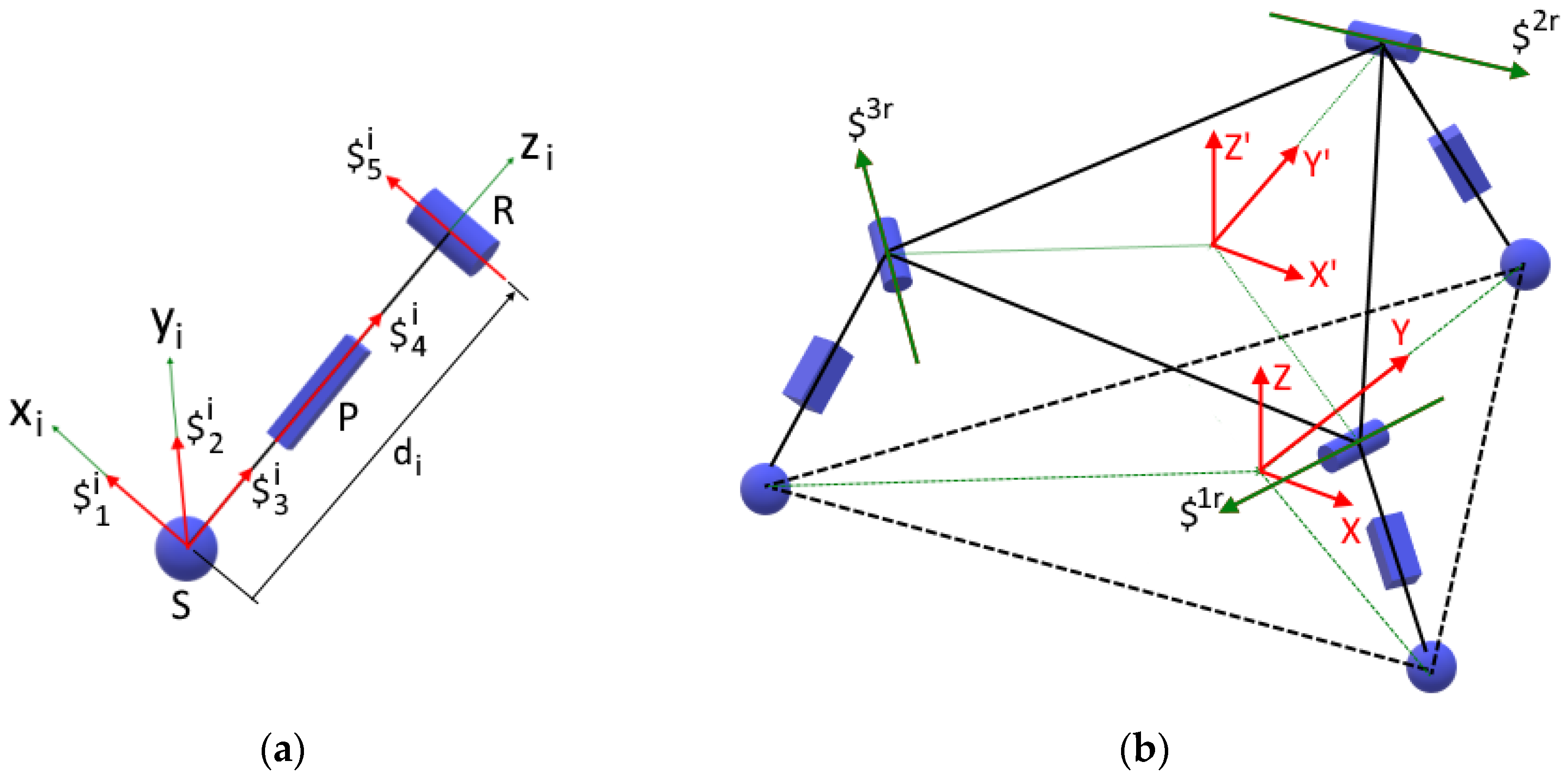
Referring to Figure 10a, the joint screws in the i-th limb of the 3SU mechanism can be written as follows:

$$\begin{gathered} {\$}^i={\left[{\$}_1^i {\$}_2^i {\$}_3^i {\$}_5^i {\$}_4^i\right]}^T\mathrm{for}\mathrm{the}\mathrm{first}\mathrm{configuration}\mathrm{of}\mathrm{the}\mathrm{U}\mathrm{joints}; \\ {\$}^i={\left[{\$}_1^i {\$}_2^i {\$}_3^i {\$}_4^i {\$}_5^i\right]}^T\mathrm{for}\mathrm{the}\sec \mathrm{ond}\mathrm{configuration}\mathrm{of}\mathrm{the}\mathrm{U}\mathrm{joints}, \end{gathered}$$

(3)

where the joint screws in their initial posture are given by the following:

$$\begin{gathered} {\$}_1^i=\left(1, 0, 0,0,0,0\right), \\ {\$}_2^i=\left(0, 1, 0,0,0,0\right), \\ {\$}_3^i=\left(0, 0, 1,0,0,0\right), \\ {\$}_4^i=\left(1, 0, 0,0,L,0\right), \\ {\$}_5^i=\left(0, 1, 0,-L,0, 0\right). \end{gathered}$$

(4)

These joint screws in both the U joint configurations create a 1-system in each limb. Accordingly, for both the U joint configurations, the reciprocal screw in the i-th limb is:

$${\$}^{ir}=(0,0,1,0,0,0)$$

(5)

which indicates a constraint force in the $z_i$ direction. In the initial posture, the three limbs of the 3SU mechanism have three constraint forces that are not coplanar and intersect at a common point, as depicted in Figure 10b. Therefore, the mechanism has three linearly independent constraint wrenches, namely three translations in the space. Accordingly, the freedom of the moving platform is 3R, that is, three rotations in the space. However, it turns out that this mobility is instantaneous and does not hold for the full-cycle motion of the mechanism. This is because the intersection at a point between the three constraint forces cannot be preserved in the full-cycle motion of the mechanism. Hence, after being displaced from its initial posture, the mobility of the 3SU mechanism turns from 3R to 1T2R, as presented in [22].

4. Pose Kinematics

4.1. Pose Kinematics of 3PRPR, 3PRRR, and Serial RR Mechanisms

The 3PRPR mechanism with the proximal P joints being actuated and the 3PRRR mechanism with the P joints being actuated have a unity mapping between the joint positions (x₁, x₂, and x₃) and end-effector position (x,y,z). In an actual implementation, there may be constant offsets between them. Since the kinematics of this mechanism is straightforward, it is not discussed in this paper.

The serial RR mechanism consists of a base, two R joints, and two links. The first link connects both the R joints, whereas the second link connects the last R joint with the tool center point (TCP). Since the pose kinematics of such a serial mechanism is well-known, it is not discussed here.

4.2. Pose Kinematics of 3SPR Mechanism

Figure 11 shows the 3SPR mechanism. Referring to the figure, the XYZ frame is fixed to the center of the mechanism base A, whereas the X′Y′Z′ frame is attached to the center of the moving platform. Both the base and the moving platform of the mechanism are equilateral triangles, namely A₁A₂A₃ and B₁B₂B₃, respectively. The circumradii of both triangles are, respectively, $R$ and $r$. The positions of the points A₁, A₂, and A₃ in the XYZ frame are given by the vectors ${\mathit{a}}_{\mathit{1}}$, ${\mathit{a}}_{\mathit{2}}$, and ${\mathit{a}}_{\mathit{3}}$, respectively, whereas the positions of the points B1, B2, and B3 in the X′Y′Z′ frame are given by the following vectors ${}_{}{}^{\mathit{P}}\mathit{b}{}_{\mathit{1}}$, ${}_{}{}^{\mathit{P}}\mathit{b}{}_{\mathit{2}}$, and ${}_{}{}^{\mathit{P}}\mathit{b}{}_{\mathit{3}}$, respectively.

The moving platform position and orientation are dictated by the lengths of the three active prismatic joints, namely $L_{1 }$, $L_{2 }$, and $L_{3 }$. The unit directional vectors of the active prismatic joints are ${\mathit{l}}_{\mathit{1}}$, ${\mathit{l}}_{\mathit{2}}$, and ${\mathit{l}}_{\mathit{3}}$, respectively. These unit vectors represent the orientation of the legs with respect to the XYZ frame. Since the 3PRPR mechanism already gives the spatial position, the used DOFs of the 3SPR mechanism are the spatial rotation defined by three Euler angles, namely ${\theta }_x$, ${\theta }_y$, and ${\theta }_z$_, which represent the rotation of the moving platform about the X, Y, and Z axes. However, as discussed in the mobility analysis, the rotation about the Z axis is coupled with translation.

Let vector $\mathit{p}$ denote the position of the center of the moving platform P with respect to point A. Let matrix ${\mathit{R}}_{\mathit{A}}^{\mathit{P}}$ be a rotation matrix representing the rotation of the moving platform, i.e., the moving frame X′Y′Z′, with respect to the base, i.e., the XYZ frame. The closed chain constraints of the 3SPR mechanism can be written in the following relation:

$$\mathit{p}-{\mathit{a}}_i-L_{i }{\mathit{l}}_{\mathit{i}}+{\mathit{R}}_{\mathit{A}}^{\mathit{P}} {}_{}{}^{\mathit{P}}\mathit{b}{}_{\mathit{i}}=0 \mathrm{where} i=1,2,3,$$

(6)

where the superscript P preceding a vector indicates that the vector is expressed in the X′Y′Z′ frame. A vector not preceded by any superscript is expressed in the XYZ frame.

The axes of the passive revolute joints are fixed to the moving platform. The orientation of these axes are defined by the unit directional vectors ${\mathit{w}}_{\mathit{1}}$, ${\mathit{w}}_{\mathit{2}}$, and ${\mathit{w}}_{\mathit{3}}$ which can be conveniently expressed in the X′Y′Z′ frame. The unit vectors ${\mathit{w}}_{\mathit{1}}$, ${\mathit{w}}_{\mathit{2}}$, and ${\mathit{w}}_{\mathit{3}}$ are always perpendicular to the vectors ${\mathit{b}}_{\mathit{1}}$, ${\mathit{b}}_{\mathit{2}}$, and ${\mathit{b}}_{\mathit{3}}$, respectively. Furthermore, each passive revolute joint constrains the motion of each leg I, i.e., the active prismatic joint, to be only a rotation about the axis of the passive revolute joint, while the leg changes its length $L_{i }$. Consequently, each leg is always perpendicular to the axis of the passive revolute joints. This perpendicularity constraint can be written as the following zero dot product:

$${\mathit{l}}_{\mathit{i}}{}^T{\mathit{R}}_{\mathit{A}}^{\mathit{P}} {}_{}{}^{\mathit{P}}\mathit{w}{}_{\mathit{i}}=0 \mathrm{where} i=1,2,3.$$

(7)

As both the vector b_i and leg l_i are always perpendicular to the axis of the passive revolute joint i, each limb creates a plane, namely AA_iB_iP. Consequently, the sum of the vectors p and b_i is also always perpendicular to the axis of the passive revolute joint ${\mathit{w}}_{\mathit{i}}$. This can be written as the following zero dot product:

$${\left(\mathit{p}+{\mathit{R}}_{\mathit{A}}^{\mathit{P}} {}_{}{}^{\mathit{P}}\mathit{b}{}_{\mathit{i}}\right)}^{\mathit{T}}{\mathit{R}}_{\mathit{A}}^{\mathit{P}} {}_{}{}^{\mathit{P}}\mathit{w}{}_{\mathit{i}}=0 \mathrm{where} i=1,2,3.$$

(8)

Equations (6)–(8) are the implicit kinematic equations of the 3SPR mechanism. The inverse kinematics problem can be stated as “given the orientation of the moving platform, find the corresponding active joint positions $L_{1 }$, $L_{2 }$, and $L_{3 }$”. Besides $L_{1 }$, $L_{2 }$, and $L_{3 }$, there are twelve other unknowns in the inverse kinematics problem, namely the unit directional vectors of the three legs (each of the unit vectors contains three components in X, Y, and Z directions) and the position of the moving platform (x,y,z). On the other hand, the forward kinematics problem can be stated as “given the active joint positions $L_{1 }$, $L_{2 }$, and $L_{3 }$, find the orientation of the moving platform”. Besides the three Euler angles of the moving platform, there are twelve other unknowns similar to those in the inverse kinematics problem.

4.3. Pose Kinematics of the 3SU Mechanism

Figure 12 shows the 3SU mechanism. Referring to the figure, the XYZ and X′Y′Z′ frames, similar to those in Section 4.2, are used. Similar to the 3SPR mechanism, the base is defined by the vectors ${\mathit{a}}_{\mathit{1}}$, ${\mathit{a}}_{\mathit{2}}$, and ${\mathit{a}}_{\mathit{3}}$ expressed in the XYZ frame, whereas the moving platform is defined by the vectors ${\mathit{b}}_{\mathit{1}}$, ${\mathit{b}}_{\mathit{2}}$, and ${\mathit{b}}_{\mathit{3}}$ expressed in the X′Y′Z′ frame. The unit directional vectors of the three legs are ${\mathit{l}}_{\mathit{1}}$, ${\mathit{l}}_{\mathit{2}}$, and ${\mathit{l}}_{\mathit{3}}$, respectively. These unit vectors represent the orientation of the legs with respect to the XYZ frame. All the legs have an identical, constant length L.

As discussed earlier, the 3SU mechanism can be implemented in two variations: the first variation in the 3SU mechanism, i.e., the 3SU mechanism with the first U joint configuration, and the second variation in the 3SU mechanism, i.e., the 3SU mechanism with the second U joint configuration. In the first variation, the R joints with the orientation given by the unit vectors ${\mathit{v}}_{\mathit{i}}$ are connected to the legs, whereas the R joints with the orientation given by the unit vectors ${\mathit{w}}_{\mathit{i}}$ are connected to the moving platform. In the second variation in the 3SU mechanism, the R joints with the orientation given by the unit vectors ${\mathit{v}}_{\mathit{i}}$ are connected to the moving platform, whereas the R joints with the orientation given by the unit vectors ${\mathit{w}}_{\mathit{i}}$ are connected to the legs. Hence, the unit vectors ${\mathit{w}}_{\mathit{1}}$, ${\mathit{w}}_{\mathit{2}}$, and ${\mathit{w}}_{\mathit{3}}$ in the second variation in the 3SU mechanism are always perpendicular to the unit directional vectors of the legs ${\mathit{l}}_{\mathit{1}}$, ${\mathit{l}}_{\mathit{2}}$, and ${\mathit{l}}_{\mathit{3}}$. This can be mathematically written as a zero dot product given in Equation (7), similar to the 3SPR mechanism. However, the lengths of the legs in the 3SU mechanism are fixed, whereas they are changed in the 3SPR mechanism. The first variation is actuated at the distal R joints, whereas the second is actuated at the intermediate R joints.

In each limb of both the variations, the axis ${\mathit{v}}_{\mathit{i}}$ is always perpendicular to the axis ${\mathit{w}}_{\mathit{i}}$, as both axes represent two R joints composing a U joint. This perpendicularity can be written as the following dot product:

$${\mathit{v}}_{\mathit{i}}{}^T{\mathit{R}}_{\mathit{A}}^{\mathit{P}}{}_{}{}^{\mathit{P}}\mathit{w}{}_{\mathit{i}}=0 \mathrm{where} i=1,2,3.$$

(9)

where the unit vector ${\mathit{v}}_{\mathit{i}}$ is defined in the XYZ frame, whereas the unit vector ${}_{}{}^{\mathit{P}}\mathit{w}{}_{\mathit{i}}$ is defined in the X′Y′Z′ frame.

The closed chain constraints of the first variation in the 3SU mechanism can be written in the following relation:

$$\mathit{p}+{\mathit{R}}_{\mathit{A}}^{\mathit{P}}{}_{}{}^{\mathit{P}}\mathit{b}{}_{\mathit{i}}-{\mathit{R}}_{\mathit{y}}\left({\theta }_{ai}\right){\mathit{R}}_{\mathit{x}}\left({\theta }_{pi}\right){}_{}{}^{B_i}\mathit{l}{}_{\mathit{i}}-{\mathit{a}}_{\mathit{i}}=0; i=1,2,3.$$

(10)

where the vector p denotes the position of the center of the moving platform P with respect to point A, whereas the matrix ${\mathit{R}}_{\mathit{A}}^{\mathit{P}}$ is a rotation matrix representing the rotation of the moving platform, i.e., the moving frame X′Y′Z′, with respect to the base, i.e., the XYZ frame. Since the R joints in each U joint rotate about the X and Y axes of a local frame which has the origin B_i and the Z direction aligned with the leg direction, the rotation of both the R joints can be represented by the rotation matrices ${\mathit{R}}_{\mathit{x}}$ and ${\mathit{R}}_{\mathit{y}}$ that, respectively, represent the elementary rotation matrices about the X and Y axes. The angles denote the magnitude of the rotations ${\theta }_{ai}$ and ${\theta }_{pi}$ that, respectively, denote the angles of the active and passive R joints of the U joint in the i-th limb. The vector ${}_{}{}^{{\mathit{B}}_{\mathit{i}}}\mathit{l}{}_{\mathit{i}}$ is the i-th leg vector expressed at its local frame that has the origin B_i, that is:

$${}_{}{}^{{\mathit{B}}_{\mathit{i}}}\mathit{l}{}_{\mathit{i}}={\left[\begin{array}{ccc}0& 0& 1\end{array}\right]}^T; i=1,2,3.$$

(11)

On the other hand, the closed chain constraints of the second variation in the 3SU mechanism can be written in the following relation:

$$\mathit{p}+{\mathit{R}}_{\mathit{A}}^{\mathit{P}}{}_{}{}^{\mathit{P}}\mathit{b}{}_{\mathit{i}}-{\mathit{R}}_{\mathit{x}}\left({\theta }_{pi}\right){\mathit{R}}_{\mathit{y}}\left({\theta }_{ai}\right){}_{}{}^{{\mathit{B}}_{\mathit{i}}}\mathit{l}{}_{\mathit{i}}-{\mathit{a}}_{\mathit{i}}=0; i=1,2,3.$$

(12)

The inverse kinematics problem can be stated as “given the orientation of the moving platform, find the corresponding active joint positions ${\theta }_{a1}$, ${\theta }_{a2}$, and ${\theta }_{a3}$”. Besides these active joint positions, there are six other unknowns in the inverse kinematics problem, namely the angles of the passive R joints of the i-th U joint (${\theta }_{p1}, {\theta }_{p2},{\theta }_{p3}$) and the position of the moving platform (x,y,z). On the other hand, the forward kinematics problem can be stated as “given the active joint positions${\theta }_{a1}$, ${\theta }_{a2}$, and ${\theta }_{a3}$, find the orientation of the moving platform”. Besides the three Euler angles of the moving platform, there are six other unknowns similar to those in the inverse kinematics problem.

4.4. Pose Kinematics of the Combined Mechanism

Figure 13 shows the combined 3SPR-3PRPR (or 3SPR-3PRRR) and 3SU-3PRPR (or 3SU-3PRRR) mechanisms consisting of the lower mechanisms serially connected with the pyramid structure of the upper 3PRPR or 3PRRR mechanism. The limbs of the 3PRPR or 3PRRR mechanism are not shown in the figure for more readability.

The XYZ frame is attached to the center of the base of the lower mechanism, namely, point A located in the world frame X_NY_NZ_N. In other words, the position of the whole mechanism in the world frame is given by the vector $\overrightarrow{\mathrm{NA}}$. This vector is constant when the whole mechanism is attached to the surface of the workpiece/structure, whereas the vector changes when the mechanism is walking. The X′Y′Z′ frame is attached to the moving platform of the 3SPR mechanism which serves as the base of the 3PRPR mechanism.

The pose of the end-effector of the 3PRPR or 3PRRR mechanism is conveniently expressed in the xyz frame. The intermediate X″Y″Z″ frame is defined to be used in conveniently formulating the kinematics of the walking motions of the mechanism and to conveniently transform from the xyz frame to the X′Y′Z′ frame. The Z′ and Z″ axes are always parallel with each other. There is no rotation between the X′Y′Z′ and X″Y″Z″ frames as both are attached to the same body, i.e., the moving platform of the 3SPR mechanism.

To express the position of the end-effector of the 3PRPR or 3PRRR mechanisms in the XYZ frame, first, the pose is defined in the xyz frame and, subsequently, transformed to the X″Y″Z″ frame, X′Y′Z′ frame, and, finally, to the XYZ frame. The orientation of the end-effector is identical to the orientation of the moving platform of the lower mechanism since the pyramid of the 3PRPR or 3PRRR mechanisms is axisymmetric. The pyramid has segments with an identical length L_p.

4.5. Numerical Example

A numerical simulation was conducted to implement the pose kinematics of the 6-DOF mechanisms utilizing the 3SPR and 3SU lower mechanisms. In this simulation, the circumradii of the lower mechanisms’ base and moving platform are R = 0.5 m and r = 0.4 m, respectively. In the 3SPR mechanism, the legs’ lengths are variable as they are the actuated P joints. In the 3SU mechanism, all the legs have an identical length of 0.3 m. The pyramid frame of the upper mechanism with 3PRPR topology has an angle of 90 degrees between its adjacent segments. Each segment has a length of 0.5 m. The upper mechanism is actuated at its proximal P joints.

In the inverse kinematics problem, the position of the end-effector E in both hybrid mechanisms was given to be coincident with the origin of X′Y′Z′ frame, namely point P. The orientation of the end-effector expressed as Euler angles with respect to the XYZ frame was given to be (0, 0, 0) in the 3SPR-3PRPR mechanism and (5, 0, 0) degrees in the 3SU-3PRPR mechanism. The forward kinematics of both the upper and lower mechanisms was solved by taking the solution of the inverse kinematics as the given actuator positions. The forward kinematics solution retrieved the end-effector pose given in the inverse kinematics problem. For each hybrid mechanism, the inverse and forward kinematics problems of the upper mechanism were solved analytically. In contrast, the lower mechanisms’ inverse and forward kinematics problems were solved numerically using the Levenberg–Marquardt algorithm in MATLAB.

The actuator positions and the end-effector poses obtained in the inverse and forward kinematics problems are shown in

Table 1. Actuator Positions and End-Effector Poses.

Mechanism	Actuator Position	End-Effector Pose
3SPR-3PRPR	$x_1$$=x_2$$=x_3$= 0.1667 m L1 = L2 = L3 = 0.3262 m	x = 0, y = 0, z = 0.3000 m ${\theta }_x$$={\theta }_y$$={\theta }_z$= 0
3SRꞱR-3PRPR	$x_1$$=x_2$$=x_3$= 0.1667 m ${\theta }_{a1}$$=-19.2743 \mathrm{deg}, {\theta }_{a2}$= 0, ${\theta }_{a3}$$=19.2743 \mathrm{deg}$	x = 0, y = 0.0948 m, z = 0.2651 m ${\theta }_x$$=5\mathrm{deg},{\theta }_y$$={\theta }_z$= 0
3SRꞱR-3PRPR	$x_1$$=x_2$$=x_3$= 0.1667 m ${\theta }_{a1}$$=-16.7787 \mathrm{deg}, {\theta }_{a2}$= 0, ${\theta }_{a3}$$=16.7786 \mathrm{deg}$	x = 0, y = 0.0948 m, z = 0.2651 m ${\theta }_x$$=5\mathrm{deg},{\theta }_y$$={\theta }_z$= 0

. The actuator positions of the upper mechanism, namely $x_1$, $x_2$, and $x_3$, are expressed in the xyz frame. The actuator positions of the 3SPR mechanism, namely L₁, L₂, and L_3, are expressed as constants representing the lengths of the actuated P joints. The actuator positions of both the variations in the SRꞱR (SU) mechanism, namely ${\theta }_{a1}$, ${\theta }_{a2}$, and ${\theta }_{a3}$, are expressed as constants representing the angles of the actuated R joints. The end-effector pose (x,y,z) and the end-effector orientation (${\theta }_x$, ${\theta }_y$, ${\theta }_z$) are expressed in the XYZ frame. Figure 14 and Figure 15, respectively, show the plots of the 3SPR-3PRPR and 3SU-3PRPR mechanisms in the XYZ frame.

5. Differential Kinematics and Singularity Analysis

In the differential kinematics formulation presented in this section, the Plucker coordinates of the joint screws refer to Figure 9 and Figure 10 used in Section 3, which discusses the mobility analysis.

5.1. Differential Kinematics and Singularity Analysis of 3PRPR and 3PRRR Mechanisms

With an orthogonal pyramid frame, the 3PRPR mechanism with the proximal P joints being actuated and the 3PRRR mechanism with the P joints being actuated have an identity 3 × 3 actuation Jacobian matrix. This implies a unity mapping between the twist of the moving platform and the twist of the actuators. When the intermediate P joints in the 3PRPR mechanism are actuated, it has a 3 × 3 actuation Jacobian matrix containing some trigonometric functions of the angles made by the intermediate P joint axes. The configuration singularities in both the 3PRPR and 3PRRR mechanisms only occur at their workspace boundary. Hence, they can be easily avoided. The 3PRPR and 3PRRR mechanisms have three constraint couples working on the moving platform that prevent the moving platform from rotating. Since these constraint couples are orthogonal, they never become dependent; hence, there is no constraint singularity in both mechanisms. Thus, there is no singularity inside the workspace of the 3PRPR and 3PRRR mechanisms.

5.2. Differential Kinematics and Singularity Analysis of 3SPR Mechanism

The instantaneous twist of the 3SPR moving platform is given by:

$${\$}_{\mathit{P}}={\dot{\theta }}_1^i{\widehat{\$}}_{\mathit{1}}^{\mathit{i}}+{\dot{\theta }}_2^i{\widehat{\$}}_{\mathit{2}}^{\mathit{i}}+{\dot{\theta }}_3^i{\widehat{\$}}_{\mathit{3}}^{\mathit{i}}+{\dot{d}}_i{\widehat{\$}}_{\mathit{4}}^{\mathit{i}}+{\dot{\theta }}_5^i{\widehat{\$}}_{\mathit{5}}^{\mathit{i}};i=1,2,3;$$

(13)

where ${\dot{\theta }}_1^i, {\dot{\theta }}_2^i, {\dot{\theta }}_3^i, {\dot{d}}_i,$and ${\dot{\theta }}_5^i$are the joint screws’ intensities, whereas the unit joint screws representing the five joints in the i-th limb are given by the following:

$${\widehat{\$}}_{\mathit{1}}^{\mathit{i}}=\left[\begin{array}{c}{\mathit{s}}_{\mathit{1}}^{\mathit{i}}\\ \left({\mathit{b}}_{\mathit{i}}-{\mathit{d}}_{\mathit{i}}\right)\times {\mathit{s}}_{\mathit{1}}^{\mathit{i}}\end{array}\right]$$

(14)

$${\widehat{\$}}_{\mathit{2}}^{\mathit{i}}=\left[\begin{array}{c}{\mathit{s}}_{\mathit{2}}^{\mathit{i}}\\ \left({\mathit{b}}_{\mathit{i}}-{\mathit{d}}_{\mathit{i}}\right)\times {\mathit{s}}_{\mathit{2}}^{\mathit{i}}\end{array}\right]$$

(15)

$${\widehat{\$}}_{\mathit{3}}^{\mathit{i}}=\left[\begin{array}{c}{\mathit{s}}_{\mathit{3}}^{\mathit{i}}\\ \left({\mathit{b}}_{\mathit{i}}-{\mathit{d}}_{\mathit{i}}\right)\times {\mathit{s}}_{\mathit{3}}^{\mathit{i}}\end{array}\right]$$

(16)

$${\widehat{\$}}_{\mathit{4}}^{\mathit{i}}=\left[\begin{array}{c}\mathit{0}\\ {\mathit{s}}_{\mathit{4}}^{\mathit{i}}\end{array}\right]$$

(17)

$${\widehat{\$}}_{\mathit{5}}^{\mathit{i}}=\left[\begin{array}{c}{\mathit{s}}_{\mathit{5}}^{\mathit{i}}\\ {\mathit{b}}_{\mathit{i}}\times {\mathit{s}}_{\mathit{5}}^{\mathit{i}}\end{array}\right]$$

(18)

Note that the vectors ${\mathit{b}}_{\mathit{i}}$ is expressed in the base frame, i.e., the XYZ frame, and accordingly can be written as:

$${\mathit{b}}_{\mathit{i}}={\mathit{R}}_{\mathit{A}}^{\mathit{P}}{}_{}{}^{\mathit{P}}\mathit{b}{}_{\mathit{i}}$$

(19)

where ${\mathit{R}}_{\mathit{A}}^{\mathit{P}}$ is the rotation matrix representing the rotation of the moving platform frame, i.e., the X′Y′Z′ frame, with respect to the base frame, whereas ${}_{}{}^{\mathit{P}}\mathit{b}{}_{\mathit{i}}$ is the vector $b_i$ expressed in the moving platform frame.

Since the axes of all the unactuated joints in each limb intersect the line passing A_i and B_i, a unique screw that is reciprocal to all the unactuated joint screws is:

$${\widehat{\$}}_{\mathit{4}}^{\mathit{i}\mathit{r}}=\left[\begin{array}{c}{\mathit{s}}_{\mathit{4}}^{\mathit{i}}\\ {\mathit{b}}_{\mathit{i}}\times {\mathit{s}}_{\mathit{4}}^{\mathit{i}}\end{array}\right]$$

(20)

Taking the reciprocal product of both sides of Equation (13) with Equation (20) yields the following relationship between the instantaneous twist of the moving platform ${\$}_{\mathit{P}}={\left[{\omega }_x {\omega }_y {\omega }_z \dot{x} \dot{y} \dot{z}\right]}^T$ and the instantaneous twist of the actuators $\dot{\mathit{q}}={\left[\begin{array}{ccc}{\dot{d}}_1& {\dot{d}}_2& {\dot{d}}_3\end{array}\right]}^T$:

$${\mathit{J}}_{\mathit{x}}{\$}_{\mathit{P}}={\mathit{J}}_{\mathit{q}}\dot{\mathit{q}}$$

(21)

where the forward Jacobian ${\mathit{J}}_{\mathit{x}}{}_{3x6}$ and the inverse Jacobian ${\mathit{J}}_{\mathit{q}}{}_{3x3}$ are given by:

$${\mathit{J}}_{\mathit{x}}=\left[\begin{array}{cc}{\left({\mathit{b}}_{\mathit{1}}\times {\mathit{s}}_{\mathit{4}}^{\mathit{1}}\right)}^T& {\left({\mathit{s}}_{\mathit{4}}^{\mathit{1}}\right)}^T\\ {\left({\mathit{b}}_{\mathit{2}}\times {\mathit{s}}_{\mathit{4}}^{\mathit{2}}\right)}^T& {\left({\mathit{s}}_{\mathit{4}}^{\mathit{2}}\right)}^T\\ {\left({\mathit{b}}_{\mathit{3}}\times {\mathit{s}}_{\mathit{4}}^{\mathit{3}}\right)}^T& {\left({\mathit{s}}_{\mathit{4}}^{\mathit{3}}\right)}^T\end{array}\right]$$

(22)

$${\mathit{J}}_{\mathit{q}}=\left[\begin{array}{ccc}{\mathit{s}}_{\mathit{4}}^{\mathit{1}}·{\mathit{e}}_{\mathit{1}}& 0& 0\\ 0& {\mathit{s}}_{\mathit{4}}^{\mathit{2}}·{\mathit{e}}_{\mathit{2}}& 0\\ 0& 0& {\mathit{s}}_{\mathit{4}}^{\mathit{3}}·{\mathit{e}}_{\mathit{3}}\end{array}\right]$$

(23)

The vectors denote the unit directional vectors of the actuation. In this case, ${\mathit{e}}_{\mathit{1}}={\mathit{s}}_{\mathit{4}}^{\mathit{1}}$, ${\mathit{e}}_{\mathit{2}}={\mathit{s}}_{\mathit{4}}^{\mathit{2}},$ and ${\mathit{e}}_{\mathit{3}}={\mathit{s}}_{\mathit{4}}^{\mathit{3}}$. Hence, ${\mathit{J}}_{\mathit{q}}$ is an identity matrix. The actuation Jacobian matrix ${\mathit{J}}_{\mathit{a}}{}_{3x6}$ is given by the following well-known equation:

$${\mathit{J}}_{\mathit{a}}={\mathit{J}}_{\mathit{q}}{}^{-1}{\mathit{J}}_{\mathit{x}}$$

(24)

On the other hand, taking the orthogonal product of both sides of Equation (13) with each of the reciprocal basis screws representing the constraint screws of the 3SPR mechanism yields the following relationship between the constraint Jacobian $J_c$ and the instantaneous twist of the moving platform ${\$}_{\mathit{P}}$:

$${\mathit{J}}_{\mathit{c}}{\$}_{\mathit{P}}=\mathit{0}$$

(25)

which indicates that the constraint wrenches perform no work on the moving platform. In the 3SPR mechanism, the constraint Jacobian $J_c{}_{3x6}$ is given by:

$${\mathit{J}}_{\mathit{c}}=\left[\begin{array}{cc}{\left({\mathit{b}}_{\mathit{1}}\times {\mathit{s}}_{\mathit{1}}^{\mathit{1}}\right)}^T& {\left({\mathit{s}}_{\mathit{1}}^{\mathit{1}}\right)}^T\\ {\left({\mathit{b}}_{\mathit{2}}\times {\mathit{s}}_{\mathit{1}}^{\mathit{2}}\right)}^T& {\left({\mathit{s}}_{\mathit{1}}^{\mathit{2}}\right)}^T\\ {\left({\mathit{b}}_{\mathit{3}}\times {\mathit{s}}_{\mathit{1}}^{\mathit{3}}\right)}^T& {\left({\mathit{s}}_{\mathit{1}}^{\mathit{3}}\right)}^T\end{array}\right]$$

(26)

As it is well-known, the overall Jacobian ${\mathit{J}}_{6\times 6}$is obtained by stacking the actuation Jacobian and the constraint Jacobian, that is:

$$\mathit{J}=\left[\begin{array}{c}{\mathit{J}}_{\mathit{a}}\\ {\mathit{J}}_{\mathit{c}}\end{array}\right]$$

(27)

The relationship between the overall Jacobian and the instantaneous twist of the moving platform is given by:

$$\mathit{J}{\$}_{\mathit{P}}={\dot{\mathit{q}}}_{\mathit{0}}$$

(28)

For the SPR mechanism, the vector ${\dot{q}}_0$ is given by:

$$\mathit{J}{\$}_{\mathit{P}}={\dot{\mathit{q}}}_{\mathit{0}}\mathrm{where}{\dot{\mathit{q}}}_{\mathit{0}}={\left[\begin{array}{ccc}{\dot{d}}_1& {\dot{d}}_2& {\dot{d}}_3\end{array} 0 0 0\right]}^T\mathrm{for}\mathrm{the}3\mathrm{SPR}\mathrm{mechanism}.$$

(29)

The architectural singularities occur in the 3SPR mechanism in three geometric conditions. First, an architectural singularity occurs if the three actuation forces lie on a common plane and intersect at one point. This happens when the moving platform collapses to the base. This singularity can be easily avoided by limiting the range of the S joints and adjusting the minimum limits of the P joints, namely L₁, L₂, and L₃, such that the moving platform cannot collapse to the base. Second, an architectural singularity occurs if the three actuation forces are parallel, as depicted in Figure 16a. This only occurs if the moving platform and the base have identical geometry and dimensions. Thus, this singularity can be easily avoided by making the moving platform smaller than the base. Third, an architectural singularity occurs if any of the P joint axes are collinear with the vector ${\mathit{b}}_{\mathit{i}}$ of the moving platform, as illustrated in Figure 16b.

The constraint singularity occurs when the three constraint forces, that are in the direction of the R joint axes, lie on a common plane and intersect at one point, as illustrated in Figure 16c. However, this geometrical condition is not the geometrical arrangement of the 3SPR mechanism at hand since the R joint axes are always perpendicular to the vector ${\mathit{b}}_{\mathit{i}}$. Hence, this constraint singularity never occurs.

5.3. Differential Kinematics and Singularity Analysis of 3SU Mechanism

The instantaneous twist of the 3SU moving platform is given by:

$${\$}_{\mathit{P}}={\dot{\theta }}_1^i{\widehat{\$}}_{\mathit{1}}^{\mathit{i}}+{\dot{\theta }}_2^i{\widehat{\$}}_{\mathit{2}}^{\mathit{i}}+{\dot{\theta }}_3^i{\widehat{\$}}_{\mathit{3}}^{\mathit{i}}+{\dot{\theta }}_4^i{\widehat{\$}}_{\mathit{4}}^{\mathit{i}}+{\dot{\theta }}_5^i{\widehat{\$}}_{\mathit{5}}^{\mathit{i}};i=1,2,3;$$

(30)

where ${\dot{\theta }}_1^i, {\dot{\theta }}_2^i, {\dot{\theta }}_3^i, {\dot{\theta }}_4^i,$and ${\dot{\theta }}_5^i$ are the joint screws’ intensities, whereas the unit joint screws of the i-th spherical joint, namely ${\widehat{\$}}_{\mathit{1}}^{\mathit{i}}$, ${\widehat{\$}}_{\mathit{2}}^{\mathit{i}}$, and ${\widehat{\$}}_{\mathit{3}}^{\mathit{i}}$, are identical to those in the 3SPR mechanism, i.e., Equations (14)–(16). The other unit joint screws corresponding to the i-th U joint are given by:

$${\widehat{\$}}_{\mathit{4}}^{\mathit{i}}=\left[\begin{array}{c}{\mathit{s}}_{\mathit{4}}^{\mathit{i}}\\ {\mathit{b}}_{\mathit{i}}\times {\mathit{s}}_{\mathit{4}}^{\mathit{i}}\end{array}\right]$$

(31)

$${\widehat{\$}}_{\mathit{5}}^{\mathit{i}}=\left[\begin{array}{c}{\mathit{s}}_{\mathit{5}}^{\mathit{i}}\\ {\mathit{b}}_{\mathit{i}}\times {\mathit{s}}_{\mathit{5}}^{\mathit{i}}\end{array}\right]$$

(32)

Note that the vectors ${\mathit{b}}_{\mathit{i}}$ are given by Equation (19).

When the R joints parallel with ${\mathit{w}}_{\mathit{1}}$, ${\mathit{w}}_{\mathit{2}}$, and ${\mathit{w}}_{\mathit{3}}$ axes are actuated, the instantaneous twist of the actuators is given by $\dot{\mathit{q}}={\left[\begin{array}{ccc}{\dot{\theta }}_4^1& {\dot{\theta }}_4^2& {\dot{\theta }}_4^3\end{array}\right]}^T$. On the other hand, when the R joints with ${\mathit{v}}_{\mathit{1}}$, ${\mathit{v}}_{\mathit{2}}$, and ${\mathit{v}}_{\mathit{3}}$ axes are actuated, the instantaneous twist of the actuators is given by $\dot{\mathit{q}}={\left[\begin{array}{ccc}{\dot{\theta }}_5^1& {\dot{\theta }}_5^2& {\dot{\theta }}_5^3\end{array}\right]}^T$. The forward Jacobian ${\mathit{J}}_x{}_{3\times 6}$ and the inverse Jacobian ${\mathit{J}}_{\mathit{q}}{}_{3\times 3}$ are given by:

$${\mathit{J}}_{\mathit{x}}=\left[\begin{array}{cc}{\left({\mathit{b}}_{\mathit{1}}\times {\mathit{s}}_{\mathit{3}}^{\mathit{1}}\right)}^T& {\left({\mathit{s}}_{\mathit{3}}^{\mathit{1}}\right)}^T\\ {\left({\mathit{b}}_{\mathit{2}}\times {\mathit{s}}_{\mathit{3}}^{\mathit{2}}\right)}^T& {\left({\mathit{s}}_{\mathit{3}}^{\mathit{2}}\right)}^T\\ {\left({\mathit{b}}_{\mathit{3}}\times {\mathit{s}}_{\mathit{3}}^{\mathit{3}}\right)}^T& {\left({\mathit{s}}_{\mathit{3}}^{\mathit{3}}\right)}^T\end{array}\right]$$

(33)

$$J_q=\left[\begin{array}{ccc}{\mathit{s}}_{\mathit{3}}^{\mathit{1}}·{\mathit{e}}_{\mathit{1}}& 0& 0\\ 0& {\mathit{s}}_{\mathit{3}}^{\mathit{2}}·{\mathit{e}}_{\mathit{2}}& 0\\ 0& 0& {\mathit{s}}_{\mathit{3}}^{\mathit{3}}·{\mathit{e}}_{\mathit{3}}\end{array}\right]$$

(34)

The vectors denote the unit directional vectors of the actuation. If the R joints parallel with the unit vectors ${\mathit{w}}_{\mathit{1}}$, ${\mathit{w}}_{\mathit{2}}$, and ${\mathit{w}}_{\mathit{3}}$ are actuated, ${\mathit{e}}_{\mathit{1}}={\mathit{s}}_{\mathit{4}}^{\mathit{1}}$, ${\mathit{e}}_{\mathit{2}}={\mathit{s}}_{\mathit{4}}^{\mathit{2}},$ and ${\mathit{e}}_{\mathit{3}}={\mathit{s}}_{\mathit{4}}^{\mathit{3}}$. On the other hand, if the R joints parallel with the unit vectors ${\mathit{v}}_{\mathit{1}}$, ${\mathit{v}}_{\mathit{2}}$, and ${\mathit{v}}_{\mathit{3}}$ are actuated, ${\mathit{e}}_{\mathit{1}}={\mathit{s}}_{\mathit{5}}^{\mathit{1}}$, ${\mathit{e}}_{\mathit{2}}={\mathit{s}}_{\mathit{5}}^{\mathit{2}},$ and ${\mathit{e}}_{\mathit{3}}={\mathit{s}}_{\mathit{5}}^{\mathit{3}}$. The actuation Jacobian matrix ${\mathit{J}}_{\mathit{a}}{}_{3x6}$ is given by Equation (24).

The constraint Jacobian ${\mathit{J}}_{\mathit{c}}{}_{3x6}$ is given by:

$${\mathit{J}}_{\mathit{c}}=\left[\begin{array}{cc}{\left({\mathit{b}}_{\mathit{1}}\times {\mathit{s}}_{\mathit{3}}^{\mathit{1}}\right)}^T& {\left({\mathit{s}}_{\mathit{3}}^{\mathit{1}}\right)}^T\\ {\left({\mathit{b}}_{\mathit{2}}\times {\mathit{s}}_{\mathit{3}}^{\mathit{2}}\right)}^T& {\left({\mathit{s}}_{\mathit{3}}^{\mathit{2}}\right)}^T\\ {\left({\mathit{b}}_{\mathit{3}}\times {\mathit{s}}_{\mathit{3}}^{\mathit{3}}\right)}^T& {\left({\mathit{s}}_{\mathit{3}}^{\mathit{3}}\right)}^T\end{array}\right]$$

(35)

The overall Jacobian ${\mathit{J}}_{6\times 6}$is given by Equation (27), whereas the relationship between the overall Jacobian and the instantaneous twist of the moving platform is given by Equation (28).

The 3SU mechanism undergoes an architectural singularity in two geometric conditions. First, the architectural singularity occurs if the unit vectors ${\mathit{v}}_{\mathit{1}}$, ${\mathit{v}}_{\mathit{2}}$, and ${\mathit{v}}_{\mathit{3}}$ lie on a common plane and intersect at one point. The latter condition occurs all the time, but the former only occurs in the architectural singularity. This singularity happens when the moving platform collapses to the base or when the three links are parallel, as illustrated in Figure 16d. As in the 3SPR mechanism, the collapse of the moving platform to the base can be easily avoided by limiting the range of the S joints and making the link length L long enough. The parallelism of the three links only occurs when the moving platform and the base have identical geometry and dimensions. This can be easily avoided by making the moving platform smaller than the base. The second geometric condition leading to an architectural singularity is a condition in which the unit vectors ${\mathit{w}}_{\mathit{1}}$, ${\mathit{w}}_{\mathit{2}}$, and ${\mathit{w}}_{\mathit{3}}$ lie on a common plane and intersect at one point. The former condition occurs at all times, but the latter condition never occurs since the unit vectors ${\mathit{w}}_{\mathit{1}}$, ${\mathit{w}}_{\mathit{2}}$, and ${\mathit{w}}_{\mathit{3}}$ are always perpendicular to the vectors ${\mathit{b}}_{\mathit{i}}$.

The constraint singularity occurs in the 3SU mechanism if the three constraint forces lie on a common plane or are parallel. The former condition occurs when the moving platform collapses to the base. The latter condition occurs when the three links of the mechanism are parallel to each other, i.e., when the moving platform and the base have identical geometry and dimensions. Thus, the constraint singularity can be avoided easily.

6. Workspace

6.1. Workspace of the 3T Mechanism

With a pyramid frame having an angle of 90 degrees between its adjacent segments, the upper mechanism, i.e., the 3PRPR or 3PRRR mechanism, has a rectangular cuboid workspace with a size mainly dictated by the motion limits of the actuators, as illustrated in Figure 17a.

6.2. Workspace of the Serial RR Mechanism

The serial RR mechanism in the 3T2R mechanism has a large orientation workspace, mainly limited by the collision among the mechanical components, cabling, and motors’ rotation limits. In the serial RR mechanism, as depicted in Figure 17b, its orientation is coupled with dependent translation due to the non-zero distance between both the R joints’ axes and the non-zero distance between the TCP and the axis of the last R joint. In this case, the dependent translation should be compensated by translating the 3T mechanism. The serial RR mechanism’s total orientation workspace is shown in Figure 17c, given the R joints’ tilting range between −90 and 90 degrees. The orientation workspace in the 3T robot combined with the serial RR module is identical across the position workspace of the 3T robot unless there is a collision around the boundary of the position workspace that may reduce the actual tilting capability of the serial RR module.

6.3. Workspace of the 3SPR and 3SU Mechanisms

The 3SPR and 3SU mechanisms have a more limited orientation workspace. However, their parallel kinematics are expected to provide higher stiffness than the serial RR mechanism. Considering this, a five-axis machining task that typically requires a large orientation workspace is more convenient to perform using the 3T2R mechanism while the overall stiffness is compromised. On the other hand, the 6-DOF mechanisms are more appropriate for machining workpiece/structure with an irregular surface while higher stiffness is prioritized.

The workspace of the 3SPR mechanism can be determined graphically by first finding the intersection of three hollow spheres created by the three SP chains of the mechanism. To determine a constant orientation workspace, the reachable points previously obtained need to be shifted to the center of the moving platform at a specific orientation. To determine the total orientation workspace, the moving platform is rotated about the three R joints to create the outer layer of the workspace. The limits of the S, P, and R joints also dictate the reachable workspace. Figure 18a,b shows the total orientation workspaces of 3SPR mechanisms with two different sizes of the fixed base.

The workspace of the 3SU mechanism can be determined graphically by first finding the centers of rotation of the U joints, that is, lying on three spherical surfaces created by the tips of the three links of the mechanism. Subsequently, assuming that both the R joints in each U joint have axes intersecting at a point, the constant orientation workspace can be created by shifting the previously obtained reachable points to the center of the moving platform at a specific orientation. In contrast, the total orientation workspace is obtained by rotating both the R joints of each U joint about the known centers of rotation lying on the previously created surface. The limits of the S and U joints in all three limbs also affect the workspace. Figure 18c shows the total orientation workspace of a 3SU mechanism.

When a 3SPR or 3SU mechanism is combined with the 3T mechanism, the workspace of the combined robot is a superposition of the workspace of the 3SPR or 3SU mechanism and the workspace of the 3T mechanism. The workspace of the 3SPR or 3SU mechanism combined with the 3T mechanism is the rectangular cuboid of the 3T mechanism being tilted by the 3SPR or 3SU mechanism. However, it is not a purely tilting motion due to the dependent translational motion in the 3SPR or 3SU mechanism. Since the 3T mechanism does not have any rotational DOF, it only contributes to the translational components. Since the 3SPR or 3SU mechanism has dependent translational motion, its translation should be added to the translation of the 3T mechanism to obtain the combined translation.

7. Reconfiguration Schemes

Modularity and joint locking can be used to achieve reconfigurability. In the modularity scheme, two possible scenarios can be implemented, as illustrated in Figure 18. With the 3T mechanism as the basic build, modular components can be added to make a 3-DOF, 5-DOF, or 6-DOF robot. In Figure 19a, the attachment pad and spherical joint are included in each module. This requires less time for assembly but requires more attachment pads and spherical joints. In Figure 19b, the attachment pad and spherical joint are made as separate modules, namely AS modules. Accordingly, the same set of AS modules can be used with various modules such as serial RR, PR, and SU modules. This requires a lower number of AS modules but requires more time for assembly. For both the modularity scenarios, the design of interfaces between mating parts should be made to enable the self-alignment of the mating parts. If required, a calibration routine can be run after an assembly to increase the robot’s accuracy.

It is not always necessary to have all the modules. One only needs certain modules based on the need. For three-axis machining, only the modules for the 3-DOF robot are needed. For five-axis machining, only the modules for the 5-DOF robot are needed. For six-axis machining, either the modules for the 3SPR or SU mechanism are needed. If a capability to switch between three-axis and five-axis machining or between three-axis and six-axis machining is required, one only needs the required modules.

In the joint locking scheme, reassembly is not required since a module is always assembled. One can simply lock some joints for specific mobility to change the robot’s DOF. A switch between three-axis and five-axis machining can be performed by using lockable serial RR mechanism, as illustrated in Figure 20a. Since both the R joints in the serial RR mechanism are actuated, locking both the R joints to change the robot to a 3T mobility can be simply achieved by locking the R joints’ actuators. A switch from a six-axis robot with a 3SPR mechanism to a 3T robot can be performed by locking the active P joints and the passive R joint. As depicted in Figure 20b, locking the active P joints can be performed by simply locking their actuators, whereas locking the passive R joints can be achieved by using a certain design of a lockable passive R joint. A switch from a six-axis robot with a 3SU mechanism to a 3T robot can be performed by locking the actuated R joints and the passive R joints. As illustrated in Figure 20c,d, locking the actuated R joints can be simply achieved by locking their actuator, whereas locking the passive R joints can be achieved by using a certain design of a lockable passive R joint. The design of lockable passive R joints is beyond the scope of this paper.

8. Dimensional Optimization

It is widely known that the main drawback of parallel mechanisms is their limited workspace. In this section, we discuss a method to optimize some dimensions of the proposed mechanisms to obtain the optimal workspace.

8.1. Optimization of the 3T Mechanism

Since the motion limits of the actuators mainly dictate the workspace of the 3T mechanism, its volume can be easily maximized by increasing the length of the pyramid segments such that its linear actuators have a longer sliding span. Since this implies increasing the size of the mechanism, one may compromise it with its resulting footprint and weight. Since this optimization is straightforward, it is not discussed in detail here.

8.2. Optimization of the Serial RR Mechanism

The serial RR mechanism theoretically can make a full rotation about its two R joints’ axes. However, due to cabling and collision among components, the tilting limits of the mechanism in the real practice are typically between −90 and 90 degrees. In general, this range is sufficient to perform any five-axis machining. To minimize the translational compensation that the 3T mechanism should provide due to the dependent translation of the serial RR mechanism, it is preferred to minimize the length of the two links in the serial RR mechanism as far as possible.

8.3. Optimization of the 3SPR and 3SU Mechanisms

8.3.1. Design Variables

Since the translational workspace of the 3SPR and 3SU mechanisms are provided by the intersection between the workspaces of each limb, the volume of the intersection is dictated by the position of the three S joints of each mechanism, that is defined by the circumradius of the base, $\left|{\mathit{a}}_{\mathit{i}}\right|$. The total orientation workspace is affected by the size of the moving platform, that is defined by its circumradius, $\left|{\mathit{b}}_{\mathit{i}}\right|$. Therefore, both $\left|{\mathit{a}}_{\mathit{i}}\right|$ and $\left|{\mathit{b}}_{\mathit{i}}\right|$ are considered the design variables in the optimization of the 3SPR ad 3SU mechanisms. In the 3SPR mechanism, the volume of the intersection is also dictated by the range of the active P joints, that is the span between their lower and upper limits, namely $L_i,min$ and $L_i,max$. It is quite intuitive to say that the larger the range of the active P joints, the higher the tilting capability of the 3SPR mechanism. Accordingly, maximizing the tilting capability of the 3SPR mechanism can be performed by simply enlarging the range of their active P joints. Since this is trivial,$L_i,min$ and $L_i,max$ are not included as the design va-riables in the optimization of the 3SPR mechanism. Instead, they are determined a priori based on the design consideration. On the other hand, in the 3SU mechanism, the volume intersection is also dictated by the link length, $L_i$. This parameter is considered a design variable in the optimization of the 3SU mechanism. All the mentioned design parameters are to be optimized to obtain an optimal workspace.

8.3.2. Optimization Constraints

The optimization constraints consist of design, technological, and interference constraints. The design constraints are the constraints that involve the design variables. Assuming that the base and the moving platform have equidistant triangles, $\left|{\mathit{a}}_{\mathit{1}}\right|=\left|{\mathit{a}}_{\mathit{2}}\right|=\left|{\mathit{a}}_{\mathit{3}}\right|=R$ and $\left|{\mathit{b}}_{\mathit{1}}\right|=\left|{\mathit{b}}_{\mathit{2}}\right|=\left|{\mathit{b}}_{\mathit{3}}\right|=r$. For design consideration, we can determine the lower and upper bounds of R and r, which can be written as:

$$\begin{gathered} R_{min} \le R \le R_{max} \\ {r}_{min} \le r \le r_{max} \end{gathered}$$

(36)

For the 3SU mechanism, the lower and upper bounds of the link length $L_i$ can be written as:

$$L_{i,min} \le L_i \le L_{i,max}$$

(37)

The base circumradius should not be equal to the moving platform circumradius to avoid singularity, as discussed earlier. For better stability of the mechanism, let us constraint the base circumradius to be larger than the moving platform circumradius. This can be written as the following inequality:

$$-R+r \le 0$$

(38)

The technological constraints do not involve the design variables. They are determined based on the technological limitations of some components of the mechanism. In this case, the limits of the S, R, and U joints are the technological constraints of the optimization. In fact, these joints’ limits also affect the workspace.

The interference constraints are the constraints determined to avoid collision bet-ween the mechanism components. In this case, we constraint the mechanism to avoid collision between the moving platform and the base. Considering that the moving platform with the circumradius $r$ can tilt at angles ${\theta }_x$ and ${\theta }_y$ about the X and Y axes, respectively, this can be written as the following inequality constraints:

$$\left|r\sin {\theta }_x\right|-z<0$$

(39)

$$\left|r\sin {\theta }_y\right|-z<0$$

(40)

The constraints in Equations (39) and (40) also avoid the mechanism from its singular configuration associated with the collapse of the moving platform to the base.

8.3.3. Objective Function

Since the 3SPR and 3SU mechanisms’ main purpose is to provide tilting capability, the objective of the workspace optimization should be to maximize the orientation workspace. Since the orientation workspace is defined by the moving platform angles θ_x and θ_y, maximizing the range of each angle can be written as maximizing the difference between the maximum and minimum limits of each angle, i.e., ${\theta }_{x,max}-{\theta }_{x,min}$ and ${\theta }_{y,max}-{\theta }_{y,min}$_. Since there are two ranges of angles to be maximized, it is more practical in the optimization algorithm to combine both as a single objective given by the sum of them. Hence, the single objective function can be written as the following weighted sum:

$$f_{maximization}=g_1\left({\theta }_{x,max}-{\theta }_{x,min}\right)+g_2\left({\theta }_{y,max}-{\theta }_{y,min}\right)$$

(41)

where $g_1$ and $g_2$ denote the weights of both terms in the right hand side of Equation (41). Since the ranges of both the angles ${\theta }_x$ and ${\theta }_y$ are equally important, we use $g_1=g_2=1.$

If the optimization is written as a minimization problem, the constrained optimization formulation is to minimize the negative of the aforementioned objective function, i.e.:

$$f_{minimization}=-f_{maximization}$$

(42)

8.3.4. Optimization Formulation

The workspace optimization problem can be formulated as a constrained optimization problem. Accordingly, the workspace optimization of the 3SPR mechanism can be stated as follows:

Find the optimum design parameters $R$ and $r$

that maximize the objective function $f_{maximization}$ given in Equation (41)

subject to:

• the lower and upper bounds of $R$ as written in Equation (36);
• the lower and upper bounds of $r$ as written in Equation (36);
• the inequality constraint written in Equation (38);
• the limits of the S joints, i.e., ${\theta }_{pj,min}^{is}\le {\theta }_{pj}^{is}\le {\theta }_{pj,max}^{is}$ for i = 1,2,3 and j = 1,2,3;
• the limits of the R joints, i.e., ${\theta }_{pi,min}\le {\theta }_{pi}\le {\theta }_{pi,max}$ for i = 1,2,3;
• the interference constraints written in Equations (39) and (40).

On the other hand, the workspace optimization of the 3SU mechanism can be stated as follows:

Find the optimum design parameters$R$,$r,$ and $L_i$

that maximize the objective function $f_{maximization}$ given in Equation (48)

subject to:

• the lower and upper bounds of $R$ as written in Equation (36);
• the lower and upper bounds of $r$ as written in Equation (36);
• the lower and upper bounds of $L_i$ as written in Equation (37);
• the inequality constraint written in Equation (38);
• the limits of the S joints, i.e., ${\theta }_{pj,min}^i\le {\theta }_{pj}^i\le {\theta }_{pj,max}^i$ for i = 1,2,3 and j = 1,2,3;
• the limits of the U joints, i.e., ${\theta }_{ai,min}\le {\theta }_{ai}\le {\theta }_{ai,max}$ and ${\theta }_{pi,min}\le {\theta }_{pi}\le {\theta }_{pi,max}$ for i = 1,2,3;
• the interference constraints written in Equations (39) and (40).

8.3.5. Optimization Algorithm

The objective function is computed using the following routine:

• Step 1: Run the forward kinematics of the mechanism by inputting the active joints’ positions at a specific discretization interval within their ranges. The tilting angles of the moving platform ${\theta }_x$ and ${\theta }_y$ corresponding to the input active joints’ positions are obtained from the forward kinematics solution. It is worth mentioning that the lower and upper limits of the active P joints, $L_{i,min}$ and $L_{i,max}$, determined a priori in the 3SPR mechanism, can be considered pre-determined constraints that are not part of the optimization. Similarly, the limits of the active joints in the 3SU mechanism that are determined a priori can also be considered pre-determined constraints that are not part of the optimization.
• Step 2: Extract the minimum and maximum values of the obtained tilting angles of the moving platform ${\theta }_x$ and ${\theta }_y$. This gives us ${\theta }_{x,min}$, ${\theta }_{x,max}$, ${\theta }_{y,min}$, and ${\theta }_{y,max}$.
• Step 3: Compute the objective function written in Equations (41) or (42), depending on whether it is maximization or minimization.

The constrained optimization problem formulated above was solved by using genetic algorithm optimizer, namely ga, in MATLAB. It is a global optimizer that can avoid getting trapped in a local optimum.

8.3.6. Numerical Example

Here, we present an example of the optimization of the 3SPR and 3SU mechanisms. As described earlier, the design variables in the optimization of the 3SPR mechanism are R and $r$, whereas the design variables in the optimization of the 3SU mechanism are R, r, and $L_i$ The lower and upper bounds of the design variables are $0.3\mathrm{m}\le R\le 0.6\mathrm{m}$, $0.2\mathrm{m}\le r\le 0.5\mathrm{m}$, and $0.2\mathrm{m}\le L_i\le 0.6\mathrm{m}$. The inequality constraints written in Equations (38)–(40) are imposed. The lower and upper rotational limits of the S, R, and U joints are −70 deg and 70 deg, unless specified otherwise.

The forward kinematics of the 3SPR and 3SU mechanisms were solved by iterating the active joints positions from their minimum values to their maximum values at a certain discretization interval. The smaller the interval, the finer the visualization of the mechanism workspace, but the longer the time required for the optimization, and vice versa. In the optimization, the parameters of the genetic algorithm optimizer are shown in

Table 2. Parameters of the MATLAB genetic algorithm optimizer.

Parameter	Value
Population size	50
Maximum generations	$100$ the number of design variables
Creation function	Random initial population satisfying bounds and linear constraints
Mutation function	Mutation Adapt Feasible
Selection function	Stochastic Uniform
Crossover function	CrossoverIntermediate (weighted average of the parents)
Crossover fraction	0.8
Elite count	3
Function tolerance	$1\times {10}^{-6}$
Constraint tolerance	$1\times {10}^{-3}$
Maximum stall generations	50
Maximum stall time	$\infty$
Maximum time	$\infty$

.

Using a computer having 3 GHz Intel^® Xeon^® processor and 64 GB RAM, the optimization of the 3SPR with forward kinematics discretization interval of 0.01 m took 340 min. On the other hand, the optimization of the 3SU mechanisms with the forward kinematics discretization interval of 0.01 deg took 1125 min. The optimization stopped after the average change in the fitness value is less than the function tolerance. The optimization of the 3SPR mechanism gives the following optimized design variables: R = 0.549 m and r = 0.205 m. On the other hand, the optimization of the 3SU mechanism gives the following optimized design variables: R = 0.533 m, r = 0.234 m, and $L_1=L_2=L_3=$ 0.493 m.

Figure 21 shows the orientation workspace of the optimized 3SPR mechanism in multiple views. The discretization interval of 0.01 m, which is considered quite large, does not provide a smooth boundary of the workspace visualization. It is shown that the optimized 3SPR mechanism can be tilted from approximately −25 deg to 12.5 deg about the X axis and from approximately −20 deg to 20 deg about the Y axis. The dots in the figure, regardless of their color, represent the reachable tilting angles in the 3SPR mechanism. It can be seen in Figure 21b that the tilting range about the Y axis is symmetric. This is because the mechanism is symmetric with respect to the Y axis. In contrast, the tilting range about the X axis is larger in the negative direction than in the positive direction as the mechanism is not symmetric with respect to the X axis. The moving platform can be tilted more to a negative angle about the X axis since this tilting requires only one link to be lowered. On the other hand, the moving platform can be tilted less to a positive angle about the X axis since this tilting requires two links to be lowered. Figure 22 shows some postures of the tilted 3SPR mechanism.

In a similar fashion, Figure 23 shows in multiple views the orientation workspace of the optimized 3SU mechanism given the lower and upper limits of the S and U joints of −80 deg and 80 deg. The discretization interval of 0.01 deg, which is considered quite small, provides a smooth boundary of the workspace visualization. It is shown that the optimized 3SPR mechanism can be tilted from approximately −80 deg to 60 deg about the X axis and from approximately −40 deg to 40 deg about the Y axis. The dots in the figure, regardless of their color, represent the reachable tilting angles in the 3SU mechanism. The symmetry of the tilting range about the Y axis and the non-symmetry of the tilting range about the X axis have a similar reason to the case in the 3SPR mechanism. Furthermore, it is quite intuitive to say that longer links in the SU mechanism lead to larger tilting angles since the moving platform can be tilted at a larger angle without colliding with the base. Figure 24 shows some postures of the tilted 3SU mechanism.

However, when the rotational ranges of the S and U joints are tightened, the orientational workspace of the 3SU mechanism becomes smaller. The tighter the ranges of the S and U joints, the smaller the orientation workspace. For example, when the lower and upper limits of the S and U joints are changed to −30 deg and 30 deg, the orientation workspace of the 3SU mechanism is shrunk to that shown in Figure 25. It is clear that this smaller orientation workspace is a subset of the larger one shown in Figure 23. It is shown in the figure that the optimized 3SPR mechanism can be tilted from approximately –30 deg to 17.5 deg about the X axis and from approximately −15 deg to 15 deg about the Y axis. Figure 26 shows some postures of the tilted 3SU mechanism.

Comparing the orientation workspace of the 3SPR and 3SU joints, we observed that tilting capability of the 3SPR mechanism is much dictated by the range of the active P joints’ motion besides the ranges of the S and R joints. The 3SPR mechanism provides a larger tilting angle when one of links is shortened to its minimum while the other links are lengthened to their maximum, or when two links are shortened to their minimum while the other link is lengthened to its maximum. On the other hand, the orientation workspace of the 3SU mechanism is mainly limited by the rotational range of the S and U joints. Although the 3SU mechanism theoretically has a quite large orientation workspace, the technological limitation of the S and U joints typically provides a quite tight rotational ranges.

9. Design Considerations

Although parallel mechanisms in general are theoretically more rigid than serial mechanisms due to their closed chains, the number of joints in the parallel mechanisms is typically larger than those in serial mechanisms. This is often believed to be among the reasons why the parallel mechanisms in general often cannot outperform well-designed and well-manufactured serial mechanisms, particularly the Cartesian/gantry serial machines. Nevertheless, compared to articulated serial robots, well-designed and well-manufactured parallel robots are typically more rigid, despite their more limited workspace. Hence, the proposed parallel robot is to compete with the articulated serial robots, not the Cartesian/gantry machines. For the machining of large structures, the use of Cartesian/gantry machines are often not feasible as the use of such machines requires the structures/workpieces to be inserted within the machines’ volume. Hence, in such scenarios, the articulated serial robots are currently often used. Such robots suffer a lot from low rigidity when it is significantly extended, unless the robots are built with bulky and heavy arms. The size and weight of on-structure (adsorption) parallel robots, such as the one proposed in this paper, are much lower with comparable and even better stiffness. The high stiffness is due to two reasons: (1) the closed chain of the parallel mechanisms, and (2) the direct attachment of the mechanism to the structure/workpiece.

To overcome possible low accuracy and stiffness due to the presence of many joints in parallel mechanisms, one should have a good detail design and engineering practice to physically implement the joints, for example, by using preloaded bearings and precision bearings with good assembly fit and tolerance. When the joint locking scheme is used for the reconfiguration, the lockable joints should be designed carefully to avoid significant clearance or backlash that may deteriorate the robot performance. Finally, the manufacturing and assembly of the robot links should be performed with appropriate fit and to-lerance to avoid the resulting inaccuracy due to manufacturing and assembly errors.

10. Conclusions

A novel modular/reconfigurable walking robot topology with 3T2R manipulation capability, namely, 3A+3S+3PRPR+1RR (or 3A+3S+3PRRR+1RR), and two novel modular/reconfigurable walking robots with six-DOF manipulation capability, namely, 3A+3SPR+3PRPR (or 3A+3SPR+3PRRR) and 3A+3SRꞱR(3SU)+3PRPR (or 3A+3SRꞱR(3SU)+3PRRR), are proposed. Furthermore, the 3A+3SRꞱR(3SU)+3PRPR (or 3A+3SRꞱR(3SU)+3PRRR) topology is presented in two variations. The 3T module of all the robot topologies is a 3PRPR or 3PRRR parallel mechanism. Attachment pads are serially connected with S joints to the base frames of the hybrid-kinematics mechanisms, while a support is attached to the moving platform of the mechanisms. It was shown that the 3T robot can be reconfigured to a 3T2R or six-DOF robot capable of adjusting the orientation of its tool to be perpendicular to the irregular surface of a workpiece/structure and capable of performing five- or six-axis machining tasks. This reconfiguration can be performed by either reassembly or joint locking. It was shown that the 3T2R robot utilizing a serial RR module to provide the rotational DOFs has larger orientation workspace compared to the six-DOF robots utilizing the 3SPR and 3SU modules. Therefore, the 3T2R robot is more appropriate to be used in a five-axis machining task due to its larger orientation workspace, whereas the six-DOF robots are appropriate to be used for applications that require an angular adjustment due to an irregular or uneven surface of large workpieces/structures.

11. Patent

The content of this paper is a part of the authors’ pending patent application US 63/184.505 entitled “Reconfigurable Walking Robot”.

References

1. Axinte, D.A.; Allen, J.M.; Anderson, R.; Dane, I.; Uriarte, L.; Olara, A. Free-leg Hexapod: A novel approach of using parallel kinematic platforms for developing miniature machine tools for special purpose operations. CIRP Ann. 2011, 60, 395–398. [Google Scholar] [CrossRef]
2. Rushworth, A.; Cobos-Guzman, S.; Axinte, D.A.; Raffles, M. Pre-gait analysis using optimal parameters for a walking machine tool based on a free-leg hexapod structure. Robot. Auton. Syst. 2015, 70, 36–51. [Google Scholar] [CrossRef] [Green Version]
3. Olarra, A.; Axinte, D.; Uriarte, L.; Bueno, R. Machining with the WalkingHex: A walking parallel kinematic machine tool for in situ operations. CIRP Ann. 2017, 66, 361–364. [Google Scholar] [CrossRef]
4. Chen, J.; Xie, F.; Liu, X.; Bi, W. Stiffness Evaluation of an Adsorption Robot for Large-Scale Structural Parts Processing. ASME J. Mech. Robot. 2021, 13, 040902. [Google Scholar] [CrossRef]
5. Tedeschi, F.; Carbone, G. Design Issues for Hexapod Walking Robots. Robotics 2014, 3, 181–206. [Google Scholar] [CrossRef] [Green Version]
6. Tedeschi, F.; Carbone, G. Design of a Novel Leg-Wheel Hexapod Walking Robot. Robotics 2017, 6, 40. [Google Scholar] [CrossRef] [Green Version]
7. Wang, M.F.; Ceccarelli, M.; Carbone, G. A feasibility study on the design and walking operation of a biped locomotor via dynamic simulation. Front. Mech. Eng. 2016, 11, 144–158. [Google Scholar] [CrossRef]
8. Russo, M.; Ceccarelli, M. Kinematic design of a tripod parallel mechanism for robotic legs. In International Workshop on Computational Kinematics; Springer International Publishing: Cham, Switzerland, 2018; pp. 121–130. [Google Scholar]
9. Russo, M.; Herrero, S.; Altuzarra, O.; Ceccarelli, M. Kinematic analysis and multi-objective optimization of a 3-UPR parallel mechanism for a robotic leg. Mech. Mach. Theory 2018, 120, 192–202. [Google Scholar] [CrossRef]
10. Giewont, S.; Sahin, F. Delta-Quad: An omnidirectional quadruped implementation using parallel jointed leg architecture. In Proceedings of the 12th System of Systems Engineering Conference (SOSE), Waikoloa, HI, USA, 18–21 June 2017; pp. 1–6. [Google Scholar]
11. Li, L.; Fang, Y.; Guo, S.; Qu, H.; Wang, L. Type synthesis of a class of novel 3-DOF single-loop parallel leg mechanisms for walking robots. Mech. Mach. Theory 2020, 145, 103695. [Google Scholar] [CrossRef]
12. Lin, R.; Guo, W.; Li, M. Novel Design of Legged Mobile Landers With Decoupled Landing and Walking Functions Containing a Rhombus Joint. ASME J. Mech. Robot. 2018, 10, 061017. [Google Scholar] [CrossRef]
13. Lin, R.; Guo, W. Creative Design of Legged Mobile Landers With Multi-Loop Chains Based on Truss-Mechanism Transformation Method. ASME J. Mech. Robot. 2021, 13, 011013. [Google Scholar] [CrossRef]
14. Yang, H.; Krut, S.; Pierrot, F.; Baradat, C. Locomotion Approach of REMORA: A Reonfigurable Mobile Robot for Manufacturing Applications. IROS: Intelligent Robots and Systems. In Proceedings of the 2011 IEEE/RSJ International Conference on Intelligent Robots and Systems, San Francisco, CA, USA, 25–30 September 2011; pp. 5067–5072. [Google Scholar] [CrossRef] [Green Version]
15. Figliolini, G.; Rea, P.; Conte, M. Mechanical Design of a Novel Biped Climbing and Walking Robot. In ROMANSY 18 Robot Design, Dynamics and Control; Parenti Castelli, V., Schiehlen, W., Eds.; CISM International Centre for Mechanical Sciences; Springer: Vienna, Austria, 2010; Volume 524. [Google Scholar] [CrossRef]
16. Dunlop, G.R. Foot Design for a Large Walking Delta Robot. In Experimental Robotics VIII; Springer Tracts in Advanced, Robotics; Siciliano, B., Dario, P., Eds.; Springer: Berlin/Heidelberg, Germany, 2003; Volume 5. [Google Scholar] [CrossRef]
17. Li, R.; Meng, H.; Bai, S.; Yao, Y.; Zhang, J. Stability and Gait Planning of 3-UPU Hexapod Walking Robot. Robotics 2018, 7, 48. [Google Scholar] [CrossRef] [Green Version]
18. Brahmia, A.; Kelaiaia, R.; Chemori, A.; Company, O. On Robust Mechanical Design of a PAR2 Delta-Like Parallel Kinematic Manipulator. ASME J. Mech. Robot. 2022, 14, 011001. [Google Scholar] [CrossRef]
19. Kelaiaia, R.; Zaatri, A.; Company, O. Multiobjective Optimization of 6-dof UPS Parallel Manipulators. Adv. Robot. 2012, 26, 1885–1913. [Google Scholar] [CrossRef]
20. Kelaiaia, R.; Zaatri, A.; Company, O.; Chikh, L. Some investigations into the optimal dimensional synthesis of parallel robots. Int. J. Adv. Manuf. Technol. 2016, 83, 1525–1538. [Google Scholar] [CrossRef]
21. Rosyid, A.; El-Khasawneh, B.; Alazzam, A. Genetic and hybrid algorithms for optimization of non-singular 3PRR planar parallel kinematics mechanism for machining application. Robotica 2018, 36, 839–864. [Google Scholar] [CrossRef]
22. Rubbert, L.; Charpentier, I.; Henein, S.; Renaud, P. Higher-order continuation method for the rigid-body kinematic design of compliant mechanisms. Precis. Eng. 2017, 50, 455–466. [Google Scholar] [CrossRef]
Figure 1. (a) Schematic and (b) implementation of the 3PRPR on-structure robot with 3T manipulation capability.
Robotics 11 00110 g001
Figure 2. (a) Schematic and (b) implementation of the 3PRRR on-structure robot with 3T manipulation capability.
Robotics 11 00110 g002
Figure 3. The three-axis robot is attached to (a) a flat surface and (b) a section of a spherical surface.
Robotics 11 00110 g003
Figure 4. (a) The schematic and (b) implementation of the 3T2R robot achieved by adding an active 2R module to the moving platform.
Robotics 11 00110 g004
Figure 5. (a) The schematic and (b) implementation of the 6-DOF robot achieved by adding SPR chains, with actuated P joints, to the 3T mechanism.
Robotics 11 00110 g005
Figure 6. The schematic of the 6-DOF robot achieved by adding SRꞱR (SU) chains to the 3T mechanism.
Robotics 11 00110 g006
Figure 7. The addition of SRꞱR (SU) chains to the 3T mechanism by using the first U joint configuration in which (a) the intermediate R joints of the SRꞱR kinematic chains intersect at a common point in their initial posture while the last R joints are actuated and (b) the axes of the last R joints of the SRꞱR kinematic chains are fixed in a perpendicular position with respect to the segments of the pyramid frame, making an equilateral triangle.
Robotics 11 00110 g007
Figure 8. The addition of SRꞱR (SU) chains to the 3T mechanism by using the second U joint configuration in which (a) the last R joints of the SRꞱR kinematic chains intersect at a common point while the intermediate R joints are actuated and (b) the axes of the intermediate R joints of the SRꞱR kinematic chains make an instantaneous equilateral triangle in the initial posture.
Robotics 11 00110 g008
Figure 9. (a) The i-th limb joint screws and (b) constraint screws in the 3SPR mechanism.
Robotics 11 00110 g009
Figure 10. In its initial posture, (a) the i-th limb joint screws and (b) constraint screws in the 3SU mechanism.
Robotics 11 00110 g010
Figure 11. The schematic of the 3SPR mechanism.
Robotics 11 00110 g011
Figure 12. The schematic of the 3SU mechanism.
Robotics 11 00110 g012
Figure 13. The schematic of (a) the 3SPR-3PRPR (or 3SPR-3PRRR) mechanism and (b) 3SU-3PRPR (or 3SU-3PRRR) mechanism.
Robotics 11 00110 g013
Figure 14. Three-dimensional view plot of the 3SPR-3PRPR mechanism with the end-effector E in an orientation of (0, 0, 0) and position coincident with the center of the moving platform of the lower mechanism.
Robotics 11 00110 g014
Figure 15. Three-dimensional view plot of the 3SU-3PRPR mechanism with the end-effector E in an orientation of (5, 0, 0) degrees and position coincident with the center of the pyramid base.
Robotics 11 00110 g015
Figure 16. (a,b) Two configurations having architectural singularities in the 3SPR mechanism, (c) the constraint singularity configuration in the 3SPR mechanism, and (d) an architectural singularity in the 3SU mechanism.
Robotics 11 00110 g016
Figure 17. (a) The workspace of the 3T mechanism, (b) serial RR mechanism with two non-zero links, and (c) total orientation workspace of the serial RR mechanism shown in (b) given the tilting range of both the R joints between −90 and 90 degrees.
Robotics 11 00110 g017
Figure 18. The total orientation workspaces of the 3SPR mechanism with (a) R = 0.3 m, L i , m i n = 0.2 m, L i , m a x = 0.6 m, and (b) R = 0.5 m, L i , m i n = 0.2 m, L i , m a x = 0.6 m, and (c) the total orientation workspace of the 3SU mechanism with R = 0.5 m, r = 0.3 m. All the mechanisms use the S joints with a rotational motion range between −30 and 30 degrees.
Robotics 11 00110 g018
Figure 19. Two possible reconfiguration scenarios using modularity: (a) the attachment pad and spherical joint are included in each module, and (b) the attachment pad and spherical joint are made as separate modules.
Robotics 11 00110 g019
Figure 20. Reconfiguration by joint locking in the (a) serial RR chain, (b) SPR chain, (c) first variant of SU chain, and (d) second variant of SU chain.
Robotics 11 00110 g020
Figure 21. (a) Three-dimensional and (bd) two-dimensional plots of the orientation workspace of the optimized 3SPR mechanism. The dots, regardless of their color, represent the reachable tilting angles.
Robotics 11 00110 g021
Figure 22. The optimized 3SPR mechanism tilted at (a) θ x = 20   d e g ,   θ y = θ z = 0 , (b) θ x = 10   d e g ,   θ y = θ z = 0 , (c) θ x = 0 ,   θ y = 15   d e g ,   θ z = 0 , and (d) θ x = 0 ,   θ y = 15   d e g ,   θ z = 0 .
Robotics 11 00110 g022
Figure 23. (ac) Two-dimensional plots of the orientation workspace of the optimized 3SU mechanism with the rotational range of the S and U joints between −80 deg and 80 deg. The dots, regardless of their color, represent the reachable tilting angles.
Robotics 11 00110 g023
Figure 24. The optimized 3SU mechanism with the rotational range of the S and U joints between −80 deg and 80 deg tilted at (a) θ x = 70   d e g ,   θ y = θ z = 0 and (b) θ x = 60   d e g ,   θ y = θ z = 0 .
Robotics 11 00110 g024
Figure 25. (ac) Two-dimensional plots of the orientation workspace of the optimized 3SU mechanism with the rotational range of the S and U joints between −30 deg and 30 deg. The dots, regardless of their color, represent the reachable tilting angles.
Robotics 11 00110 g025
Figure 26. The optimized 3SU mechanism with the rotational range of the S and U joints between −30 deg and 30 deg tilted at (a) θ x = 10   d e g ,   θ y = θ z = 0 , (b) θ x = 10   d e g ,   θ y = θ z = 0 , (c) θ x = 0 ,   θ y = 10   d e g , θ z = 0 , and (d) θ x = 0 ,   θ y = 10   d e g , θ z = 0 .
Robotics 11 00110 g026