Article

Kinematic Graph for Motion Planning of Robotic Manipulators

Institute of Mechanism Theory, Machine Dynamics and Robotics (IGMR), RWTH Aachen University, 52062 Aachen, Germany
*
Author to whom correspondence should be addressed.
Robotics 2022, 11(5), 105; https://doi.org/10.3390/robotics11050105
Submission received: 19 August 2022 / Revised: 26 September 2022 / Accepted: 28 September 2022 / Published: 5 October 2022
(This article belongs to the Special Issue Kinematics and Robot Design V, KaRD2022)

Abstract

:
We introduce a kinematic graph in this article. A kinematic graph results from structuring the data obtained from the sampling method for sampling-based motion planning algorithms in robotics with the motivation to adapt the method to the positioning problem of robotic manipulators. The term kinematic graph emphasises the fact that any path computed by sampling-based motion planning algorithms using a kinematic graph is guaranteed to correspond to a feasible motion for the positioning of the robotic manipulator. We propose methods to combine the information from the configuration and task spaces of the robotic manipulators to cluster the samples. The kinematic graph is the result of this systematic clustering and a tremendous reduction in the size of the problem. Hence, using a kinematic graph, it is possible to effectively employ sampling-based motion planning algorithms for robotic manipulators, where the problem is defined in higher dimensions than those for which these algorithms were developed. Other barriers that hindered adequate utilisation of such algorithms for robotic manipulators with articulated arms, such as the non-injective surjection of the forward kinematic function, are also addressed in the structure of the kinematic graph.

1. Introduction

Robotic applications are fundamentally characterised by the planned motion of the systems. Therefore, the study of motion planning algorithms has been active in the robotic community since the early stages of robotic research. The problem of motion planning has been dealt with both analytical and sampling-based planning approaches. Analytical motion planning addresses the problem of the motion within both aspects of geometrical and temporal transition [1]. This can further be seen as a one- or multi-dimensional problem. In the field of robotics, a one-dimensional problem is suitable for planning in the space of generalised joint coordinates of the robot, where the multi-dimensional problem deals with the applications of motion planning in T -space of the robot. Analytical planning algorithms have proven to be applicable for optimising the motion of the system in continuous space. However, their success is particularly subject to preliminary parametrisation of the problem. Moreover, in practical cases, where the task of the manipulator is defined in T -space of the robot, they are dependent on inverse kinematic algorithms, as the robotic systems are actually controlled in the space of generalised joint coordinates. Furthermore, checking the collision states in O -space ( O -space refers to the spatial volume occupied by the robot in all its feasible configurations) demands knowledge of the overall configuration of the system.
The planning algorithms primarily rely on the C -space of the robotic manipulators [2,3], as per definition, the position of every point on the structure and the entire configuration of the robot can be represented as a point q C -space. Conventionally, motion planning algorithms, such as optimisation-based planning (e.g., potential fields [4]) and combinatorial planning [5] (e.g., cell decomposition [6]), are conducted on an exact and explicit descriptions of C -space. This explicit formulation is, however, computationally expensive and sophisticated mathematical operations are required to compute a plan. In addition, it renders the scalability of such algorithms to higher dimensions impractical. Moreover, the transformation of obstacles into C -space can be very complicated and challenging [7]. Hence, these algorithms demand complex collision detection [8].
Sampling-based planning algorithm [9] circumvent the expenses of planning in explicit descriptions of C -space by conducting simple Boolean tests on samples drawn from C -space to perform collision detection. The admissible sets of the configurations, that is, q belonging to C free that results in the connection of the initial state (configuration) of the robot to a final state (configuration), that satisfies the goal posture conditions, will result in the path ( τ : 0 , 1 C free ). To evaluate the performance of the sampling-based planning algorithm a common theoretical evaluation criteria is the completeness of the algorithm. Complete algorithms report if a solution exists in a finite amount of time and return one if there exists one [5], which can only be fulfilled by combinatorial algorithms, because they rely on an exact description of the C -space. A weaker definition applies for sampling-based planning algorithm, called resolution completeness, that states that the algorithm reports the existence of the solution depending on the sampling resolution. There exists yet another definition, probabilistic completeness, that states that the probability of finding the solution, if there exists one, approaches to one.
The sampling of C -space can be performed through probabilistic or deterministic (regular and irregular) techniques [5]. Due to the discrete character of the finite samples, to evaluate the quality for representation of C -space, that is, the coverage of C -space, there is yet another criterion to be considered, namely denseness. We handle the subject in detail in Section 1.3.2. The samples drawn via the above-mentioned methods construct a graph G ( V , E ) , with the vertices V being the drawn samples and the edges E being the connectivity information of the samples. Neighbouring and parenting methods should be defined while constructing the graph.
Obviously, the state of research in the field of sampling-based planning algorithm has focused mainly on the C -space of the robot. However, the tasks of the robotic systems are defined in the T -space, being the configuration space of the task at hand. Hence, in practical robotic problems, finding a feasible path in the T -space of the robotic manipulator is preferable. Furthermore, even though sampling-based planning algorithm are of a discrete nature and an explicit transformation of the obstacles from O -space into C -space is not necessary, Boolean collision checks should be carried out by calling the Forward Kinematics (FK) (see Section 3.4). In addition, FK is generally surjective but not injective, and thus a pure planning in T -space cannot guarantee a configurational collision-free motion of the robot in O -space.
Motivation of developing the kinematic graph is, to the extent of its contribution, to elevate the shortcomings of sampling-based planning algorithms for mechanisms with open-chain topology, such as robotic manipulators with articulated arms, and make efficient application of such planners in higher dimensions possible. The scope of this study limits itself to that of the positioning problem of the manipulators, more precisely, the positioning problem of the regional structure of the decoupled structures (see Section 1.3). In the following, our motivation to develop the Kinematic Graph (KG) is detailed and the state-of-the-art developments with similar motivations, i.e., the planners that utilise the T -space information in planning, will be presented. Afterwards, the scope of this work will be discussed using three aspects. First, we introduce the manipulator structures that can benefit best from the structure of the proposed graph. Nevertheless, this structural spectrum is not exhaustive and is limited to cases of the most practical manipulator structures. Then, the subproblem of the sampling-based planning algorithm will be introduced and the ones that are extended based on our proposed approach will be identified. Finally, we summarise and conclude with our contributions.

1.1. Motivation

There are powerful and efficient methods developed for heuristic-based (and incremental) search algorithms for efficient motion planning in lower dimensions. Examples of such methods are those that deal with applications of mobile robotics in dynamic environments, for instance navigation [10], and dynamic A *  [11]. A majority of the sampling-based planning algorithms do not use these informed search algorithms, and sacrifice cost minimisation in favour of high-speed planning. Additionally, they are basically relying on random sampling of the C -space. The main deficit of most developed sampling-based planning algorithm is, however, that they rely merely on the C -space of the system.
In the literature, mainly the high dimensionality of the sampling-based planning algorithm for robotic manipulators is mentioned as the basic hurdle of the extension of these planners for the case studies of manipulation. This applies, of course, as these algorithms are developed just taking the C -space of the systems into account and completely ignore the essential differences of the cardinalities of the C -space and T -space of the robotic manipulators. The tasks of the manipulators are logically defined in their T -space, and hence, this space is best suitable to perform planning and deal with planning-related aspects such as collision avoidance. Our hypothesis is that respecting the differences of the cardinalities of C -space and T -space and overlaying the information from these spaces will result in a tremendous reduction in the size of the problem and thus make sampling-based planning algorithm an appropriate method for efficient motion planning for manipulators with open-chain topology. The results from Section 3.2 prove the correctness of this hypothesis.
The restriction that the planning space, namely the C -space, taking into account the non-injective surjection of the FK, imposes to sampling-based planning algorithm for the case of manipulation problems has not been given appropriate consideration when the planning needs to be carried out in T -space. Strictly speaking, due to the non-injective surjection of the forward kinematics function K : C O , a pure planning in T -space can guarantee neither a collision-free motion of the robot nor a feasible motion in consideration of actuator limits. Hence, it is generally desirable to avoid using analytical Inverse Kinematics (IK). Some approaches, however, attempt to find a roadmap in the layers of multiple answers to IK by approximating the search space in these layers and performing minimisation on distances between the intended (given) path of end-effector and the answers to FK [12]. The alternatives of using the analytical IK are the numerical solutions to IK and kinematic control schemes that prove to be very efficient [13,14,15]. For the former case, the chosen solver and sensitivity of the solver to the initial guess ( q C ) should be given special attention, and in the latter case, an efficient geometrical modelling of the system is of great importance. Nevertheless, the motion to be fed into the numerical IK, the kinematic control schemes, is to be planned purely in the T -space of the manipulator, yet not directly consisting of the information from C -space. There are also alternatives to IK, e.g., pseudo-IK [16], which rely on the answers from IK numerical solutions. The approach presented in [16] also attempts to minimise the number of discontinuities in path when mapping from T -space to C -space. The motivation behind the development of the KG is to enable feasible planning in terms of both C -space and T -space motion, i.e., for any path that is generated using this graph, it is guaranteed that a motion for positioning can be computed that is kinematically feasible for the robotic manipulator to execute, i.e., no discontinuities in the path occur.
Another motivation for the development of the KG is to exploit the advantages of the heuristic-based search algorithms to perform efficient motion planning for the manipulators, on the one hand, and to enable “natural” motion of the robot and to increase the repeatability of solutions with similar initial postures and goals, on the other hand. The matter is stated in Section 1.3.2 and discussed in detail in Section 3.

1.2. Similar Works

There have been recent attempts to utilise T -space information in sampling-based planning problems to achieve more practical motion. Berenson et al. [17] defined the goal region in the O -space of the robot, where the goal posture is defined, rather than in its C -space. Two approaches based on rapidly-exploring random trees (RRT) [18] are implemented: one using Jacobian-based gradient descent toward this goal region and the other based on a bi-directional RRT.
Cohen et al. [19] compute the heuristics in Euclidean space of T -space using breadth-first search. This approach to computation of the heuristics has proven to also be beneficial for avoiding collisions in cluttered environments. In this approach, the heuristics are computed via an additional simplified search in a reduced dimension of the T -space of the system.
Rickert et al. [20] present an approach called an exploring/exploiting tree that makes an adjustment in sampling according to the information form O -space. This way, a balance is realised between exploitation (enhancing existing solutions) and  exploration (searching for new solutions). The completeness of the planner is, however, traded off for computational efficiency.
To perform palletising through robotic systems, Scheurer and Zimmermann [21] decompose the O -space into cylindrical cells and search for the collision-free path through these cells. The path in C -space of the robot is regenerated using IK. It seems that the feasibility of a O -space path is assumed.
A hierarchical path planner based on an exact representation of O -space for collision avoidance in conjunction with exploration on C -space was developed by Mesesan et al. [22].
In addition,  Ref. [23] introduces a hierarchical structure for encoding configuration-to-workspace mapping information for collision checking of an enormous number of samples during operation, enabling real-time path planning for robots.

1.3. Scope

1.3.1. Manipulator Structure

Within the scope of this article, we study the case of a motion planning problem for robotic manipulators where the planning problem addresses either the positioning of the end-effector of the mechanism or the positioning of a point of interest on the mechanism. The former case is common for planar robotic manipulators or the mechanisms that are employed to perform gantry-like manipulation, such as a Scara robot. The latter case is common for manipulators that demonstrate decoupled structures. For the case of such manipulators, it is a common practice in robotics to consider the positioning (the task of the regional structure, i.e., the articulated arm) and orientation (the task of the local structure, i.e., the wrist) problems separately but in conjunction with each other. With this background in mind, the algorithm presented in this article addresses the problem of path planning for regional structure. Strictly speaking, we handle the problem of the positioning of the point of interest, but we do not treat the orientation problem in this article and leave the detailed elaboration of this problem to our future work. We call the point of interest for the manipulators that demonstrate decoupled structures the centre of the wrist or the centre of the local structure and symbolise it with P w . In the balance of this article, without loss of generality, we consider the P w as the point of interest, because always a wrist can be added to manipulators built for positioning purposes. For the simulations and discussion on the results of the planned motion, we use the structure of the open-chain robotic manipulator designed at IGMR, named IGOR (blog.rwth-aachen.de/robotik/en/igor, visited on 19 August 2022).
The manipulators demonstrating the decoupled structures can be identified easily based on the Denavit–Hartenberg (DH) parameters [24]. There are different interpretations and extensions to DH parameters, e.g., [25,26], or some attempts to make them “less ambiguous”, e.g., [27]. Here, we refer to the classical form of the DH parameters. That is, the links for a multibody system with open-chain involving n bodies are numbered 0 , 1 , , n ; joint i connecting bodies i 1 and i; and the coordinate system i is attached to link i 1 . Overviews of the modelling of the multibody systems can be found in, e.g.,  [28,29]. As a common definition of robotic manipulators with decoupled structures (for simplicity in the indexing, and without loss of generality, let us consider the robotic manipulators that are designed to perform six-dimensional (6D) tasks and have six bodies connected with six joints), the ones are meant that demonstrate a 4 = a 5 = d 4 = 0 ([30], Section 4.4). These systems actually do have a decoupled structure with a spherical wrist (see, e.g., Figure 1a), and it is possible to develop analytical IK for such structures. Nonetheless, it is possible to extend the application of the KG for manipulators with DH parameters a 4 = a 5 = 0 , i.e., the ones that do not have spherical wrists (see, e.g., Figure 1b), but the trace of the end-effector positions is left on the surface of a torus-shaped manifold centred at the origin of the fifth coordinate system and has a radius equal to d 4 and thus will be the point of interest. In this case, the centre of the surface will be the point of interest P w .

1.3.2. Graph Structure

Any sampling-based planning algorithm is composed of six main subproblem sequences as follows: sampling strategy, calculation of metrics, finding neighbours, parent allocation, strategies for collision detections, and exploration strategy itself [31].
To perform sampling, we use the same procedure as that for the conventional deterministic regular sampling of the C -space. This specific sampling strategy is chosen here, motivated by the fact that the closure of the dense regular deterministic samples yield C -space, as each limit sample (interior ∪ boundary samples) in this set represents an adherent point (or closure point). Denseness implies that the samples can get arbitrarily close to any configuration of the mechanism [5]. To sample the T -space, we use convex sampling of the enclosing environment of the manipulator. The vertices of the KG, however, are not composed merely of any of these samples, but the combinations of information from these samples (for details see Section 2).
Each vertex on the graph denotes a state (or configuration) of the manipulator. Thus, the metrics calculation refers to the spatial and/or temporal distances or any other kinematic, kinetostatic, or dynamic effort (such as transition in potential energy of the system, change in manipulability, etc.) that is induced to the system through this state transition.
Neighbouring strategy for the KG is originated in a neighbouring strategy of the samples from C -space, but in consideration of the vertices of the graph (for details see Section 2.1). The parent assignment strategies are left to the exploration algorithm, e.g., here, the back propagation of the A * .
A discrete search algorithm, such as Dijkstra’s algorithm [32], A * algorithm [33] or their modern versions, any-time repairing (ARA * ) [34], lifelong planning A * (LPA * ) [35] or dynamic A * (D * ) [11,36] for deterministic, and rapidly exploring dense-trees (RRT/RDT) [18], and probabilistic roadmap planners (PRM) [37] for probabilistic methods, realises the exploration strategy of the algorithm in the graph. In this article, we pursue the use of a heuristic search algorithms on the generated graph, as they provide theoretical guarantees such as completeness and optimality of the delivered solutions. Moreover, based on the heuristic function the number of evaluations is limited, as the most effective next actions are chosen, and thus, the amount of time the algorithm needs to compute a plan will be reduced [38]. Henceforth, for the exploration strategy itself, we use the A * search algorithm [33], and no extension will be proposed to the search algorithm. However, this introduces another subproblem that needs to be taken into account: the introduction of an informative heuristic. Definition of a powerful and informative heuristic can have a tremendous effect on the quality and predictability or repeatability of the motion (see Section 3 and Section 4).

1.3.3. Contribution

The contribution of this article is the presentation of the novel structure of the graph to be fed to the search algorithm of the sampling-based planning algorithm. We present the idea of combining information from both the C -space and T -space of the robot for the construction of a graph structure dubbed Kinematic Graph G k V k , E k , where the vertices V k inherit the information from both C -space and T -space, and edges E k are originated from connectivity information from C -space. The KG is to be constructed a priori. This graph that is developed specifically for mechanisms with open-chain topology, is proven to keep the promises in Section 1.1. The most important problems are enabling of the efficient and complete employment of the sampling-based planning algorithm in higher dimensions, and the guarantee of the feasibility of the planned motion for these mechanisms. The efficiency of the KG over the C -space-based graphs are presented in detail in Section 3. To the extent of our knowledge, no graph structure with such premises based on the combination of the information from the C -space and the T -space of the robotic manipulators has been presented as of yet. This article extends our conference manuscript [39] by presenting the detailed algorithm of the construction of the KG which was visually presented and extensive evaluation of the performance of KG. In this vein, the comparison between KG and traditional C -space-based graphs is discussed in detail in Section 3. To facilitate the visualisation of the motion of the mechanisms using KG, the results are explained in detail using a two-DoF mechanism. The extension of the result to spatial mechanisms is discussed in the Applications. Moreover, we present approaches to compute the costs and heuristics and perform collision avoidance and practical illustration of the implementation of the KG.

2. Materials and Methods

Kinematic graph G k V k , E k promotes ideas to meet the challenges of sampling-based planning algorithm for open-chain mechanisms due to the non-injective surjection of FK by introducing spatial information from T -space directly into the V k . Therefore, both C -space and T -space of the robot should be sampled. In the following, the algorithm to construct the KG is elaborated in detail.

2.1. Kinematic Graph—The Algorithm

Algorithm 1 requires the kinematical model of the mechanism. The forward kinematic function K should be provided such that it solves the positioning problem of the point of interest of the manipulator (end-effector or P w ). Furthermore, the sampling resolution of the C -space and T -space should be provided. As will be elaborated throughout this Section, these parameters can be considered to be the regulating parameters for the construction of the KG. To construct the KG, samples are to be drawn from both the C -space and the T -space of the robot. Although the same terminology (sampling) is used for both spaces, the sampling procedure and concept for these spaces are different from each other, to be discussed in the following. Finally, the reach of the P w should also be determined.
Algorithm 1: Construction of kinematic graph G k V k , E k .
Robotics 11 00105 i001
First, the C -space should be sampled. As stated in Section 1.3, we use the conventional deterministic regular sampling of the C -space. To perform the sampling, as described in procedure SampleConfigSpace in List 2, a function (here meshgridx(•)) is to be defined such that it generates a regular grid from the elements of the vectors of an input matrix. The vectors of this matrix should contain the sequence of numbers ( R ) representing the discretisation of j th the generalised coordinate of q with the resolution of C res . The drawn samples will be treated as objects and are called nodes in the following. The closure of these nodes yields the set N . Each node n is identified with an index n idx and stores, at this stage, the generalized coordinates of C -space, i.e.,  q of the sample it represents. For these nodes, a neighbouring strategy should then be determined. After samples are drawn from C -space, the spatial coordinate of P w should be stored in each n by applying the forward kinematics function K (see Algorithm 1, Line 5).
List 2: List of the auxiliary procedures and functions utilised in Algorithm 1.
  • procedureSampleConfigSpace( q , C res )
  •      J C [ ]
  •     for  j q  do
  •          j = discretise ( j m i n , j m a x , C res )
  •          J C . append ( j T )
  •     return  N = meshgridx ( J C )
  •  
  • discretise(•): returns a sequence of numbers between 1 and 2 with resolution 3 as a vector.
  •  
  • meshgridx ( ): returns the set N via a deterministic regular grid from input matrix •.
  •  
  • procedureDiscretiseEnvironment( r , T res )
  •      V = meshgridw ( r + ϵ , T res )
  •     for  v V  do
  •          v . N v
  •     return  V
  •  
  • meshgridw ( ): returns the set V via a convex discretisation of T -space with resolution •.
  •  
  • leastn( N ): returns the node n N with smallest Euclidean norm of n . pos and removes it from N .
  •  
  • leastv( V ): returns the voxel v V with smallest Euclidean norm of v . cent and removes it from V .
  •  
  • . randpop(): returns a randomly selected member from the set • and removes it from the set •.
  •  
  • neighbours( n ): returns a set containing the neighbour nodes of node n , based on neighbouring strategy in C .
  •  
  • addVertex( G , v ): adds the vertex v to the graph G .
  •  
  • addEdge( G , e ( v 1 , v 2 )): adds the edge e between the vertices v 1 and v 2 in the graph G .
  •  
After sampling the C -space, the  O -space should be sampled. The cardinal character of this space, in conjunction with its relationship with C -space via K , motivates the sampling via convex discretisation of O -space (see procedure DiscretiseEnvironment in List 2). Therefore, a function meshgridw(•) should be defined that basically works with the same logic as that of function meshgridx(•) and returns the closure of the voxels objects v in a set V . Voxels are determined with their centroids. Note, however, that these voxels should be guaranteed to spatially enclose the reach r of the point P w . Hence, in case of the regular cubic discretisation of O -space, a value ϵ should be added to r , i.e., the discretisation of O -space should enclose the sphere with radius r + ϵ . As a final touch for the preparation of the voxels, to each voxel v , a set v . N v is allocated that contains the transformed nodes from C -space ( K : C O ) and is initialised to the empty set .
Next, the T -space of the mechanism can be approximated as the set of voxels that are occupied with nodes, based on information from n . pos (see procedure ApproximateTaskSpace in Algorithm 1). To determine the nodes that belong to each voxel, an assignment strategy should be determined. For voxels of a cubical shape, infinity norm ( ) can be used (see Algorithm 1 Line 15f). Ties can be broken arbitrarily. Here, according to the definition of the function leastn( N ) in List 2, ties are broken in favour of the voxel with a smaller Euclidean norm of the centroid of the voxel v . cent . The closure of the nodes in each voxel forms the set v . N v and is to be added as an attribute to the voxel object. Finally, the set of voxels V can be reduced to the set of occupied voxels, i.e.,
V = { v V | v . N v } .
Now, the closure of V forms the approximated T -space.
Construction of the vertices of the G k , i.e.,  V k
Whereas the representation of the nodes in C -space has a “nice” regular distribution, the distribution of the transformed nodes in T -space is rather disarranged, for  K is generally a nonlinear function. Moreover, the non-injective surjection of K transforms the nodes from “different neighbourhoods” of C -space to the “same neighbourhood” (respectively, same spot) in T -space. The concept behind the KG is to find these “clusters” based on information from both C -space and T -space and store them as the vertices of the G k , i.e.,  V k , and connect them to each other via information from C -space and store the connectivity information as the edges of the G k , i.e.,  E k ). First, we start with finding the clusters in each voxel. The procedure ConstructVertices in Algorithm 1 illustrates the logic of clustering. The logic is as follows: in each voxel ( T -space information) find and cluster all the nodes that are continuously connected to each other in C -space ( C -space information), that is, you can traverse between them continuously in C -space. The clustering of the samples from C -space is valid, because (i) the joints of the robot are assumed to move continuously and (ii) KG is constructed a priori, hence the entire C -space is assumed to be C free (see Section 3.4 for performing collision avoidance in KG). To ease the bookkeeping of the clusters and later the procedure of finding edges between the clusters, we use an index c idx to be assigned to each cluster and to each node that belong to these clusters. Then, we iterate through the nodes of each voxel in the set V . This is elaborated in the second repeat loop in the procedure ConstructVertices in Algorithm 1. For each voxel, we initialise a cluster with ∅ and add the set { c idx , v . cent } to it. Then, we draw/remove a random node from the voxel. This will be the initial stage of gathering the nodes in this cluster. This node is added to the cluster, along with all the C -space neighbours of this node that also belong to v . N v , to a temporary set called the open set O , of the nodes for clustering, i.e.,
O neighbours ( n ) v . N v .
Then, we repeat the same process, but this time over the elements of O , while skipping the addition of the already existing nodes in this cluster, i.e.,
O O neighbours ( n ) v . N v \ C ,
until there are no more neighbour nodes to be found in this voxel (see the third repeat loop in the procedure ConstructVertices in Algorithm 1). Note that the implementation of procedure ConstructVertices in Algorithm 1 is basically the breadth-first search (BFS), with the termination condition that the nodes should be neighbour of each other in the C -space. Then, we add the cluster (which is a set of nodes on its own) to the set of V k and repeat the process for the remaining nodes in the voxel, until it is empty. Then, we iterate over all voxels of V .
Observe the following important properties:
  • The KG abstracts the samples from C -space to the clusters of the samples from C -space that reach the voxels in T -space with different configurations;
  • Each cluster belongs to merely one voxel in T -space.
Note that the essential limitation of the sampling-based planning algorithm applies. Generally, the collisions can effectively be checked only for the available clusters of the samples, and not for the path segments connecting them to each other. There are, however, effective methods developed to check the collision in path segments (see, e.g., [5], Section 5.3.4).
Construction of the edges of the G k , i.e.,  E k
The final step to be taken for construction of G k is finding the connectivity between clusters and form the E k . The logic is illustrated in procedure ConstructKinematicGraph in Algorithm 1. The logic is as follows: for each cluster, find all the clusters in V k that contain at least one node that is a neighbour of a node in the cluster in C -space ( C -space information). This test can be performed easily using the index c idx that has been stored in the clusters and nodes during the construction of the vertices. Thus, the neighbour clusters of a cluster are those that have an identical c idx to the nodes in the clusters, i.e.,
C = c V k : c . c idx = n . c idx .
If this is a different cluster, add an edge to E k , connecting C and C , while avoiding duplications (see procedure ConstructKinematicGraph in Algorithm 1, Line 46f and function addEdge ( G k , e ( C , C ) ) in List 2). Iterate over the clusters of V k and the nodes or neighbour nodes in the cluster returned by function neighbours( n ) (see List 2).

3. Discussion

Evaluation of the kinematic graph will be performed in this section for both the KG on its own and the performance of the planned motion based on the path generated using the KG on planar and spatial mechanisms. The software was developed in Python using the graph-tool python library [40]. We determine what sort of cost and heuristic functions can be utilised based on the structure of the vertices and the edges of the KG, G k V k , E k .

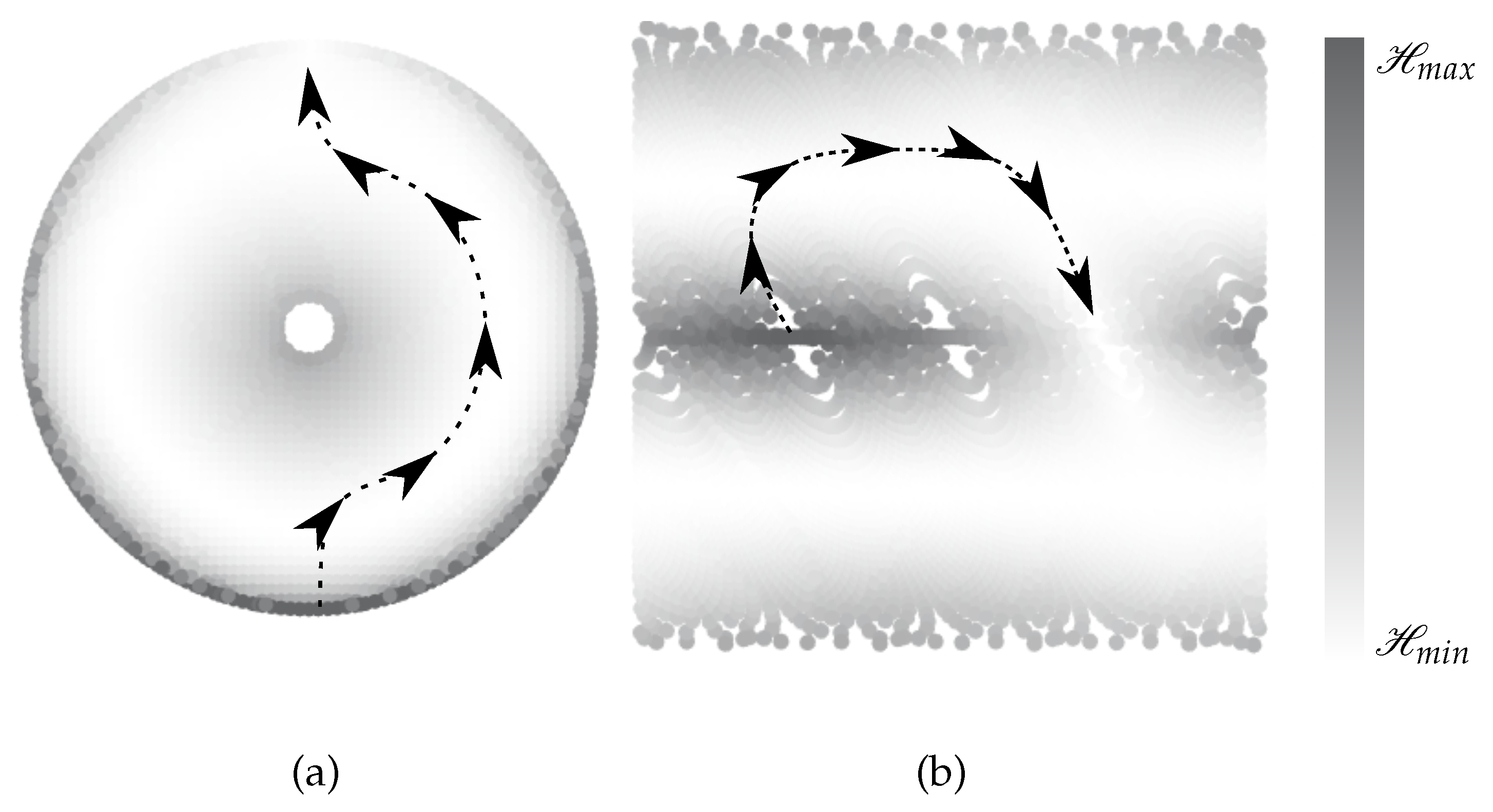
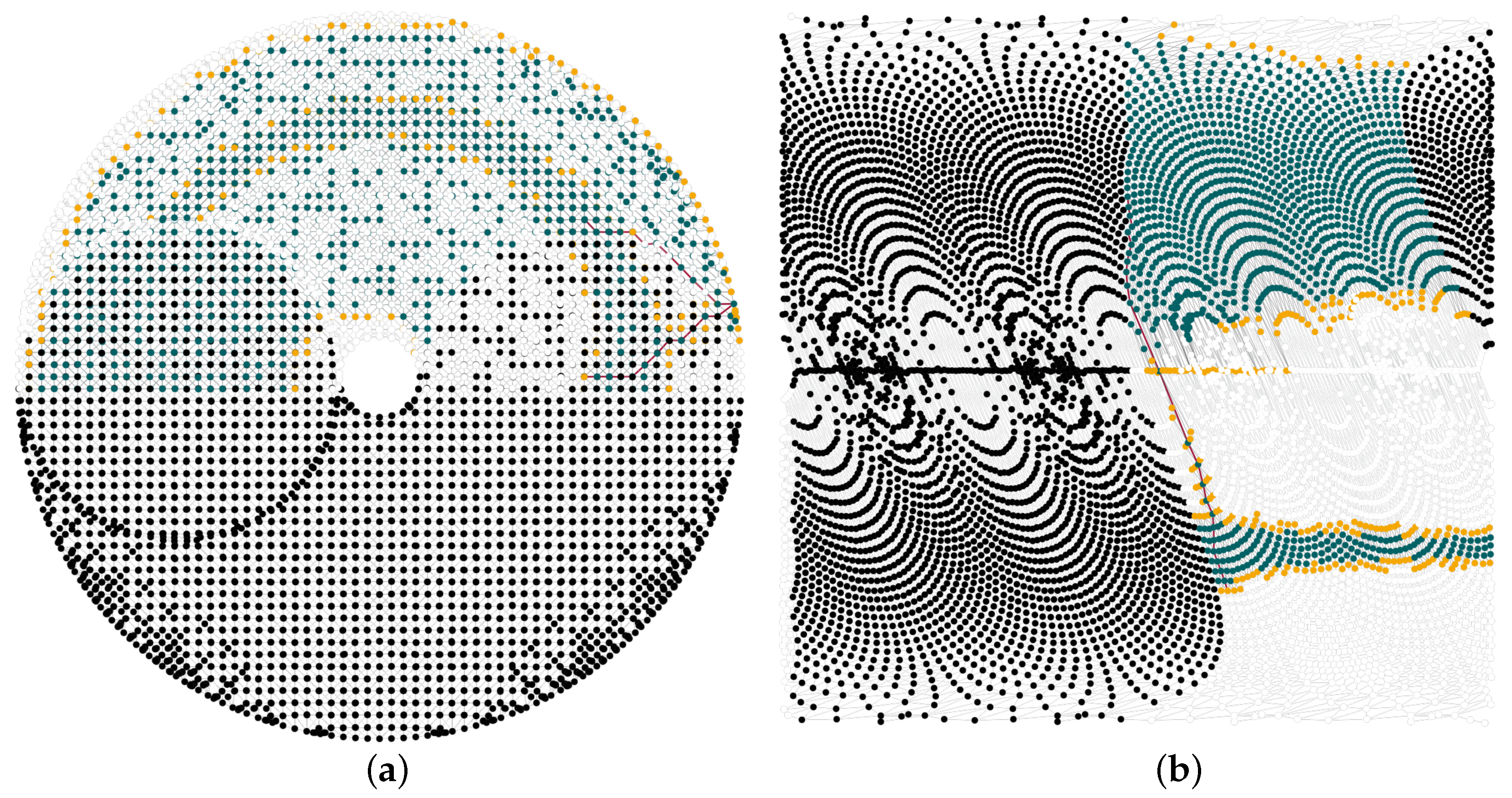
3.1. Shape of the Kinematic Graph

The KG contains the information from both C -space and T -space, and thus can be plotted in both spaces. An exemplarily sketch of the KG is depicted in Figure 5 in Section 3.4. Figure 5a demonstrates the plot of the graph based on the average Cartesian coordinates of the P w in T -space. To make the overlaying vertices V k (clusters) visible, a small offset is imposed. Figure 5b demonstrates the KG in C -space, which can also be interpreted as the “unfolded” version of the KG in T -space. An overview of the colour coding related to the search algorithm is presented in Section 3.4.

3.2. Computational Complexity

Theoretical worst-time computational complexity, with the assumption that the algorithm has to explore the entire graph to find the optimal solution, of the search algorithms is O ( b d ) . In this expression, b is the branching factor and is determined by the average number of neighbours, or successors, of a vertex in the graph in which the search is performed, and d is the solution depth, that is, the shortest path between the start and the goal vertices. This notation may seem to be not of much use though, except that, due to the exponential relation between b and d, it is clear that solving problems with significant b and d values, as in the case of sampling-based planning algorithm for robotic manipulators with articulated arms, becomes computationally intangible. This fact is the most referenced barrier of utilisation of such algorithms for manipulation problems (see Section 1.1). This worst-time computational complexity provides us, however, with some intuition to evaluate the KG.

3.2.1. Branching Factor

Based on the Moore neighbourhood strategy, the number of neighbours of a state in a two-dimensional (2D) problem, e.g., the positioning problem of a planar mechanism or a holonomic mobile robot, is eight. This is implied from the fact that the state of each dimension can remain unchanged or can move in positive and negative directions (restrictions apply at the boundaries). Hence, the simple formula of
b = | s u c c _ s t a t e s | d i m 1 ,
where | s u c c _ s t a t e s | is the number of the successor states of each one-dimensional action that can be derived to evaluate the average number of neighbours of a state (for a 2D problem: b = 3 2 1 = 8 ).
Obviously, the branching factor increases exponentially. For a three-dimensional (3D) problem, the branching factor will be b = 3 3 1 = 26 . In the case of 6D manipulation problems, the branching factor will be b = 3 6 1 = 726 . The essential effect of dividing the problem into positioning and orientation and applying the sampling-based planning algorithm for the positioning problem, can now be inferred.

3.2.2. Solution Depth

The significant reduction in the dimension of the problem based on the clustering can basically be deduced from Algorithm 1. In this Section, we attempt to present a quantification of this result. Let us consider a planar two-DoF mechanism. Although the topology of the C -space of this mechanism is of non-Euclidean shape (it has the shape of a torus), it can be parametrised and represented as a 2D Euclidean space, with axes of θ 1 and θ 2 . The construction of the KG can be regulated based on two parameters: C res and T res . For the sake of simplicity, let us consider the same limits for the joints of the mechanism, θ 1 , θ 2 [ π , π ] T , [ π , π ] T . A specific number of joint values ( | j v | ) will be generated, based on deterministic regular discretisation of the joint range and C res . For instance, for C res = π , | j v | { C res = π } = 3 . Let us consider three different C res = 2.0 , 1 . 0 , and 0.5 . Then, | j v | { C res = 2 . } = 181 , | j v | { C res = 1 . } = 361 , and | j v | { C res = . 5 } = 721 .
The first step of the construction of the KG is generating a C -space graph, G C ( V C , E C ) . Based on the Moore neighbourhood strategy, the number of vertices ( V C ) and edges ( E C ) of this graph can be computed as follows (note that this is physically an undirected graph) [41]:
V C = | j v | 2 ,
and,
E C = 4 | j v | 2 6 | j v | + 2 .
Thus, V C { C res = 2 . } = 32,761, V C { C res = 1 . } = 130,321, and V C { C res = . 5 } = 519,841. Also, E C { C res = 2 . } = 129,960, E C { C res = 1 . } = 519,120, and E C { C res = . 5 } = 20,570,440.
Now we continue to generate the G k V k , E k by regulating the second parameter, T res . We consider four different T res = 0.1 m (coarse) , 0.05 m , 0.03 m , and 0.01 m (fine). The number of the vertices and edges, V k and E k respectively, generated via Algorithm 1 and the relation between the number of the dimensions of G k and the underlying G C are summarised in Table 1. For the examples in the following sections, the applied resolutions for contraction of the KG are C res = 1 . and C res = 0.05 .
For most (almost all well-determined) pairs of C res and T res the values of the third and fifth columns are rather small, suggesting that the KG, G k , is much smaller than its underlying joint space graph, G C . This is, however, not a surprising result, and merely a quantification of the logic of construction of the KG. This also has a tremendous effect on the reduction in the storage size of the KG, enabling us to store more information, such as the ones that are necessary for direct collision checks in T -space and hence preventing overhead computation time for calling K functions in online applications.

3.3. Cost and Heuristic Functions

To calculate the costs of the transitions between different states C and C (where C is a successor of C , i.e., C succ ( C ) ) and the heuristic functions (which estimate the cost of the shortest path from each state to reach the goal), metric functions are to be determined (see Section 1.3.2) that are quantitatively dependent on the states themselves. Logically, the first pair of choices to be stored in each state are the averaged values of the Cartesian coordinates of the P w
C . pos = N C . pos ¯ ,
and joint states
C . q = q N C ¯ .
Moreover, the average Cartesian coordinates of any critical point on the mechanism can also be stored, as an example of such, the Cartesian coordinates of the elbow of the articulated arm. This specific information will help twofold: (i) checking the collision states directly in T -space (see Section 3.4) and (ii) determining the influence of the arm orientation during the planning for the orientation problem of the wrist.
The above local information can be utilised to determine the cost and heuristic functions based on different distance metrics, such as the Euclidean norm in the corresponding spaces. In addition to this local information, any other indicator based on kinetic, kinematic, or kinetostatic performance criteria can be stored in the KG to achieve a desired motion. It is important to note that the heuristic-based search algorithms require admissible and consistent heuristic functions. This is fulfilled when the amount of the heuristic function in each state does not overestimate the cost of the shortest path from each state to reach the goal and consequently amounts to zero at the goal state.
The commonly used evaluation criteria in the literature are predominantly devoted to the kinetostatic performance values, specifically the manipulability of the robotic manipulators (see, e.g., [30], Section 5.8). These criteria are fundamentally functions of the Jacobian matrix of the manipulators, J , and can generally be split into positional and orientational parts. The geometrical shape of these manipulabilities are ellipses (2D) or ellipsoids (3D). The direction and the length of the principal semi-axes of these ellipses/ellipsoids evaluate the quality of velocity transmission in the corresponding directions. Hence, this provides us with a good measurement for evaluate the distance to the singularities (where the area/volume vanishes) and the directions that lead to them. There can be different measures defined for quantifying the manipulability ellipsoids based on the singular values of J , i.e., the eigenvalues of J J T . The computationally favourable index is the area/volume of the ellipses/ellipsoids, which amounts to
μ = J J T ,
where refers to the determinant of the matrix • ([14], Section 5.4). Henceforth, in the balance of this article we refer to this measure when the manipulability of mechanism is mentioned.
Based on different metrics that one may use in the planning process, distinct evolution of configurational motion is expected for the motions with similar start configurations to the goal posture of the end-effector. Furthermore, the computation time, i.e., the amount of the exploration of the search space to find the optimal motion, is primarily dependent on the selected criteria. Figure 2 demonstrate four different motions of a two-DoF planar mechanism with similar start configurations and the goal postures of the end-effector. The trace of the path of the end-effector ( τ : 0 , 1 T ) is demonstrated with solid lines evolving from green to grey. Obviously, these heuristic function fulfil the conditions of the admissibility of the heuristic functions for the heuristic-based search algorithms in the corresponding spaces in which they are defined.
When the costs and heuristic functions are set to be the distances in C -space, merely 8.36 % of the search space is explored. This amount rises to 17.34 % for the case of T -space exploration. It should be noted that, as mentioned in Section 1.1, it is desired not to call on the IK. However, this is necessary to be able to calculate the C -based heuristics in this scenario. Here, in this example and the example shown in Figures 4b and 6b, we use the C -based heuristics just for demonstrative purposes. Nevertheless, it is observable in the literature that these heuristics has been utilised often. This is not of a great importance in practical scenarios, however, because the KG enables us to use powerful heuristics based on T -space and other performance criteria of the mechanisms.
Now, let us consider a combinatorial pair of costs and heuristics: distance travelled in T -space and the manipulability of the mechanism. Here, special attention should be devoted to this combination. The main task of the heuristic function is guiding the search towards the goal posture of the end-effector, where the function’s value is zero. This seems to be trivial in the context of heuristic functions that are a function of the distances travelled in C -space and T -space: the functions sink towards the goals, and the distance yet to be travelled to reach the goal at the goal posture of the end-effector is zero. The distributions of the manipulability in T -space are, however, geometrically in hyperbolic shapes of different dimensions. Hence, a simple distance function leads the search either to the portions of the T -space with higher manipulabilities or even to singularities. Nonetheless, a combination is very beneficial. For instance, we can exploit the distance function in T -space to provide information on the direction of the exploration towards the goal and ensure the admissibility of the heuristic function and a reformed manipulability function to guide the search towards the portions of the T -space with higher manipulabilities. Examples of such are
C C , C = C . pos C . pos 2 2 μ m a x μ C . q ,
and
H C = P w g . pos C . pos 2 2 μ m a x μ C . q ,
with P w g . pos and 2 representing the goal postures of the points P w and l 2 Euclidean norm, respectively. Alternatively, the inverse of the maximum manipulability (of course not at and near the configuration singularities) can be used. The flow of the heuristic for the combinatorial case of Figure 2d is illustrated in Figure 3. The arrows and the dotted line on the diagrams show, qualitatively sketched, the path of the end-effector (in the C -space and the T -space, respectively) that the planner outputs. Note that the amount of heuristic at the goal posture of the end-effector is equal to zero. In this case, 20.91 % of the search space was explored. Qualitatively, however, this motion is the most “natural” motion generated amongst the previous motions.

3.4. Collision Avoidance

In the conventional approaches of sampling-based planning algorithm, explicit transformations of the obstacles from O -space to C -space are not performed. Instead, Boolean checks should be conducted to examine whether a specific configuration causes any collision in O -space. Hence, a call to K is inevitable. Geometrical relations are followed to determine the spatial occupation of the bodies of the mechanism.
When planning using the KG, we are able to store the necessary information of critical points of the mechanism (see Section 3.3). The construction of the KG is conducted a priori, and thus, in online applications the Boolean collision checks reduce to the geometrical calculations to determine the spatial occupation of the mechanism that can be directly performed in O -space. Therefore, planning using KG outperforms conventional planning in C -space in terms of computational efficiency for collision detection in online single-query applications.
Figure 4 demonstrates cases where there is a O -space obstacle in the T -space of the mechanism. For this scenario, it is not possible to plan a feasible motion using purely the T -space information. The meaning of the colours are the same as those in Section 3.3.
To provide the reader with a better intuition on the KG and the result of the search, Figure 5 details the results of the plan of Figure 4d. In this demonstration, the obstacle is mapped entirely into the KG, and the collision check does not follow the instruction described above for online single-query applications. The black vertices are those that cause collision with obstacles, the green vertices are those that are expanded during the search, and the yellow vertices are those that are met (are in priority queue) but not expanded. The paths are shown in red.
Close investigation of these figures reveal the properties of the KG detailed in the balance of this article. As an example, observe the vertices with the same T -space Cartesian coordinate (i.e., the overlay in T -space), of which some may cause collision (with configurational interpretation of “elbow-down” in this case) and some may lie on the path (with configurational interpretation of “elbow-up” in this case).

3.5. Limitation of Kinematic Graph

3.5.1. “Holes” in the Kinematic Graph

The construction of the KG is subject to the regulation of two parameters: C res and T res . Whereas C res determines with which and how many, if any, configurations the structure reaches the spatial regions of the T -space, T res determines the size of the clusters. If there are no configurations that reach a specific segment of the T -space where voxels are generated based on T res , these voxels remain empty, which results in generation of “holes” in the T -space representation of the KG. This phenomenon occurs basically when the C -space is sampled “coarsely” and the T -space is sampled “finely”. This can lead to a problem where no start index can be found in the KG in the case that the point P w lies on a “hole” at the start configuration of the mechanism because this voxel does not belong to the approximated T -space, i.e., no index c idx can be found to start the search.

3.5.2. Sparsity in Configuration Space

A feasible path is the one that can be traced by the mechanism, that is, the one that takes the physical limitation of the actuators of the mechanism into consideration. The path planner, hence, should generate paths that correspond to configurational executable motions of the mechanism from the start configuration to the goal posture of the end-effector. Due to the clustering process, the C -space representation of the KG can be sparse in the vicinity of the configuration singularities of the mechanism. This phenomenon can be comprehended by inspection of Figure 5b. The reason for this phenomenon is the small change in the position of point P w in the C -space in the vicinity of the singularities. As the clustering was performed based on the movements encoded in the T -space, if a path traverses in the vicinity of a configuration singularity, or passes through it, moving from one cluster to the next, it demands large steps in the C -space. This may lead to violation of the physical limitation of the actuators of the mechanism. It is worthwhile to mention that this is an essential limitation due to the configuration singularity of the mechanism and can be mitigated by performing interpolation on the generated path segments in post-processing steps. Besides that, collision avoidance in the path segments should be given due attention (see, e.g., [5], Section 5.3.4).

3.5.3. Completeness

The method developed in this article is primarily suitable for the positioning problem of robotic manipulators. The consideration of the problem as a decentralised problem for positioning and orientation is given, based on the discussions of Section 1.1. As discussed in Section 3.2.1, this has a significant effect on the simplification of the problem. However, when solving the problem for the whole manipulator (regional and local structure), the completeness of the algorithm can be guaranteed merely for the positioning problem. This is, however, a theoretical limitation, and not a practical one [20].

4. Applications

Application of the KG will be extended in this section to the more practical cases of robotic manipulators, specifically the ones introduces in Section 1.3. We mention different practical issues that the reader may face during the implementation of the KG and convey the experienced best practices to facilitate the implementation of KG.

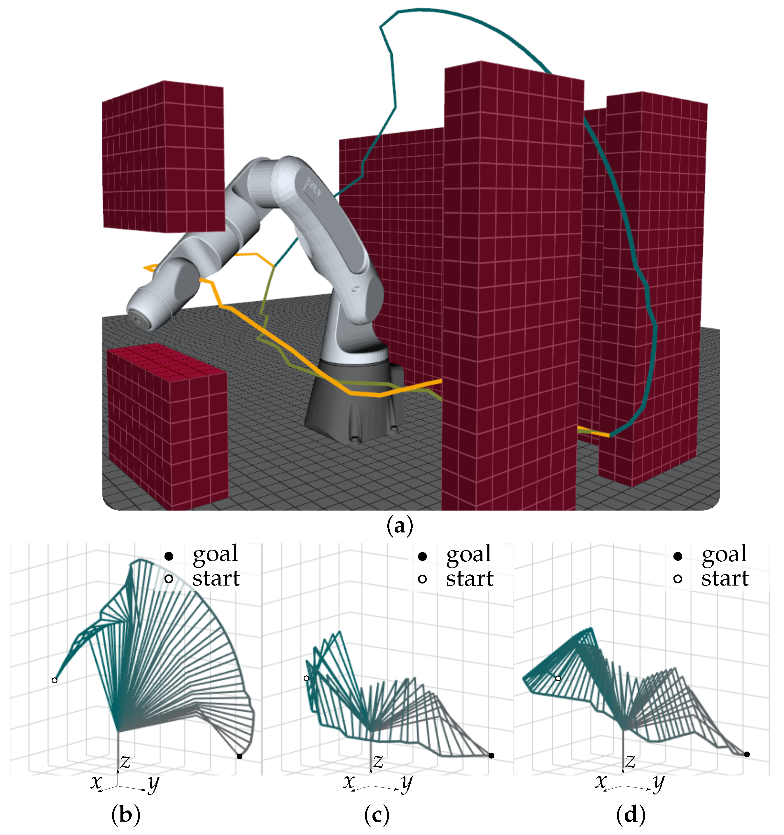
4.1. Implementation for Spatial Robotic Manipulators

Let us start with examples that demonstrate the application of the KG for spatial manipulators. For the examples in this section, we again consider the same cost and heuristic functions introduced in Section 3.3.
In the examples, we simulate a relatively cluttered environment to challenge the search algorithm (see Figure 6a). The meaning of the colours are the same as those in Section 3.3. A quick comparison of the results of these experiments reveal some similarities with those demonstrated in Figure 2. For instance, when the costs and heuristics are set to be the minimum distance travelled in C -space, the manipulator tends to move across the borders of its O -space, minimizing the movements in C -space while sacrificing the manipulability. The behaviour in the case of minimum distance travelled in T -space is also comparable to that of the 2D scenario, moving in the vicinity of the base of the manipulator. Additionally, the combination of cost and heuristic functions based on T -space information and manipulability of the manipulator results in the most “natural” and “predictable” behaviour of the manipulator.

4.2. Best Practices for Implementation of the Kinematic Graph

4.2.1. Finding the Start Index in the Kinematic Graph

In the initial configuration ( q i ), the Cartesian position of point P w may not be of much use to determine the start index in KG, as there may be several vertices (clusters) at the same position (due to reachability of the position with several configurations). In this case, the start index c idx is the answer to the optimisation function
c idx = arg min c idx q i C . q .

4.2.2. Finding the Goal Vertex When Planning in Configuration Space

If the Cartesian posture of the goal ( P w g . pos ) is determined in T -space but the attempt is to plan a path in the C -space, the voxel v in which the goal posture finds itself can be found via
P w g . pos v . cent T res 2 .
The vertices with the same v . cent are the potential goal vertices in the KG, and the one with the least Euclidean norm of the distance from q i to C . q (minimal geodesic on C ) is the actual goal vertex in the C -space, if the minimal geodesic is collision-free. This may be helpful when the calculation of heuristic functions from C -space is desirable.

4.2.3. Defining the Stop Criteria When Planning Explicitly in Task Space

The planning procedure returns a path when some condition at the goal posture of the end-effector is satisfied. If the goal posture is explicitly given as P w g . pos , then the computation of the path is concluded when
C . v . cent P w g . pos 2 2 δ ,
with δ being a small positional tolerance. This is the case for the mechanisms designed for positioning tasks.

4.2.4. Defining the Stop Criteria When Planning Implicitly in Task Space

When the goal posture is not given explicitly but the complete posture of the end-effector is, then two conditions should be satisfied:
  • The position of the end-effector ( e e . pos ) should be reachable from P w g . pos , i.e., e e . pos should be on the surface of the sphere/torus-shaped manifold covering point P w ;
  • The collision of the wrist with the articulated arm should be addressed. This check can be performed using the position of the elbow.

4.2.5. Reaching the Goal

When the goal posture of the manipulator is given explicitly in the T -space, it is not likely that the P w g . pos coincides with a vertex of the KG. Nevertheless, the output can be considered as a “perfect” initial guess for the numerical solution of the goal posture. A better practice is, however, using kinematic control loops (see, e.g., [15]). This is done by feeding the post processed path from the sampling-based planning algorithm with the KG by combining it with the motion plan of the wrist into the kinematic control loop.

5. Conclusions

In this article, we have presented a detailed introduction to the structure of novel graph dubbed Kinematic Graph KG. We have analysed the performance of the KG and have shown that the KG holds the premises arisen from the motivation of developing it, including, but not limited to, the following:
  • Any path that is generated using the KG is guaranteed to correspond to a feasible motion that is kinematically and configurationally feasible for the robotic manipulator to execute (however, the issues of collision avoidance in path segments should be considered). That is, planning using the KG is not affected by the hindrances due to the non-injective surjection of the forward kinematics function for mechanisms with open-chain topology, such as robotic manipulators with articulated arms;
  • Using the KG, it is possible to effectively employ sampling-based planning algorithm for robotic manipulators, i.e., the problem of higher dimensions;
  • Using the KG, it is possible to employ cost and heuristic functions for heuristic search algorithms from the combination of the information from C -space and T -space of the robotic manipulators.
Up to now, we have employed cost and heuristic functions based on the distances in Euclidean spaces of C -space representation and T -space. In our future research, we will attempt to integrate the costs and heuristics based on kinetic and potential energy in sampling-based planning algorithm using KG.

Author Contributions

B.C.: supervision, project administration, and funding acquisition. A.S.: conceptualisation, methodology, investigation, visualisation, validation, and writing—original draft preparation; B.C. and A.S.: writing—review and editing. All authors have read and agreed to the published version of the manuscript.

Funding

Funded by the Deutsche Forschungsgemeinschaft (DFG, German Research Foundation) under Germany’s Excellence Strategy—EXC-2023 Internet of Production—390621612.

Institutional Review Board Statement

Not applicable.

Informed Consent Statement

Not applicable.

Data Availability Statement

Not applicable.

Acknowledgments

The authors would like to thank Vincent Brünjes and Thomas Kinzig for the constructive comments, discussions, and kind support during the software development.

Conflicts of Interest

The authors declare no conflict of interest. The funders had no role in the design of the study; in the collection, analyses, or interpretation of data; in the writing of the manuscript; or in the decision to publish the results.

Nomenclature

The following list of symbols is used in this manuscript:
SymbolDescription
C Configuration space
C free Free C , C free C \ C obs
C res Sampling resolution of C
cent Centroid of the voxel in O
C Cluster of nodes in voxel
c idx Index of a cluster
c A cluster in the set of the cluster objects
C The amount of the cost function
e An edge of a graph
E The edges of a graph
E k The edges of the Kinematic Graph
G A graph
G k The Kinematic Graph
H The amount of the heuristic function
K Forward kinematics ( K : C T )
μ Linear manipulability
N Set of node objects
n A node ∈ N
n idx Index of a node
N C Set of nodes in a cluster C
O Open set of nodes for clustering
P w The centre point of the wrist
pos Cartesian coordinate of the node in O -space
q Generalized coordinates of C
r Reach of the point P w
R Field of real numbers
T Task space
T res Sampling resolution of T
v A vertex of a graph
V The vertices of a graph
V k The vertices of the Kinematic Graph
V Set of voxel objects
v A voxel ∈ V
v . N v Set of nodes in a voxel v
O Environment (World)

References

  1. Biagiotti, L.; Melchiorri, C. Trajectory Planning for Automatic Machines and Robots; Springer: Berlin/Heidelberg, Germany, 2008. [Google Scholar]
  2. Lozano-Pérez, T.; Wesley, M.A. An algorithm for planning collision-free paths among polyhedral obstacles. Commun. ACM 1979, 22, 560–570. [Google Scholar] [CrossRef]
  3. Lozano-Pérez, T. A simple motion-planning algorithm for general robot manipulators. IEEE J. Robot. Autom. 1987, 3, 224–238. [Google Scholar] [CrossRef] [Green Version]
  4. Khatib, O. Real-time obstacle avoidance for manipulators and mobile robots. In Proceedings of the 1985 IEEE International Conference on Robotics and Automation, St. Louis, MO, USA, 25–28 March 1985. [Google Scholar]
  5. LaValle, S.M. Planning Algorithms; Cambridge University Press: Cambridge, UK, 2006. [Google Scholar]
  6. Brooks, R.A.; Lozano-Pérez, T. A subdivision algorithm in configuration space for find path with rotation. IEEE Trans. Syst. Man Cybern. 1985, SMC-15, 224–233. [Google Scholar] [CrossRef] [Green Version]
  7. Siciliano, B.; Khatib, O. (Eds.) Springer Handbook of Robotics; Springer International Publishing: Berlin/Heidelberg, Germany, 2016. [Google Scholar] [CrossRef]
  8. Koren, Y.; Borenstein, J. Potential field methods and their inherent limitations for mobile robot navigation. In Proceedings of the IEEE Conference on Robotics and Automation, Sacramento, CA, USA, 7–12 April 1991; Volume 2, pp. 1398–1404. [Google Scholar]
  9. Lindemann, S.R.; LaValle, S.M. Current issues in sampling-based motion planning. In Robotics Research, Proceedings of the Eleventh International Symposium, Siena, Italy, 19–22 October 2003; Springer: Berlin/Heidelberg, Germany, 2005; pp. 36–54. [Google Scholar]
  10. Koenig, S.; Likhachev, M. Fast replanning for navigation in unknown terrain. IEEE Trans. Robot. 2005, 21, 354–363. [Google Scholar] [CrossRef]
  11. Stentz, A. The focussed D* algorithm for real-time replanning. In Proceedings of the International Joint Conference on Artificial Intelligence, Montreal, QC, Canada 20–25 August 1995; Volume 95, pp. 1652–1659. [Google Scholar]
  12. Holladay, R.; Salzman, O.; Srinivasa, S. Minimizing task-space Frechet error via efficient incremental graph search. IEEE Robot. Autom. Lett. 2019, 4, 1999–2006. [Google Scholar] [CrossRef] [Green Version]
  13. Husty, M.L.; Pfurner, M.; Schröcker, H.P. A new and efficient algorithm for the inverse kinematics of a general serial 6R manipulator. Mech. Mach. Theory 2007, 42, 66–81. [Google Scholar] [CrossRef]
  14. Lynch, K.M.; Park, F.C. Modern Robotics, Mechanics Planning, and Control; Cambridge University Press: Cambridge, UK, 2017. [Google Scholar]
  15. Shahidi, A.; Hüsing, M.; Corves, B. Kinematic Control of Serial Manipulators Using Clifford Algebra. IFAC-PapersOnLine 2020, 53, 9992–9999. [Google Scholar] [CrossRef]
  16. Hauser, K.; Emmons, S. Global redundancy resolution via continuous pseudoinversion of the forward kinematic map. IEEE Trans. Autom. Sci. Eng. 2018, 15, 932–944. [Google Scholar] [CrossRef]
  17. Berenson, D.; Srinivasa, S.S.; Ferguson, D.; Collet, A.; Kuffner, J.J. Manipulation planning with workspace goal regions. In Proceedings of the 2009 IEEE International Conference on Robotics and Automation, Kobe, Japan, 12–17 May 2009; pp. 618–624. [Google Scholar]
  18. LaValle, S.M. Rapidly-Exploring Random Trees: A New Tool for Path Planning. 1998. Available online: http://msl.cs.illinois.edu/~lavalle/papers/Lav98c.pdf (accessed on 27 February 2022).
  19. Cohen, B.; Chitta, S.; Likhachev, M. Single-and dual-arm motion planning with heuristic search. Int. J. Robot. Res. 2014, 33, 305–320. [Google Scholar] [CrossRef]
  20. Rickert, M.; Sieverling, A.; Brock, O. Balancing exploration and exploitation in sampling-based motion planning. IEEE Trans. Robot. 2014, 30, 1305–1317. [Google Scholar] [CrossRef]
  21. Scheurer, C.; Zimmermann, U.E. Path planning method for palletizing tasks using workspace cell decomposition. In Proceedings of the 2011 IEEE International Conference on Robotics and Automation, Shanghai, China, 9–13 May 2011. [Google Scholar] [CrossRef]
  22. Mesesan, G.; Roa, M.A.; Icer, E.; Althoff, M. Hierarchical path planner using workspace decomposition and parallel task-space rrts. In Proceedings of the 2018 IEEE/RSJ International Conference on Intelligent Robots and Systems (IROS), Madrid, Spain, 1–5 October 2018; pp. 1–9. [Google Scholar]
  23. Yang, Y.; Merkt, W.; Ivan, V.; Li, Z.; Vijayakumar, V. HDRM: A Resolution Complete Dynamic Roadmap for Real-Time Motion Planning in Complex Scenes. IEEE Robot. Autom. Lett. 2017, 3, 551–558. [Google Scholar] [CrossRef] [Green Version]
  24. Denavit, J.; Hartenberg, R.S. A kinematic notation for lower-pair mechanisms based on matrices. J. Appl. Mech. 1955, 22, 215–221. [Google Scholar] [CrossRef]
  25. Khalil, W.; Kleinfinger, J. A new geometric notation for open and closed-loop robots. In Proceedings of the 1986 IEEE International Conference on Robotics and Automation, San Francisco, CA, USA, 7–10 April 1986; Volume 3, pp. 1174–1179. [Google Scholar]
  26. Angeles, J. Rational Kinematics; Springer: New York, NY, USA, 2013; Volume 34. [Google Scholar] [CrossRef]
  27. Khalil, W.; Dombre, E. Modeling Identification and Control of Robots; CRC Press: Boca Raton, FL, USA, 2002. [Google Scholar]
  28. Uicker, J.J.; Ravani, B.; Sheth, P.N. Matrix Methods in the Design Analysis of Mechanisms and Multibody Systems; Cambridge University Press: Cambridge, UK, 2013. [Google Scholar]
  29. Müller, A. Screw and Lie group theory in multibody kinematics. Multibody Syst. Dyn. 2018, 43, 37–70. [Google Scholar] [CrossRef] [Green Version]
  30. Angeles, J. Fundamentals of Robotic Mechanical Systems; Springer: Berlin/Heidelberg, Germany, 2007. [Google Scholar]
  31. Elbanhawi, M.; Simic, M. Sampling-based robot motion planning: A review. IEEE Access 2014, 2, 56–77. [Google Scholar] [CrossRef]
  32. Dijkstra, E.W. A note on two problems in connexion with graphs. Numer. Math. 1959, 1, 269–271. [Google Scholar] [CrossRef] [Green Version]
  33. Hart, P.E.; Nilsson, N.J.; Raphael, B. A formal basis for the heuristic determination of minimum cost paths. IEEE Trans. Syst. Sci. Cybern. 1968, 4, 100–107. [Google Scholar] [CrossRef]
  34. Likhachev, M.; Gordon, G.J.; Thrun, S. ARA*: Anytime A* with provable bounds on sub-optimality. In Proceedings of the Advances in Neural Information Processing Systems, Vancouver, BC, Canada, 8–13 December 2003; pp. 767–774. [Google Scholar]
  35. Koenig, S.; Likhachev, M.; Furcy, D. Lifelong Planning A*. Artif. Intell. 2004, 155, 93–146. [Google Scholar] [CrossRef]
  36. Koenig, S.; Likhachev, M. D* Lite. Aaai/iaai 2002, 15, 476–483. [Google Scholar]
  37. Kavraki, L.E.; Svestka, P.; Latombe, J.C.; Overmars, M.H. Probabilistic roadmaps for path planning in high-dimensional configuration spaces. IEEE Trans. Robot. Autom. 1996, 12, 566–580. [Google Scholar] [CrossRef] [Green Version]
  38. Pearl, J. Heuristics: Intelligent Search Strategies for Computer Problem Solving; Addison-Wesley Longman Publishing Co., Inc.: San Francisco, CA, USA, 1984. [Google Scholar]
  39. Shahidi, A.; Kinzig, T.; Hüsing, M.; Corves, B. Kinematically Adapted Sampling-Based Motion Planning Algorithm for Robotic Manipulators. In Advances in Robot Kinematics; Springer International Publishing: Cham, Switzerland, 2022; Volume 24, pp. 453–461. [Google Scholar] [CrossRef]
  40. Peixoto, T.P. The Graph-Tool Python Library. 2017. Available online: https://doi.org/10.6084/M9.FIGSHARE.1164194.V14 (accessed on 27 February 2022).
  41. Kinzig, T. Search-Based Path Planning for Positioning of Robot Manipulators. Master’s Thesis, RWTH Aachen University, Aachen, Germany, 2021. [Google Scholar]
Figure 1. IGOR: the open-chain robotic manipulator designed at IGMR (a) with spherical wrist; (b) with non-spherical wrist.
Robotics 11 00105 g001
Figure 2. The motion of a two-DoF planar mechanism. (a) Cost and heuristic functions: distance in T -space. (b) Cost and heuristic functions: distance in C -space. (c,d) Cost and heuristic functions: combination of the distance in T -space and the linear manipulability of the mechanism.
Robotics 11 00105 g002
Figure 3. The flow of heuristic as combination of distance in T -space and linear manipulability of two-DoF mechanism. (a) T -space representation. (b) C -space representation.
Robotics 11 00105 g003
Figure 4. The motions of two-DoF planar mechanism in presence of a O -space obstacle; (a) Cost and heuristic functions: distance in T -space. (b) Cost and heuristic functions: distance in C -space. (c,d) Cost and heuristic functions: combination of the distance in T -space and the linear manipulability of the mechanism.
Robotics 11 00105 g004
Figure 5. Demonstration of the complete KG G k V k , E k , involving search results for the example of Figure 4d. (a) Demonstration of the KG in T -space (for the vertices with the same Cartesian coordinate a small offset is imposed to avoid complete overlap). (b) Demonstration of the KG in C -space.
Robotics 11 00105 g005
Figure 6. Examples of implementation of the sampling-based planning algorithm for the spatial robotic manipulator IGOR. (a) The oblique view of the experimental set up. (b) Cost and heuristic functions: distance in C -space. Amount of exploration: 22.66 % of the KG (the output path of the P w in the T -space is shown in Figure (a) in dark green). (c) Cost and heuristic functions: distance in T -space. Amount of exploration: 4.69 % of the KG (the output path of the P w in the T -space is shown in Figure (a) in light green); (d) Combination of distance in T -space and linear manipulabilities of the mechanism based on (12). Amount of exploration: 11.3 % of the KG (the output path of the P w in the T -space is shown in Figure (a) in orange).
Robotics 11 00105 g006
Table 1. Quantified evaluation of the size of the KG.
C res | T res V k V k V C E k E k E C
2. | 0.15810.017717450.0134
2. | 0.0524410.074572890.0561
2. | 0.0365790.200823,1530.1782
2. | 0.0130,5610.9328120,3030.9257
1. | 0.16010.004617600.0034
1. | 0.0523890.018371340.0137
1. | 0.0365340.050119,5970.0377
1. | 0.0164,3480.4937237,5160.4575
0.5 | 0.15770.001117048.3e-5
0.5 | 0.0523530.004570310.0003
0.5 | 0.0365100.012519,6350.0009
0.5 | 0.0157,8270.1112183,8430.0089
Publisher’s Note: MDPI stays neutral with regard to jurisdictional claims in published maps and institutional affiliations.

