Article

Optimizing Cycle Time of Industrial Robotic Tasks with Multiple Feasible Configurations at the Working Points

1
Department of Industrial Engineering, University of Padova, 35131 Padova, Italy
2
Department of Management and Engineering, University of Padova, 36100 Vicenza, Italy
*
Author to whom correspondence should be addressed.
Robotics 2022, 11(1), 16; https://doi.org/10.3390/robotics11010016
Submission received: 8 November 2021 / Revised: 24 December 2021 / Accepted: 13 January 2022 / Published: 15 January 2022
(This article belongs to the Topic Industrial Robotics)

Abstract

:
Industrial robot applications should be designed to allow the robot to provide the best performance for increasing throughput. In this regard, both trajectory and task order optimization are crucial, since they can heavily impact cycle time. Moreover, it is very common for a robotic application to be kinematically or functionally redundant so that multiple arm configurations may fulfill the same task at the working points. In this context, even if the working cycle is composed of a small number of points, the number of possible sequences can be very high, so that the robot programmer usually cannot evaluate them all to obtain the shortest possible cycle time. One of the most well-known problems used to define the optimal task order is the Travelling Salesman Problem (TSP), but in its original formulation, it does not allow to consider different robot configurations at the same working point. This paper aims at overcoming TSP limitations by adding some mathematical and conceptual constraints to the problem. With such improvements, TSP can be used successfully to optimize the cycle time of industrial robotic tasks where multiple configurations are allowed at the working points. Simulation and experimental results are presented to assess how cost (cycle time) and computational time are influenced by the proposed implementation.

1. Introduction

The most common industrial robot applications are related to the handling of products, the welding, and the assembly of parts [1]. In such applications, the performance of the robotic workcell is usually limited by the performance of the robot, i.e., the time required by the robot to move between the points. Moreover, usually, these applications are kinematically redundant; in other words, the robot kinematic chain has more degrees of freedom than those required by the task; thus, the robot can perform the same task with several different configurations at one or more working point. The redundancy is mainly due to the symmetry of the task, in which the products can be handled by rotating around the tool axis continuously, (e.g., when vacuum grippers are used), or by discrete angles, (e.g., when standard grippers with two symmetrical fingers are used); thus, it is possible to rotate 180 around the tool axis to pick up an object. In common industrial installations, redundancy is disregarded. In fact, setting up a new workcell is usually a long and tedious process; thus, it is more important to perform a speedy setup instead of optimizing the robot movements. Fortunately, teach-by-demonstration techniques are gaining in popularity [2], thus speeding up the process while, at the same time, including redundancy [3].
As the same task can be performed with different robot configurations, it is possible to choose such configurations so that the movement between points is optimized, i.e., joint displacement is minimized. Redundant robot movement is a well-known topic in literature [4,5] and has been exploited both for the execution of tasks [6], to promote safe human–robot interaction [7] and to implement multiple robot applications [8].
Many of the aforementioned applications are also flexible in terms of task order. In other words, the overall task can be performed independently from the subtask order. For example, if a robot has to fill a grid with products, the order in which the grid is filled is irrelevant to the overall task (i.e., the entire grid completion). As a result, different subtask orders may result in different task times due to the different sequence of movements between the points. To obtain the best order to fulfill the task, solving the Travelling Salesman Problem (TSP) is a valuable option [9]. Such TSP, which aims at finding the shortest path to visit all the “cities” (i.e., the points) once, has been studied extensively over the years thanks to its wide applicability; in fact, researchers are still proposing novel algorithms to solve this problem as efficiently as possible [10,11,12]. TSP has been used in many fields, such as package delivery [13], in which multiple drones were used to deliver packages to customers at the same time, task scheduling for assembly lines [14], medical waste collection during the COVID-19 pandemic [15,16], and rolling scheduling problem in the production of iron and steel [17]. Moreover, the TSP has been jointed with Genetic Algorithms (GA) to divide the tasks between robots [18], although GA are usually stochastic and may provide different solutions based on the simulation.
However, TSP suffers from a primary disadvantage: in its basic formulation, the path must visit all the cities once; thus, it does not allow for leaving a city unvisited. This major limitation has also been studied in the years. Luo et al. [13] use multiple travelers to reach all the cities; in this sense, each traveler has to reach only a subset of cities. Similar problems have been faced in [19], where multiple layers are considered, and in [20], where each traveler is capable of reaching their own cluster of cities and can also move in a cluster of shared locations available to all the travelers. Li et al. [21] introduced virtual tasks to associate tasks of different orders; these are also grouped into clusters. The proposed methods focus on putting forward a solution that allows for visiting all the cities with multiple travelers. However, in other applications, a designer can be interested in the opposite scenario: visiting only a subset of cities with a single traveler (e.g., to check only a small part of a component for anomalies [22]).
In this paper, we aim to solve this issue, by focusing on a robotic application. In fact, if a redundant application is considered, the robot can reach a point (i.e., a city) with multiple configurations, thus requiring different movement times. As a result, each configuration can be considered a separate city, but the different configurations in the same points are mutual, so the robot must visit one of the possible configurations and not the others. In particular, this paper aims at adapting the TSP to the following scenarios:
  • to find the optimal task order in the case of multiple working points with multiple configurations and no fixed sequence;
  • to find the optimal configurations in the working points with multiple configurations and a fixed sequence.
The paper is structured as follows: Section 2 introduces the complexity of the problem of the multiple-configurations; Section 3 describes the analytical model required to implement the multi-configuration within the TSP; Section 4 shows simulation and experimental results to analyze how both the cost and computational time of the TSP solution are affected by the model parameters. Finally, conclusions are drawn in Section 5.

2. Industrial Robotic Tasks with Multiple Feasible Configurations at the Working Points

Let us consider the problem in which the robot should perform a task composed of N points, where the sequence is not imposed by the task. For example, let us consider a quality inspection where a robot must move a camera around an object from a starting (home) position, taking N 1 shots of the object. In this context, the number of possible paths n N , i.e., the number of possible sequences of points, is as follows [23]:
n N = ( N 1 ) ! 2
as a path is made up of N 1 connections and the direction of the path is not relevant. In fact, Equation (1) holds for an industrial robot, since the joints are actuated by means of electric motors, thus moving from point i to point j has the same cost of the inverse motion. Conservative forces (e.g., gravity) are not relevant, since the TSP provides a closed path. The complexity of the problem (i.e., n N ) greatly increases by increasing the number of points N: for example, 5 points led to n N = 12 , while 10 points led to n N = 181,440 . Hence, it is crucial to find a way of narrowing down the number of possible paths to ensure low computational times.
If a point can be reached with multiple configurations, the number of paths increases. For example, if a single point can be reached with k configurations, each of the paths yielded by Equation (1) must be considered k times; thus, the total number of paths becomes k ( N 1 ) ! / 2 . In fact, in the aforementioned case of the quality inspection, a camera with a rectangular sensor can fulfill the task by taking a photo by rotating 180 about its optical axis (Figure 1). The path must now choose between two configurations ( k = 2 ) for a single point, doubling the number of possible paths.
This situation occurs when either the tool can be placed in different ways or the robotic arm can be posed in different configurations, or both. Indeed, an industrial 6-axis robot is kinematically redundant, as its inverse kinematic problem provides multiple solutions based on the structurally available configurations. For a standard robot, such configurations are commonly related to the shoulder (lefty/righty), elbow (above/below), and wrist (flip/no flip), with a total of eight (8) possible combinations of configurations. In practice, it is often impossible that all the configurations are feasible (due to possible collisions or joint mechanical limits), but among the possible configurations, it is important to choose the one that optimizes robot performance. Particularly, flip/no-flip configurations are usually feasible, as they rarely result in collisions with the environment.
In general, let m i be the number of points with k i multiple configurations and N g 
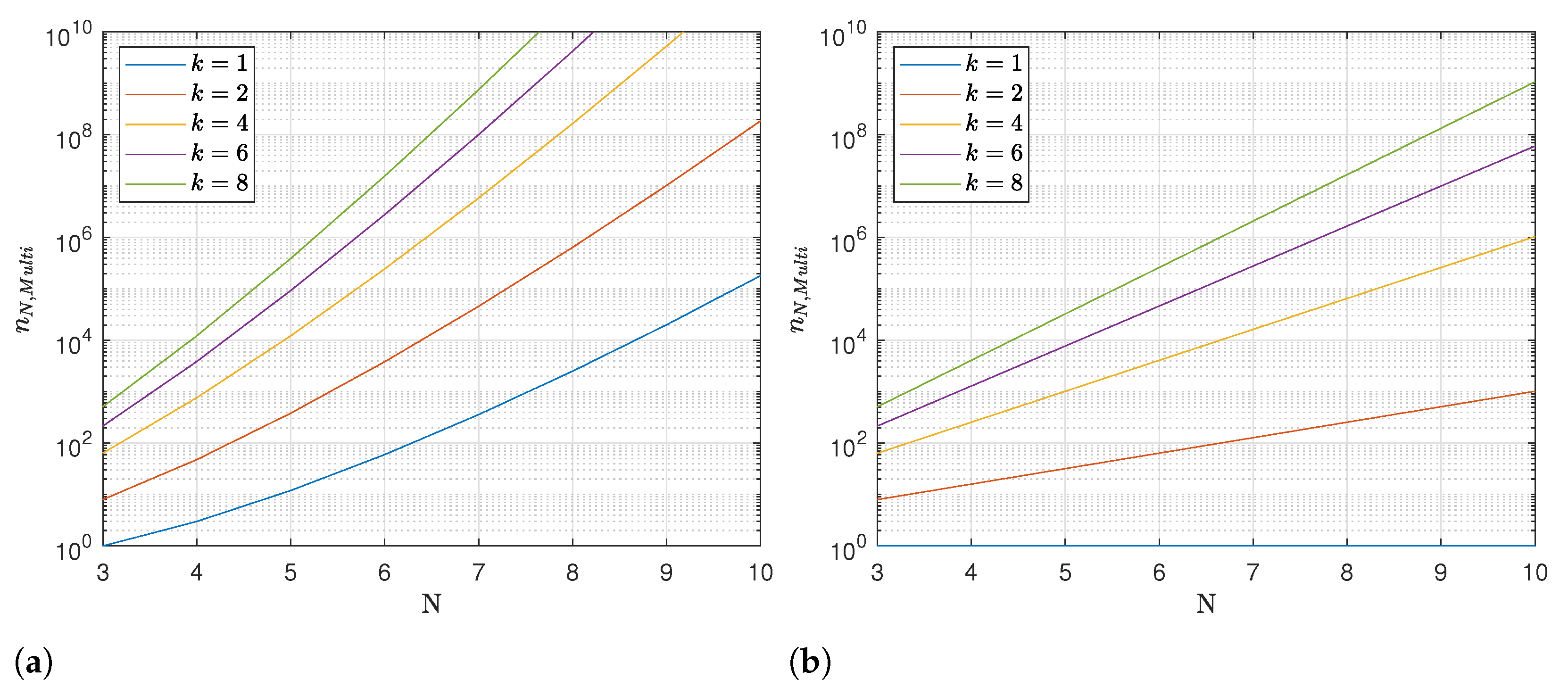
be the number of groups of points holding the same number of configurations. The number of possible paths is as follows:
n N , m u l t i = i = 1 N g k i m i ( N 1 ) ! 2
where i = 1 N g m i = N . Please note that, when all the points allow only one configuration (i.e., N g = 1 , k 1 = 1 , m 1 = N ), Equation (2) yields Equation (1).
The higher the number of configurations for each point, the higher the number of combinations. For example, in Figure 2a, the number of combinations is shown for different k values under the hypothesis that all the points have the same number of configurations (i.e., N g = 1 , k 1 1 , m 1 = N ).
Moreover, even in the case of a fixed point sequence, the number of combinations, in the case of k i > 1 , is not equal to 1. Indeed, a designer could be interested in optimizing the performance of the robot by choosing the appropriate configurations in the case of a fixed robot task order, i.e., when the industrial process is composed of a fixed sequence of subtasks. In this case, Equation (2) can be simplified as follows:
n N , m u l t i = i = 1 N g k i m i
As there is only one fixed point sequence, so the term ( N 1 ) ! / 2 is neglected. Even without the factorial factor of Equation (2), the number of combinations greatly increases with k i (Figure 2b).
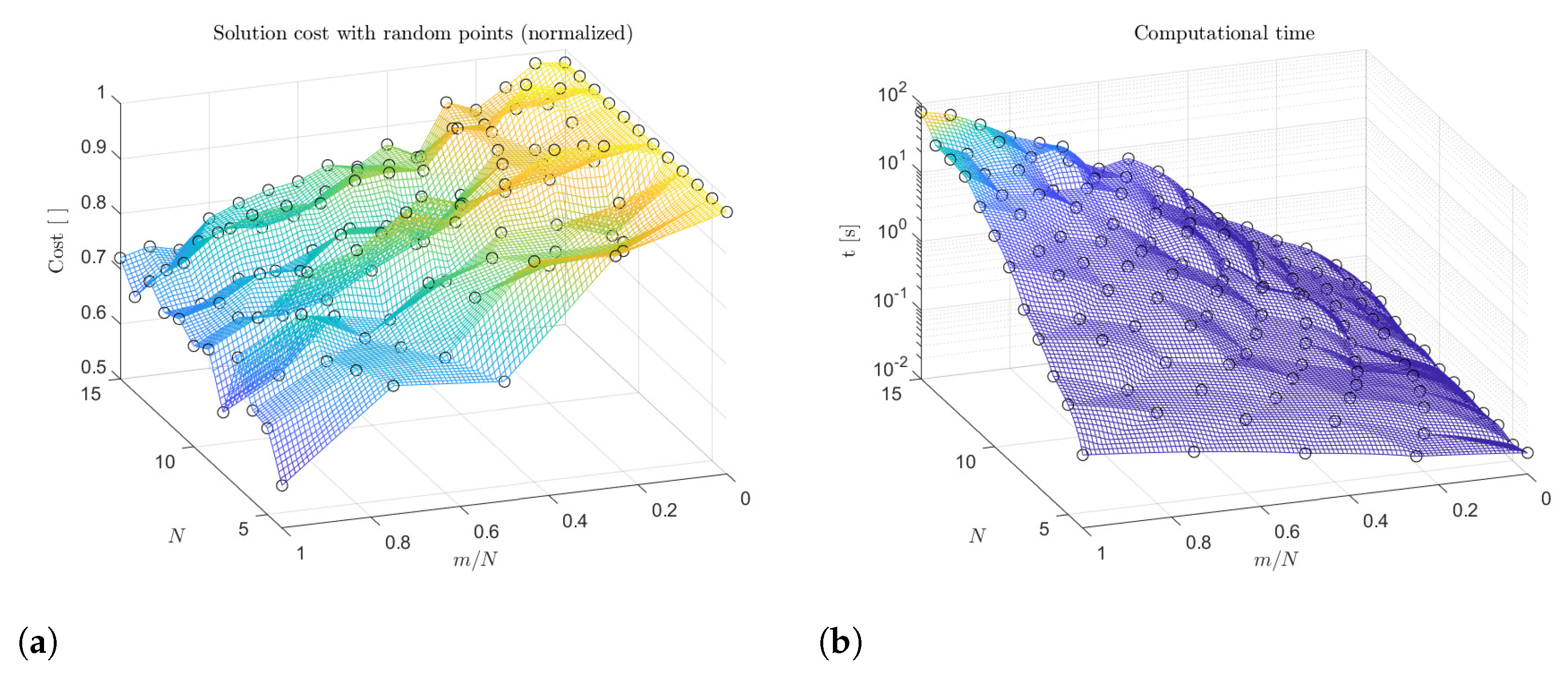
It is worth noticing that an increase in the total number of possible paths is generally followed by an increase in the computational effort required for finding the best solution. However, the increase in computational effort is generally followed by a reduction in the overall solution cost (i.e., a reduction in the robot cycle time). In fact, increasing the number of possible configurations with the same number of points increases the number of combinations and, thus, is likely to find a path that requires a lower cost to be followed.
To verify this reasoning, an industrial 6-axis robot (Adept Viper s650) has been exploited, and 20 simulations have been performed. During each test, N random configurations are chosen in the robot joint space ( k = 1 ); then, the corresponding inverse flip/no-flip robot configurations are calculated ( k = 2 ). Finally, the configurations with ± 180 on the last joint are calculated for both the flip/no-flip configurations ( k = 4 ).
For each value of k, all of the possible path movement times are calculated. Figure 3a shows the ratio between the minimum time of the solution with k > 1 ( t k ) and the minimum time with no multiple configurations ( t 1 , k = 1 ). It is clear how increasing the number of possible configurations changes the minimum possible time; thus, simply by considering different robot configurations, it is possible to reduce the cycle time.
The same trend can be noted if the point sequence is fixed and only the configurations are to be chosen (Figure 3b). It is worth noticing how, in Figure 3a, the ratio t k / t 1 is calculated by taking, for each N, the best solutions with k = 1 and with k 1 , which means that those solutions may be found with different point sequences. In the case of Figure 3b, however, the solutions with k = 1 and with k 1 have the same point sequence; thus, t k / t 1 may reach even lower values. Indeed, it could be possible that the solution with k = 1 is way worse than the one with no fixed point sequence so that t k / t 1 may decrease.

3. Optimizing Cycle Time through the Travelling Salesman Problem

Provided that the task can be fulfilled in n N , M u l t i different ways, optimization techniques such as the TSP can be used to obtain the optimal solution according to a target cost function. The TSP provides the path that connects all the points reducing the cost index. Such a path must visit the points once, and the cost index can be any design target, such as traveling distance, traveling time, and energy consumption. The cost index is usually stored within a square matrix C, in which an element c h k describes the cost in moving from point h to point k. Such cost can be any performance index based on the specific application (e.g., movement time, energy consumption, maximum acceleration, safety index).
The TSP is particularly interesting because it aims at finding the best path among all the possible combinations. Other optimization techniques, such as genetic algorithms, are generally stochastic; thus, it is possible that the calculated solution is not the global optimum. Moreover, increasing the number of configurations has a major drawback: its maximum possible cost increases with k; thus, choosing the wrong path (with a stochastic approach) could not benefit from the increase of k and, conversely, could provide an even more expensive solution (if compared to the case with k = 1 ).
The TSP can be easily applied in the case of Equation (1), as the solution provided passes through all the N points. On the contrary, the application of the TSP in the case of multiple configurations is not straightforward. In fact, the points to be considered are more than N, as multiple configurations must be considered:
N * = i = 1 N g k i m i
However, the solution must encompass only N points. In other words, the solution must not provide a path that passes through the same point with different configurations.
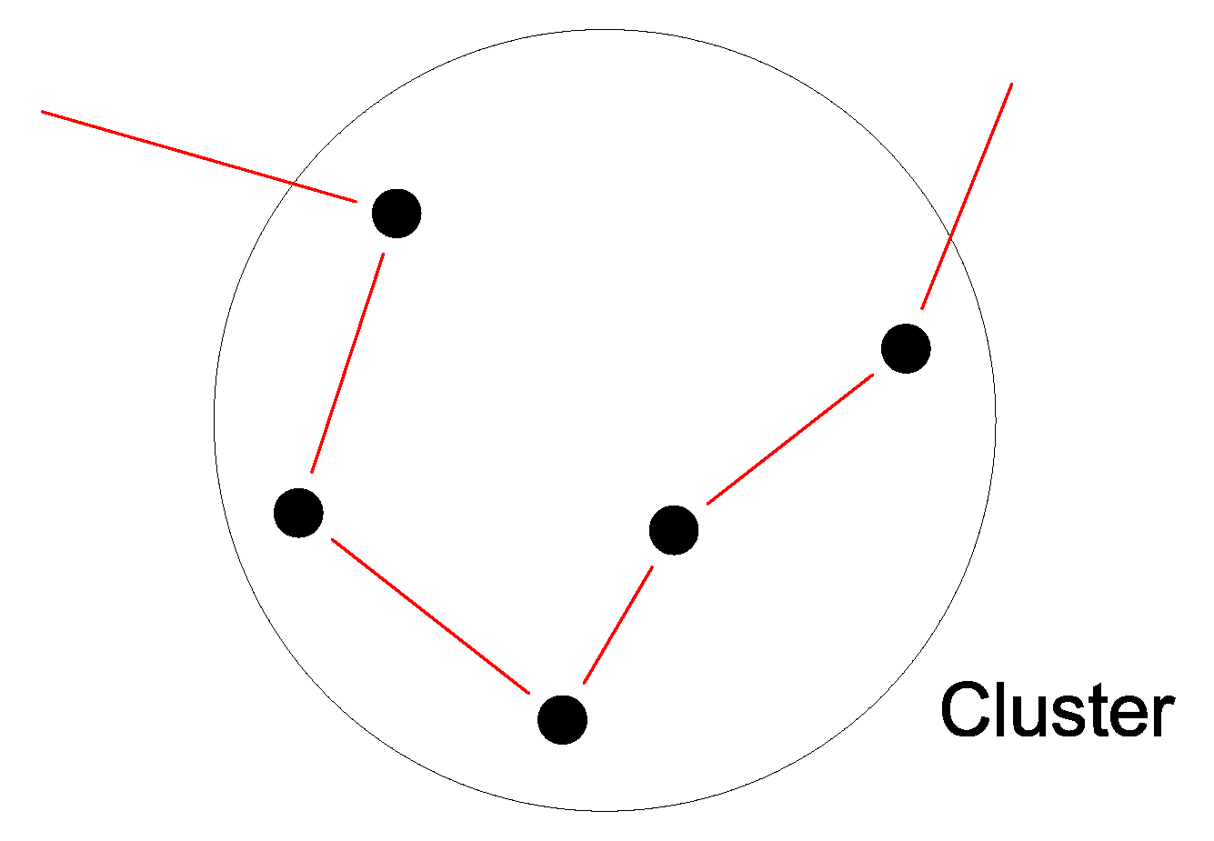
The TSP does not allow for ignoring some points. It is then necessary to improve the algorithm to provide a feasible solution. As shown in a previous work [24], it is possible to divide the positions into clusters. By applying the cluster constraints, the TSP is forced to choose a path that enters a cluster via one point, visits all the other points of the cluster, and exits towards other points (Figure 4).
In this sense, if, for a single point, all the configurations are clustered, the TSP is forced to move to a point, pass through all the configurations, and move to another point. However, it is not possible to simply cluster all the configurations together, as the last configuration of the cluster is different from the first. In fact, it is necessary that the TSP solution enters and exits from the same configuration; otherwise, the final cost would be affected. For example, let us consider the quality inspection case (Figure 1). In taking the photo, the TSP solution must move to the point with a chosen configuration and then move to the next, ignoring the other configurations.
To overcome this issue, mirror copies are introduced. Mirror copies are copies of the existing configurations and are used to avoid discrepancies in the final cost of the TSP solution. As the mirror copies are equal to the configurations, the costs of moving toward the other points are the same. Configurations and mirror copies of the same point are grouped into a cluster. To avoid confusion, the points are named via one single subscript (e.g., P i ); the configurations, with a double subscript ( P i , j ); and the mirror copies, with an asterisk ( P i , j * ).
To obtain a reasonable solution, the TSP must obey to the following constraints in moving to a point with multiple configurations:
  • The path must enter a cluster through one configuration and exit through its mirror copy.
  • To avoid discrepancies in the final cost, the connections within a cluster must have null cost.
To do so, we propose to connect the configurations and the mirror copies in the following way: considering point P i , the j-th configuration ( P i , j ) is connected within the cluster only to its mirror copy ( P i , j * ) and to the mirror copy of the following configuration ( P i , j + 1 * ). The last configuration P i , k is connected to the mirror copy of the first configuration P i , 1 * .
Moreover, we apply some constraints: with reference to Figure 5, the number of blue connections must equal the number of configurations k, while the number of yellow connections must equal k 1 . In total, each cluster contains 2 k 1 connections.
As an example, let us consider Cluster P1 in Figure 5. If the path moves to point P 1 via configuration P 1,1 , it is then forced to move to P 1,2 * , P 1,2 and so on, exiting the cluster from P 1,1 * . As a result, k blue connections and k 1 yellow connections are used. Please notice that it is not possible for the path to move from P 1,1 to P 1,1 * and exit from P 1,2 * , as, in this case, the path would pass through k 1 blue connections and k yellow connections, not obeying the aforementioned constraint.
The introduction of the mirror constraint increases the complexity of the TSP, as the number of cities increases. In fact, it is possible to rewrite Equations (1) and (2) as follows:
n N = [ i = 1 N g ( a i k i · m i ) 1 ] ! 2
n N , m u l t i = i = 1 N g ( a i k i ) m i ( N 1 ) ! 2
where
a i = 2 if the point has more than one configuration 1 otherwise
It is worth noticing that k i must be doubled only when the mirror configurations are needed. Equation (5) is valid with the standard TSP, when no constraints are applied. Otherwise, Equation (6) holds.
Equations (5) and (6) do not provide the same number of possible paths. It is clear how the number of possible paths is greatly reduced by applying the constraints, thus reducing the overall complexity.
The proposed method can be applied also in the case of a working cycle made of a set of Cartesian paths that must be executed in sequence. Let us consider, as an example, a painting task where the painting tool must be moved along certain paths; in such an application, the robot configuration must be kept all along each path, but may change between the exit point of a path and the starting point of the subsequent path. The cycle time can be optimized using the proposed method, by assigning a cluster to each path (Figure 6). The cluster must comprise all the possible configurations of the starting point of the path (instead of the working point), whereas the mirror copies are substituted by the corresponding configurations of the exit point of the path. In this way, the TSP will optimize both the sequence of the paths (clusters) and the robot configuration assigned to each path, while forcing the robot to keep such configuration all along the path at the same time.
Overall, the optimization procedure by means of the modified TSP can be summarized as follows (Figure 7):
  • Define the working positions as Cartesian points ( P i ).
  • Identify the feasible redundant configurations for each point ( P i , 1 m ), excluding the configurations that are outside of robot mechanical limits or that result in collisions with the workcell equipment.
  • Calculate the elements of the cost matrix C. This part can be performed by means of common trajectory optimization algorithms, such as RRT-connect algorithms [25,26].
  • Solve the modified TSP using the feasible configurations and the cost matrix as inputs.
  • Finally, the optimal task sequence is provided.
Please note that the TSP outputs a list of the sequence of configurations P i , j that minimizes the overall cost. Since the TSP requires the path to pass through all the configurations, the output list must be filtered to remove all the unused configurations (including the mirror copies), so that the final list is made of a single configuration per point (i.e., the configurations circled in green in Figure 5).

Optimizing Cycle Time in the Case of a Fixed Point Sequence

Although the TSP is generally used to choose the optimal path, it is possible to use it to choose the configurations used with a fixed point sequence (i.e., with a fixed path). In this case, the number of possible combinations decreases. In fact, as shown in Equation (3), the term ( N 1 ) ! / 2 is related to the number of sequences, which can be neglected in the case of a fixed sequence. As a result, n N = 1 , while Equation (6) can be rewritten as follows:
n N , m u l t i = i = 1 N g ( a i k i ) m i
As shown in [24], it is possible to force the TSP solution to follow a certain path by making it choose a connection between two points, namely P i and P r . To do so, the number of chosen connections between P i mirror copies and P r configurations must be equal to one: consequently, the TSP solution is forced to move from a mirror copy of P i toward a configuration of P r ; then, the solution is forced to exit P r via a mirror copy and move toward the next point. This process can be iterated until the entire sequence is fulfilled.

4. Validation

4.1. Simulation Results

To simulate the modified TSP capabilities, a test has been carried out in a Matlab environment. As the TSP is a general problem and is disjointed from the robot movement, to simplify the test, a random set of Cartesian points has been chosen. The simulations have been carried out on a Windows 10 laptop equipped with an i7-8750H and 16 GB of DDR4 RAM, and for each set of parameters, the simulation has been computed 10 times.
Figure 8 shows the results of the simulations. In particular, Figure 8a shows the cost of the solution provided by the TSP, normalized by the corresponding cost that could be provided by the standard TSP ( m / N = 0 ). By looking at the overall cost (Figure 8a), it is clear how the introduction of multiple configurations greatly reduces the final solution cost. This result was expected, as by introducing new configurations for the same point, the final path can follow new routes, thus reducing the final cost. It is worth noticing that the irregular shape of Figure 8a is due to the randomness of the problem: as stated before, the points for each simulation are chosen randomly in the Cartesian space.
The increase in complexity is followed by an increase in the computational time required to obtain a solution (Figure 8b). The computational time increases greatly when the number of points increases, but even for a mid-range laptop, the time needed to obtain a solution is reasonable even with a high number of points (less than 80 s for the worst-case scenario). Indeed, for most of the combinations of Figure 8b, the computational time is way less than a second.

4.2. Experimental Testing

To test the effectiveness of the proposed method, it has been used in an example of a real case application, in which a robot is used to capture some photos on the sides of a pyramid trunk, where some symbols are placed (Figure 9). The camera is placed perpendicular to the 6-joint axis to improve reachability. The robot is an Omron Adept Viper s650, and the camera used is a monochromatic Allied Vision Pike F-505. The camera sensor is rectangular; thus, the photo can be taken by rotating the camera axis by about 180 . To increase the complexity of the problem, both flip/no-flip configurations are considered. The final objective is to decrease the overall robot movement time.
Overall, the parameters of the problem are shown in Table 1, where the photos are taken atop the pyramid trunk and on three out of four inclined sides. The points are where the photos are taken and are placed at a distance of 100 mm from the pyramid sides (Figure 10). One home position is included in the problem. As a result, n N = 1.3 × 10 35 for the standard TSP (Equation (5)), and n N , m u l t i = 49,152 for the TSP with constraints (Equation (6)).
The experimental test has been carried out as follows: first, the position of the pyramid is measured with respect to the robot base, and the points are consequently defined; then, the simulator (developed in Matlab) calculates all the possible movement costs and the TSP is solved; finally, the optimal list of movements is sent to the robot to check the validity of the solution.
To address the validity of the method, the order provided by the TSP is compared to the order chosen by a human operator. The final movements are very similar (Figure 11); however, their overall costs (i.e., the overall movement time) are fairly different. This is due to the large displacements that the robot joints must traverse between the locations (Figure 12a), which result in wider speed bottlenecks (Figure 12b). As a result, while the optimal movement (Figure 11a) takes 2.92 s, the movement of the operator (Figure 11b) takes 3.18 s, with a reduction of nearly 9%. It is to be categorically noted that this reduction is linked solely to this example: it may vary based on the application. The TSP solution is obtained with a computational time of 1.08 s on a mid-range Windows 10 laptop. The swift calculation makes it possible to use the TSP with the simulator to test different positions of the workpiece in the robot workspace to obtain even better results (as in [27]).
Then, all the feasible paths have been considered to check how the movement time varies by changing the order of the points and by changing the chosen configurations. To do so, three different scenarios have been considered:
  • Each point has a single robot configuration;
  • Each point has two robot configurations (flip/no flip);
  • Each point has two robot configurations (flip/no flip) and the rotation takes place around the camera axis (considered case study).
Such scenarios have been implemented for five tests, each of which has a different pyramid position and rotation.
The results are shown in Table 2 and Table 3. The former table shows how increasing the complexity of the problem (i.e., introducing new configurations for each position) makes it possible to improve the solution provided via the TSP. Indeed, by considering two robot configurations only, the average final solution cost decreases by more than 6%. This result is further improved if the rotation around the camera axis is also considered: the average solution cost is reduced by 7.38%. The latter table (Table 3) highlights the importance of the optimization provided by the TSP. In fact, the TSP solution is generally lower than half of the time required for an average task order for the described case study. This average value has been calculated by considering all the possible task orders, with two robot configurations and two camera rotations.
Finally, the case study has been used to test how the TSP handles the choice of the best configurations in the case of a fixed task sequence. Let us consider the sequence of points 1-2-3-4-5 (Figure 11a). The three aforementioned scenarios have been used in the case of Test 1 of Table 2.
The results (Table 4) show how TSP reduces the overall movement time even in the case of a fixed sequence. This result is very promising, as it can greatly improve the cycle time of an industrial robot without any need for changing the production process. This is because the only change relies on the movement of the robot itself.
The results of the optimization, of course, may be influenced by the environment surrounding the robot: changing the initial and final configurations of a movement results in different trajectories, which may result in collisions between the robot and the environment. A collision check must be performed (like in [28]) before solving the TSP, to validate the connections between the feasible configurations of different working points.

4.3. Applicability of the Modified TSP

The modified TSP becomes more flexible and can be applied to different use case scenarios, in which the optimization of the task cannot be retrieved at a glance by a robot programmer.
For example, in the assembly tasks with multiple feeders and several working positions with multiple configurations, the modified TSP can calculate the optimal task order to improve productivity. In [29], a heat exchanger coil has to be assembled by means of a SCARA robot and a symmetric end-effector. Each heat exchanger coil is made of 40 parts to be inserted (20 of first type, 16 of second type, 4 of third type) and 3 bowl feeders that provide the parts. Moreover, the structure of the SCARA and the symmetry of the end effector provide 4 configurations per position.
In robotic spot welding, the robot may rotate by some degrees around the normal to the welding spot surface. This range of rotation may be discretized, and the TSP can calculate the best configuration at working points to optimize the task. In [30], a welding task is made up of 10 welding spots. Let us assume that each welding spot can be reached with at least 3 configurations. The total number of possible combinations, as of Equation (2) is very high.
Finally, in collaborative applications, redundant robots can be deployed to improve flexibility and safety, since ideally the robot can reach working positions with infinite configurations. Such configurations can be chosen with the aim of improving productivity (reducing movement time between positions) or with the aim of improving safety, to prevent the robot from exerting exceeding forces in specific directions (e.g., directed to the operator). In [31], a collaborative assembly task of 10 positions is simulated. In such an application, the proposed TSP approach can be applied by setting the cost c i j between positions as defined by safety indexes.
All aforementioned examples are summarized in Table 5. It is clear that the implementation of an automatic procedure that considers redundant configurations may be of great importance in several industrial applications. Moreover, the modified TSP can be implemented in pair with well-known optimization algorithms (such as RRT-connect), that can be used for the optimization of a single movement and for the population of the cost matrix C.

5. Conclusions

This paper proposed an improvement to the Traveling Salesman Problem that allows to optimize throughput of a robotic workcell in multi-configuration scenarios, widespread in common industrial robot applications. Such method can be used both in the case of point-to point motions (e.g., quality inspection) and in the case of working cycles made of a set of Cartesian paths (e.g., painting). The mathematical additions to the TSP are fairly simple and are very easy to implement.
The results show how the computational time, which increases with the complexity of the problem, remains reasonable in most cases. Simulation and experimental results show the effectiveness of the method by comparing the cycle time provided by the modified TSP and the one obtained by a task sequence intuitively chosen by a human operator. Moreover, it is shown that even a fixed task sequence (e.g., an assembly sequence) can be improved by means of the modified TSP. Future work will aim to reduce the computational effort required by the algorithm.

Author Contributions

Conceptualization, M.B. and G.B.; methodology, M.B. and G.R.; software, M.B.; validation, M.B., G.B. and G.R.; formal analysis, G.B. and G.R.; investigation, G.B. and G.R.; data curation, M.B.; writing—original draft preparation, M.B., G.B. and G.R.; writing—review and editing, M.B., G.B. and G.R.; visualization, M.B., G.B. and G.R.; supervision, G.B.; project administration, G.R. All authors have read and agreed to the published version of the manuscript.

Funding

This research received no external funding.

Institutional Review Board Statement

Not applicable.

Informed Consent Statement

Not applicable.

Data Availability Statement

Not applicable.

Conflicts of Interest

The authors declare no conflict of interest.

References

  1. International Federation of Robotics. IFR Press Conference. 2020. Available online: https://ifr.org/downloads/press2018/Presentation_WR_2020.pdf (accessed on 7 November 2021).
  2. Billard, A.; Calinon, S.; Dillmann, R.; Schaal, S. Survey: Robot Programming by Demonstration; Technical Report; Springrer: Berlin/Heidelberg, Germany, 2008. [Google Scholar]
  3. Alizadeh, T.; Karimi, N. Exploiting the task space redundancy in robot programming by demonstration. In Proceedings of the 2018 IEEE International Conference on Mechatronics and Automation (ICMA), Changchun, China, 5–8 August 2018; pp. 2394–2399. [Google Scholar] [CrossRef]
  4. Bottin, M.; Rosati, G. Trajectory optimization of a redundant serial robot using cartesian via points and kinematic decoupling. Robotics 2019, 8, 101. [Google Scholar] [CrossRef] [Green Version]
  5. Bottin, M.; Rosati, G.; Cipriani, G. Iterative Path Planning of a Serial Manipulator in a Cluttered Known Environment. Mech. Mach. Sci. 2021, 91, 237–244. [Google Scholar] [CrossRef]
  6. Lu, Y.A.; Tang, K.; Wang, C.Y. Collision-free and smooth joint motion planning for six-axis industrial robots by redundancy optimization. Robot. Comput.-Integr. Manuf. 2021, 68, 102091. [Google Scholar] [CrossRef]
  7. Calinon, S.; Sardellitti, I.; Caldwell, D. Learning-based control strategy for safe human-robot interaction exploiting task and robot redundancies. In Proceedings of the 2010 IEEE/RSJ International Conference on Intelligent Robots and Systems (IROS), Taipei, Taiwan, 18–22 October 2010; pp. 249–254. [Google Scholar] [CrossRef]
  8. Touzani, H.; Hadj-Abdelkader, H.; Seguy, N.; Bouchafa, S. Multi-Robot Task Sequencing & Automatic Path Planning for Cycle Time Optimization: Application for Car Production Line. IEEE Robot. Autom. Lett. 2021, 6, 1335–1342. [Google Scholar] [CrossRef]
  9. Bellmore, M.; Nemhauser, G.L. The traveling salesman problem: A survey. Oper. Res. 1968, 16, 538–558. [Google Scholar] [CrossRef]
  10. Zhang, J.; Hong, L.; Liu, Q. An improved whale optimization algorithm for the traveling salesman problem. Symmetry 2021, 13, 48. [Google Scholar] [CrossRef]
  11. Krishna, M.; Panda, N.; Majhi, S. Solving traveling salesman problem using hybridization of rider optimization and spotted hyena optimization algorithm. Expert Syst. Appl. 2021, 183, 115353. [Google Scholar] [CrossRef]
  12. Agrawal, A.; Ghune, N.; Prakash, S.; Ramteke, M. Evolutionary algorithm hybridized with local search and intelligent seeding for solving multi-objective Euclidian TSP. Expert Syst. Appl. 2021, 181, 115192. [Google Scholar] [CrossRef]
  13. Luo, Z.; Poon, M.; Zhang, Z.; Liu, Z.; Lim, A. The Multi-visit Traveling Salesman Problem with Multi-Drones. Transp. Res. Part C: Emerg. Technol. 2021, 128, 103172. [Google Scholar] [CrossRef]
  14. Bottin, M.; Faccio, M.; Minto, R.; Rosati, G. Sales kit automated production: An integrated procedure for setup reduction in case of high products variety. Appl. Sci. 2021, 11, 110. [Google Scholar] [CrossRef]
  15. Eren, E.; Rıfat Tuzkaya, U. Safe distance-based vehicle routing problem: Medical waste collection case study in COVID-19 pandemic. Comput. Ind. Eng. 2021, 157, 107328. [Google Scholar] [CrossRef]
  16. Vianello, C.; Strozzi, F.; Mocellin, P.; Cimetta, E.; Fabiano, B.; Manenti, F.; Pozzi, R.; Maschio, G. A perspective on early detection systems models for COVID-19 spreading. Biochem. Biophys. Res. Commun. 2021, 538, 244–252. [Google Scholar] [CrossRef]
  17. Su, F.; Kong, L.; Wang, H.; Wen, Z. Modeling and application for rolling scheduling problem based on TSP. App. Math. Comput. 2021, 407, 126333. [Google Scholar] [CrossRef]
  18. Hofmann, T.; Wenzel, D. How to minimize cycle times of robot manufacturing systems. Optim. Eng. 2021, 22, 895–912. [Google Scholar] [CrossRef]
  19. Alfandari, L.; Toulouse, S. Approximation of the Double Traveling Salesman Problem with Multiple Stacks. Theor. Comput. Sci. 2021, 877, 74–89. [Google Scholar] [CrossRef]
  20. He, P.; Hao, J.K.; Wu, Q. Grouping memetic search for the colored traveling salesmen problem. Inf. Sci. 2021, 570, 689–707. [Google Scholar] [CrossRef]
  21. Li, S.; Zeng, Q.; Chen, F.; Huang, X. A cost-effective planning method for automatic measurement based on task similarity and octopus optimization. Meas. Sci. Technol. 2021, 32, 095001. [Google Scholar] [CrossRef]
  22. Mocellin, P.; Vianello, C.; Maschio, G. CO2 transportation hazards in CCS and EOR Operations: Preliminary lab—Scale experimental investigation of CO2 pressurized releases. Chem. Eng. Trans. 2016, 48, 553–558. [Google Scholar] [CrossRef]
  23. Dutot, A.; Olivier, D. 5—Swarm Problem-Solving. In Agent-Based Spatial Simulation with NetLogo; Banos, A., Lang, C., Marilleau, N., Eds.; Elsevier: Amsterdam, The Netherlands, 2017; Volume 2, pp. 117–172. [Google Scholar] [CrossRef]
  24. Bottin, M.; Rosati, G.; Boschetti, G. Working Cycle Sequence Optimization for Industrial Robots. Mech. Mach. Sci. 2021, 91, 228–236. [Google Scholar] [CrossRef]
  25. Kuffner, J.J., Jr.; La Valle, S.M. RRT-connect: An efficient approach to single-query path planning. In Proceedings of the 2000 IEEE International Conference on Robotics and Automation, San Francisco, CA, USA, 24–28 April 2000; Volume 2, pp. 995–1001. [Google Scholar]
  26. Kang, J.G.; Lim, D.W.; Choi, Y.S.; Jang, W.J.; Jung, J.W. Improved RRT-connect algorithm based on triangular inequality for robot path planning. Sensors 2021, 21, 333. [Google Scholar] [CrossRef] [PubMed]
  27. Doan, N.C.N.; Lin, W. Optimal robot placement with consideration of redundancy problem for wrist-partitioned 6R articulated robots. Robot. Comput.-Integr. Manuf. 2017, 48, 233–242. [Google Scholar] [CrossRef]
  28. Bottin, M.; Boschetti, G.; Rosati, G. A novel collision avoidance method for serial robots. Mech. Mach. Sci. 2019, 66, 293–301. [Google Scholar] [CrossRef]
  29. Rossi, A.; Rosati, G.; Cenci, S.; Carli, A.; Riello, V.; Foroni, A.; Mantovani, M.; Zanotti, L. Flexible assembly system for heat exchanger coils. In Proceedings of the ETFA2011, Toulouse, France, 5–9 September 2011. [Google Scholar] [CrossRef]
  30. Pires, J.; Loureiro, A.; Godinho, T.; Ferreira, P.; Fernando, B.; Morgado, J. Welding robots. IEEE Robot. Autom. Mag. 2003, 10, 45–55. [Google Scholar] [CrossRef]
  31. Boschetti, G.; Faccio, M.; Milanese, M.; Minto, R. C-ALB (Collaborative Assembly Line Balancing): A new approach in cobot solutions. Int. J. Adv. Manuf. Technol. 2021, 116, 3027–3042. [Google Scholar] [CrossRef]
Figure 1. In this case, the same image of the workpiece (yellow) can acquired by the camera (red), rotated by 180 degrees, with the robot in both configurations shown.
Robotics 11 00016 g001
Figure 2. Number of possible paths for a robotic tasks with multiple feasible configurations at the working points. (a) Free sequence (Equation (2), N g = 1 , k 1 = k , m 1 = N ). The line with k = 1 is coincident with n N (Equation (1)); (b) number of possible paths with a fixed sequence (Equation (3), N g = 1 , k 1 = k , m 1 = N ).
Robotics 11 00016 g002
Figure 3. Ratio between the cost of the minimum solution with multiple configurations ( t k ) and the corresponding solution with k = 1 ( t 1 ): (a) no fixed point sequence; (b) fixed point sequence.
Robotics 11 00016 g003
Figure 4. Example of a cluster. The TSP solution enters the cluster and visits all the positions within the cluster before moving to another cluster.
Robotics 11 00016 g004
Figure 5. Example of connections within and between clusters. Each cluster comprises the feasible configurations of a working point, together with their mirror copies (identified with an asterisk * ).
Robotics 11 00016 g005
Figure 6. Example of clusters for a working cycle made of a set of Cartesian paths. Each cluster represents a path, and comprises all possible configurations of the starting point (e.g., P 1 , i ) and of the ending point (e.g., P 2 , i ). The points are connected in such a way that the TSP will exit the cluster (i.e., the robot will exit the path) with the same configuration used while entering the cluster (i.e., with the same configuration held by the robot while entering the path).
Robotics 11 00016 g006
Figure 7. Optimization process by means of the modified TSP.
Robotics 11 00016 g007
Figure 8. Simulation results with k = 2 : (a) normalized solution cost and (b) computational time (log scale).
Robotics 11 00016 g008
Figure 9. Experimental setup including one Adept s650 anthropomorphic manipulator, one AVT Pike F-505 industrial camera, and one piece to be inspected (the pyramid trunk, to the left).
Robotics 11 00016 g009
Figure 10. Monochromatic images of the symbols placed on the sides of the trunk pyramid.
Robotics 11 00016 g010
Figure 11. Optimized robot movement for the case study (a) and order defined by the operator (b).
Robotics 11 00016 g011
Figure 12. Joint displacements (a) and speeds (b) for the Test 1, Scenarios 1 (blue) and 3 (red) of Table 2.
Robotics 11 00016 g012
Table 1. Parameters of the real case study.
N g ( N = 5 ) m i k i
144
211
Table 2. Movement times of the solutions provided by the TSP for different scenarios.
ScenarioMovement Time [s]Mean Time Reduction
Test 1Test 2Test 3Test 4Test 5
13.17553.26513.37013.3763.216-
23.02783.09723.17483.1312.98336.02%
32.9693.01833.15193.1312.92267.38%
Table 3. Movement times of all the possible paths for different pyramid positions for Scenario 3.
CostMovement Time [s]
Test 1Test 2Test 3Test 4Test 5
Minimum (TSP)2.9693.01833.15193.1312.9226
Mean6.56206.57526.65626.74756.5519
Maximum10.801810.790610.788310.933010.8422
Table 4. Movement times of the solutions provided by the TSP for different scenarios with a fixed sequence.
ScenarioMovement Time [s]Mean Time Reduction
13.766-
23.758<1%
33.4867.43%
Table 5. Example of case studies and the complexity of the problem.
ApplicationN m i k i n N , multi (Equation (2))
Assembly [29]40204 1.23 × 10 70
164
44
Welding [30]10103 1.07 × 10 10
Collaborative [31]10105 1.77 × 10 12
Publisher’s Note: MDPI stays neutral with regard to jurisdictional claims in published maps and institutional affiliations.

