Unified Parameterization and Calibration of Serial, Parallel, and Hybrid Manipulators

Abstract

In this work, we present methods allowing parallel, hybrid, and serial manipulators to be analyzed, calibrated, and controlled with the same analytical tools. We introduce a general approach to describe any robotic manipulator using established serial-link representations. We use this framework to generate analytical kinematic and calibration Jacobians for general manipulator constructions using null space constraints and extend the methods to hybrid manipulator types with complex geometry. We leverage the analytical Jacobians to develop detailed expressions for post-calibration pose uncertainties that are applied to describe the relationship between data set size and post-calibration uncertainty. We demonstrate the calibration of a hybrid manipulator assembled from high precision calibrated industrial components resulting in 91.1 $\mathsf{\mu }$m RMS position error and 71.2 $\mathsf{\mu }$rad RMS rotation error, representing a 46.7% reduction compared to the baseline calibration of assembly offsets.

1. Introduction

Kinematic calibration is the process in which a parameterized mathematical model used in planning and control operations is adjusted to minimize pose-error. Parallel manipulators, or Parallel Kinematic Machines (PKM), of varying degrees of freedom (DoF) are well-suited for high load applications requiring precision motion and have been utilized in applications such as pick-and-place [1], drone manipulators [2], and space telescope mirror adjustment [3]. Parallel manipulators are advantageous with respect to physical properties of manipulator stiffness and deflection, but have a significantly reduced workspace volume relative to serial manipulators. Hybrid manipulators incorporating elements from both parallel and serial manipulators combine these positive attributes and have been proposed for novel mechanism design [4], near-field antenna measurements [5] and medical robots [6]. 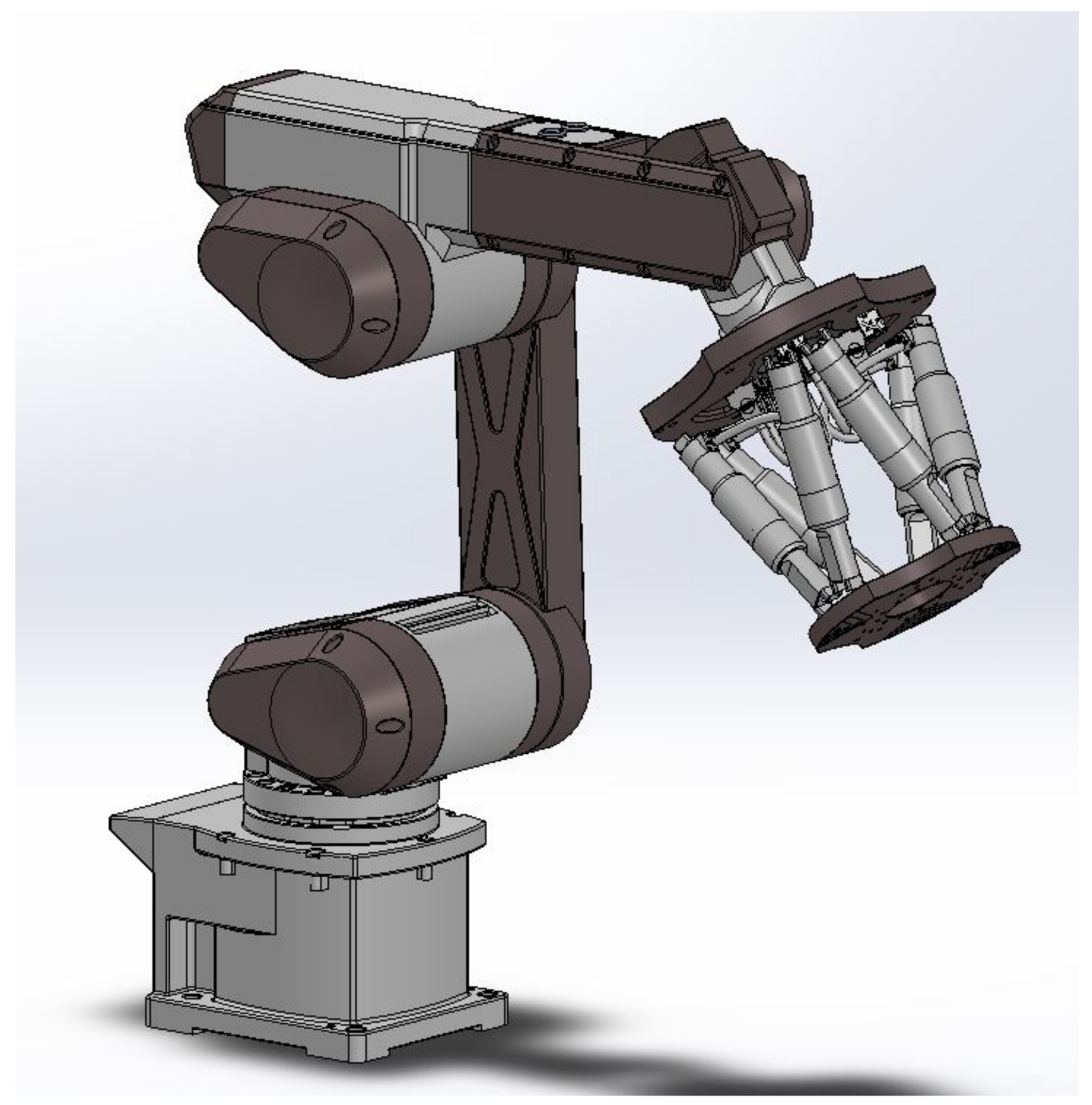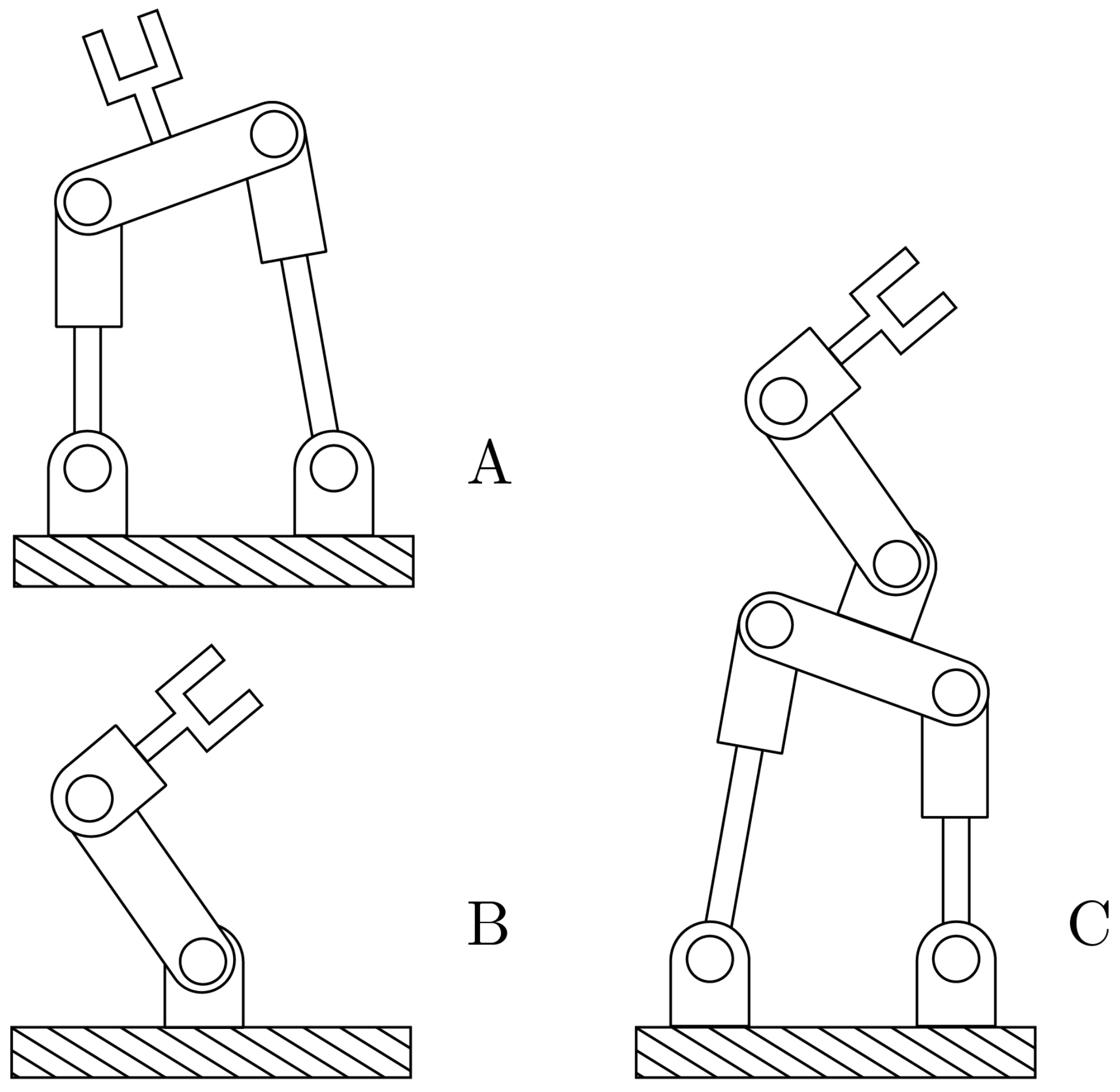Although the majority of the parallel mechanisms in the literature incorporate coincident passive joints in the form of universal or spherical joints at the top and bottom of a prismatic leg similar to the popular 6 DoF Stewart–Gough configuration [7,8], recent work has modified the design to use offset universal joints to increase stiffness and reduce manufacturing constraints [9]. This 6-RRRPRR parallel manipulator configuration with offset R-R joints, with individual parallel members constructed of rotary (R) and prismatic (P) joints listed in order, requires more general kinematic and calibration approaches than typically used with Stewart Platform designs due to the removal of the geometric simplifications permitted by the coincident passive joints and is of particular interest within this work. We present constraint-based approaches to solve the kinematics and calibration problems for strictly parallel manipulators and hybrid parallel-serial manipulators, such as the example pictured in Figure 1, with the general construction shown in Figure 2.

Parallel manipulators are advantageous with respect to physical properties of manipulator stiffness and deflection, but present significantly more challenges in analysis than serial manipulators due to the large number of kinematic parameters required to describe the manipulator and the large forward kinematic solution space [10]. Common planning operations, such as inverse and forward kinematics, are difficult to compute due to the possibility of singularities existing in the manipulator workspace, and the characteristic constraint-driven motion introduces difficulties in calibration. The calibration and kinematic evaluation of complex parallel manipulators typically relies on varying degrees of geometric simplifications and external measurements. Efficient forward kinematic calculation has been achieved through the use of special construction geometry, inverse-kinematic-residual minimization, algebraic solutions, and polynominal methods [11,12,13,14]. Hybrid manipulator kinematics encounter similar problems to strictly parallel manipulators, with closed-form solutions detailed for specific construction geometries such as stacked 3 DoF parallel manipulators [4].

Parallel manipulator calibration has been achieved using classic second-order constrained optimization techniques to simultaneously solve passive joint positions and kinematic parameters  [15]. Although similar methods are implemented for kinematic workspace analysis and design [16,17], the problem complexity grows rapidly with manipulator design. Subsequent calibration literature uses first-order fitting and addresses mechanism constraints by restricting physical motion of the manipulator [18,19], adding redundant joint instrumentation [20,21,22], or using inverse-kinematics solutions [23] and forward-kinematics solutions [24] to generate approximate passive joint information. Approaches that require manipulator modifications, such as physical motion restriction or joint instrumentation, are undesirable as they are difficult or impossible to add to existing manipulators. Accordingly, we focus on methods that approximate the passive joint information that can be extended to hybrid manipulators incorporating passive joint features.

The inverse-kinematic-residual approach to calibration minimizes the difference between a measured prismatic leg length and an estimate created from the inverse-kinematics solution at a desired pose [23]. This method can be described as a position-vector-minimization implementation of loop closure methods with the approximate passive joint information [20]. This calibration approach benefits from high-accuracy measurement methods, such as laser tracker metrology systems [25,26], and has been extended to solve the inverse-kinematics and calibrate a 6-RRRPRR parallel manipulator with offset R-R joints [3,27]. Recent work typically utilizes Product-of-Exponentials (POE) link representation [28], with successful calibrations demonstrated on a 3 DoF parallel manipulator and a 6 DoF Stewart Platform [29].

Pose-error Jacobian minimization methods based on forward-kinematics solutions are commonly used in serial manipulator calibrations in which an end-effector measurement is used to create a virtual closed kinematic chain [30]. The pose-error minimization embeds the passive joint estimate within the Jacobian to holistically minimize the difference between a measured pose and a forward-kinematics solution generated with the current parameter set. Analytical Jacobian formulations exist for standard Stewart Platform leg geometry [31], but not for general manipulators. The difficulty associated with determining analytical Jacobians has led to the use of computationally intensive and less accurate direct perturbation methods to find an approximate Jacobian [24,32] or the use of heuristic optimization methods to minimize pose-error such as the Nelder–Mead [33]. Recent work using pose-error minimization has focused on specialized manipulators with relatively low mechanical complexity. Mechanism-specific analytical Jacobians have been developed in 3 DoF [34] and 5 DoF [35] cases and implemented with regularization techniques and genetic algorithm fitting to allow for pose-error calibration.

Although standard Least-Squares fitting methods are common throughout literature, the noisy measurements have been identified as having large impacts on calibration quality due to low parameter identifiability [20]. Alternate approaches for handling the low parameter identifiability of parallel manipulators have been demonstrated in manipulator-specific or representation-specific cases, such as ridge regression, truncated singular value decomposition, and null space conditioning [36,37,38]. These techniques can positively impact the quality of the final calibration and have been compared in [29].

Post-calibration manipulator uncertainty analysis has been sparsely identified in the literature. Monte Carlo techniques have been implemented on parallel manipulator for analysis, but remain computationally expensive for comprehensive workspace analysis [39]. The uncertainty minimization calibration approach demonstrated by [21] utilizes a priori covariance estimates based on construction specifications for kinematic parameters and encoders as inputs. As the covariance estimates were inflated arbitrarily to maintain congruence with expected manufacturing tolerances, final pose uncertainty cannot reliably be obtained from this approach.

The manipulator-specific approach to model derivation and analysis found in state-of-the-art literature for parallel manipulators starkly contrasts with the mature body of work for general serial manipulators, and the common inverse-kinematic-residual minimization approaches are problematic to extend to holistic hybrid manipulator calibration. The myriad of possibilities for the construction of novel parallel and hybrid manipulators exacerbates the lack of consensus in the robotics field concerning their kinematics and calibration, driving the need for a simple and generalized representation capable of implementation across the variety of manipulators found in the industry and research sectors.

This paper’s contribution can be broken into three distinct areas. First, we present a general approach to describing any robotic manipulator with the same mathematical framework as serial-chain manipulators. Second, we provide general analytical methods to construct both kinematic and calibration Jacobians for any robot manipulator. Third, we leverage these methods to quantify the post-calibration pose uncertainty for any robot manipulator based on measurement uncertainty, which has not been previously done. This work extends the state-of-the-art by allowing parallel, hybrid, and serial manipulators to be analyzed, calibrated, and controlled with the same analytical tools.

This paper is structured as follows. In Section 2, we review the nonlinear least squares based kinematic calibration framework as implemented on serial robots and detail how a parallel manipulator can be represented using serial parameterization and simplified numerical kinematics solutions. A method to enforce mechanical constraints on a Jacobian level via null-space is introduced as a component of the inverse kinematics method. The analytical velocity Jacobian for a parallel manipulator is presented. We then extend the constraint propagation to generate a unified calibration Jacobian for hybrid manipulators allowing for simultaneous calibration. We additionally present a detailed uncertainty analysis based on this calibration method and develop guidelines for uncertainty-aware calibrations. In Section 3, we demonstrate this method on a simulated and real world hybrid manipulator, respectively. In Section 4, we discuss calibration performance and possible extensions of our work. For convenience, the notion used throughout this paper is summarized in

Table 1. Mathematical Notation Summary.

Symbol	Description
$\mathbf{R}$	[3 × 3] Rotation matrix
$\mathbf{d}$	[3 × 1] Cartesian displacement vector
$\mathbf{T}$	[4 × 4] Homogeneous transformation matrix
$\mathbf{\tau }$	Vector-based transform parameterization
$\mathbf{e}$	Pose-error vector
$\mathbf{J}$	Calibration Jacobian
$\mathcal{C}$	Constraint Jacobian
$\varphi$	Vector of all kinematic parameters
$\theta$	Vector of all actuator inputs
$\psi$	Vector of all passive joints
v	Subscript denoting velocity Jacobian
N	Number of measurement poses within a data set
P	Number of $\varphi$ terms for a link
L	Number of links representing a manipulator

. Matrix size is displayed in brackets before description and subscripts provide contextual definitions.

2. Materials and Methods

2.1. Calibration Methodology Overview

We develop general pose-error Jacobians for kinematics and calibration by applying existing serial manipulator link definitions and Jacobian formulations to individual kinematic chains between the distal and proximal frames of a parallel manipulator. By segregating the Jacobian information related to active joints, passive joints, and kinematic parameters, we construct constraint matrices between all kinematic chains within the manipulator. We condition the pose-error Jacobians with the null space of these constraint matrices to only permit updates that do not introduce error between the distal frames of each kinematic chain. This produces a single Jacobian for the entire parallel manipulator, permitting it to be used for fitted kinematic and calibration solutions.

The calibration approach in this section is described in a general manner. Analytical definitions of pose-error Jacobians exist for many serial robotic link representations, and are straightforward to calculate if not available. The advantages of individual parameterizations vary and are dependent on the final application.

2.2. Pose-Error Minimization Framework

Calibration procedures aim to reduce discrepancies in expected and measured poses for a robot manipulator. We extend an established calibration framework that minimizes a 6 DoF pose-error calculated at a number of measured poses by adjusting the nominal kinematic model parameters of a manipulator [30]. We detail the basic principles and operation of this framework to provide contextual basis for our extensions starting in Section 2.3.

2.2.1. Objective and Error Formulation

Calibration can be expressed as the general optimization problem

$$\underset{\varphi }{argmin}{\parallel \mathbf{E}\parallel }^2,$$

(1)

where $\mathbf{E}$ is a general representation of a pose-error vector at all points within a measurement data set. A robust error model is required to evaluate the performance of the kinematic model and permit effective calibration. The position error $\Delta \mathbf{p}$ is calculated as

$$\Delta \mathbf{p}={\mathbf{d}}_{\mathrm{m}}-{\mathbf{d}}_{\mathrm{c}},$$

(2)

where $\mathbf{d}$ represents a vector containing the Cartesian position of the robot manipulator end-effector with subscript denoting as the value being either obtained through a measurement (m) or calculation (c) via the mathematical model.

Small rotational errors can be represented as a differential orthogonal rotation [30], however, this approach poorly represents large rotational errors. To provide more robust calibration behavior, we implement an angle-axis based alternative that linearizes the rotation error for all error magnitudes as

$$\begin{array}{cc}\hfill e^{{[\Delta \Omega ]}_{\times }}={\mathbf{R}}_{\mathrm{e}}& ={\mathbf{R}}_{\mathrm{m}}{\mathbf{R}}_{\mathrm{c}}^{\top },\hfill \end{array}$$

(3)

where $\mathbf{R}$ represents the rotation matrix representation of the robot manipulator end-effector using the subscript notation defined above. The angle-axis equivalent $\Delta \Omega$ is calculated from the rotation error (${\mathbf{R}}_e$) using standard conversion methods [40].

These error components are packed into a pose-error vector as

$$\mathbf{e}=\left[\begin{array}{c}\Delta \mathbf{p}\\ \Delta \Omega \end{array}\right],$$

(4)

where $\Delta \mathbf{p}$ is the position error and $\Delta \Omega$ is the rotation error. The calculation of this error vector between transforms is referenced in this work as $\mathbf{e}\left({\mathbf{T}}_1,{\mathbf{T}}_2\right)$, although the inputs are typically contextually inferred.

2.2.2. Jacobian Packing

Pose-error evolution with respect to the manipulator kinematic parameters $\mathbf{\varphi }$ is described in a linear manner by analytical Jacobians. When evaluated at a pose with known actuator positions $\mathbf{\theta }$, each calibrated parameter produces a [6 × 1] vector of the relationship between the 6 DoF error term and perturbations to the respective kinematic parameter. As a single error term exists for each measured pose, the vectors corresponding to all kinematic parameters are horizontally concatenated in a common Jacobian packing method [30]. For convenience, parameters associated with an individual serial link are grouped, resulting in the block Jacobian for a single pose of

$${\mathbf{J}}_{\varphi }=\left[\underset{\mathrm{Link}1}{\underbrace{\left[\frac{\partial \mathbf{e}}{\partial {\varphi }_{1,1}}\cdots \frac{\partial \mathbf{e}}{\partial {\varphi }_{\mathit{1},\mathit{P}}}\right]}}\cdots \underset{\mathrm{Link}\mathrm{L}}{\underbrace{\left[\frac{\partial \mathbf{e}}{\partial {\varphi }_{L,1}}\cdots \frac{\partial \mathbf{e}}{\partial {\varphi }_{\mathit{L},\mathit{P}}}\right]}}\right],$$

(5)

where the Jacobian blocks corresponding to links with P parameters are displayed. Blocks corresponding to any number of links can be concatenated to permit calibration of any possible serial manipulator construction. Symbolic definitions for pose-error Jacobian components for the link parameterizations used within this work are provided in Appendix B.

Multiple pose measurements are required for convergence of the pose-error minimization solution during calibration of nontrivial robotic manipulators. To accommodate any number of measurements, pose-error terms (4) and the concatenated kinematic parameter Jacobian (5) are vertically concatenated for N points as

$${\mathbf{J}}_{\Phi }=\left[\begin{array}{c}{\mathbf{J}}_{\mathbf{\varphi },1}\\ {\mathbf{J}}_{\mathbf{\varphi },2}\\ ⋮\\ {\mathbf{J}}_{\mathbf{\varphi },N}\end{array}\right],\mathbf{E}=\left[\begin{array}{c}{\mathbf{e}}_1\\ {\mathbf{e}}_2\\ ⋮\\ {\mathbf{e}}_N\end{array}\right].$$

(6)

Here, a Jacobian representing all measured poses is expressed with an uppercase $\Phi$, while a Jacobian representing any single measured pose is expressed with a lowercase $\varphi$.

2.2.3. Parameter Update

Manipulator kinematic parameters $\varphi$ can be found to minimize the pose-error using the Gauss–Newton approach to nonlinear least squares with ${\mathbf{J}}_{\Phi }$ and $\mathbf{E}$. Successive $\Delta \varphi$ steps on a set of all measured poses are calculated as

$$\Delta \varphi ={\mathbf{J}}_{\Phi }^{†}\mathbf{E},$$

(7)

where † indicates the pseudoinverse of a matrix. Within this work, the pseudoinverse is calculated using Singular Value Decomposition (SVD) of the Jacobian matrix as

$${\mathbf{A}}^{†}=\mathbf{V}{\Sigma }^{-1}{\mathbf{U}}^{\top },$$

(8)

where $\mathbf{U},\Sigma ,\mathbf{V}$ are standard SVD components [41]. Small singular values within $\Sigma$ corresponding to poorly identifiable kinematic parameters can result in the calculation of extremely large terms within the pseudoinverse generation process. These parameters are ignored by replacing the terms within ${\Sigma }^{-1}$ that correspond with singular values with condition numbers above a specified threshold with 0 [42]. This produces a similar step to Levenberg–Marquardt fitting with a fixed damping parameter.

The step is added to the existing $\varphi$ and the process is repeated until convergence conditions are met. More robust stepping algorithms such as the Levenberg–Marquardt method [43] or Sequential Quadratic Programming [44] can also be used to generate steps in cases where high parameter sensitivity results in nonconvergent behavior for standard Gauss–Newton steps, but implementation details for these algorithms is outside of the scope of this work and may require additional gradients to be developed. The constrained Jacobians produced in this work are applied for a variety of analytical purposes outside of fitting techniques, and are a primary focus of this work.

2.3. Parallel Manipulator Parameterization and Kinematics

To calibrate parallel manipulators simultaneously with serial links within the framework detailed above, an analogous Jacobian is required that captures the sensitivities of the kinematic parameters of the manipulator with respect to the final pose. A parallel manipulator is represented as a special serial link which returns a single transform provided a set of active joint inputs, with kinematic behavior mathematically represented by standard serial links.

Actively controlled joint parameters corresponding to the linear or rotary actuators of a robotic manipulator are denoted by $\mathbf{\theta }$, while passively driven joint parameters such as unpowered bearings or slides driven by the constraints of the manipulator are denoted by $\mathbf{\psi }$. Static offsets that describe the manipulator (for example mechanical linkages and metrology systems used during calibration) are incorporated in this work with general symbol $\tau$, which represents a parameterized transform in vector format that can be calibrated as a typical link within the presented framework.

2.3.1. Serial Chain Parameterization

Parallel manipulators are constructed from several serial chains connected in a manner that constrains their motion. These serial chains, termed parallel members within this work, are often underactuated due to the presence of one or more unpowered joints. A parallel member is represented using a standard serial link models positioned by pose offsets $\tau$ to align the distal and proximal frames of the complete parallel manipulator in the home position. Shown with appropriate notation in Figure 3, each parallel member $\mathbf{M}$ can have any number of links. Individual serial links within the parallel member serial chains are denoted as $M_{j,k}$, in which the first subscript denotes the parent parallel member and the second the relative position of the link within the parallel member.

The pose of a hybrid manipulator can be described by constructing a serial chain $\mathbf{P}$ composed of any one parallel member and the strictly serial links of the manipulator. In each possible serial chain, the distal and proximal ends of the parallel member as well as the complete hybrid manipulator must remain coincident in any valid configuration as displayed in Figure 3. These frame constraints are used to capture the sensitivities of the complete manipulator and allow for calibration.

2.3.2. Forward Kinematics

The constraints that drive the passive joints of a parallel manipulator introduce additional nonlinearities into the forward kinematics problem, resulting in numerous valid analytical solutions for any set of input $\mathbf{\theta }$ [45]. We avoid the complexity of analytical solutions by implementing a nonlinear least squares inverse kinematics fitting method with the serial chain representation of the parallel manipulator to generate a valid transform for a parallel manipulator. This method allows a single valid solution within the desired workspace to be found quickly in cases with a singularity-free work envelope and a nearby pose approximation. Collision checking for fitted solutions can be conducted quickly due to the proximity to the initial feasible pose.

The forward kinematics fitting process adjusts pose estimate vector $\mathbf{\tau }$, corresponding to ${\mathbf{T}}_{\mathrm{parallel}}$ in Figure 3, and passive joint parameters $\psi$ to yield a valid final transform for the parallel manipulator. This process can be expressed as the optimization problem for the M parallel members as

$$\begin{array}{cc}\hfill \underset{\tau ,\psi }{argmin}& \parallel {\mathbf{E}}_{\mathrm{f}}{\parallel }^2\hfill \\ \hfill \mathrm{subject}\mathrm{to}& \mathbf{e}\left({\mathbf{T}}_1,{\mathbf{T}}_m\right)=0\forall m\in \mathbf{M},\hfill \end{array}$$

(9)

where each $\mathbf{T}$ is the transform calculated for an individual parallel member indicated via subscript with associated input set $\left(\mathbf{\varphi },\mathbf{\theta },\mathbf{\psi }\right)$. Without loss of generality, we choose a point and quaternion ($\mathbf{p}\&\mathbf{q}$) formulation of pose to generate singularity-free Jacobians over a small number of parameters. Pose-error terms (4), between the distal transform of each parallel member at $\mathbf{\psi }$ and the pose guess $\mathbf{\tau }$, are minimized to find a convergent forward kinematics solution. The errors for each of the M parallel members of the manipulator are vertically concatenated similar to (6) into a single [6$M\times$1] error vector as

$${\mathbf{E}}_{\mathrm{f}}=\left[\begin{array}{c}{\mathbf{e}}_1\\ {\mathbf{e}}_2\\ ⋮\\ {\mathbf{e}}_M\end{array}\right].$$

(10)

The forward kinematic error ${\mathbf{E}}_{\mathrm{f}}$ is minimized by constructing Jacobian ${\mathbf{J}}_{\mathrm{f}}$ to adjust both pose estimate and passive joint parameters simultaneously as

$${\mathbf{J}}_{\mathrm{f}}=\left[\begin{array}{cccc}{\mathbf{J}}_{\tau }& {\mathbf{J}}_{\psi ,1}& \cdots & \mathbf{0}\\ ⋮& ⋮& \ddots & ⋮\\ {\mathbf{J}}_{\tau }& \mathbf{0}& \cdots & {\mathbf{J}}_{\psi ,M}\end{array}\right],$$

(11)

where ${\mathbf{J}}_{\tau }$ used in this work is provided in Appendix A and ${\mathbf{J}}_{\psi }$ are the horizontally concatenated serial chain velocity Jacobians for the passive joints of the parallel members identified by the second subscript. As active joint values $\theta$ are fixed for any given forward kinematics problem, the velocity Jacobian ${\mathbf{J}}_{\theta }$ terms are not included. Kinematic parameters $\mathbf{\varphi }$ are used to generate the error terms, but are absent from this Jacobian formulation as they are not adjusted in this process.

The update step for the fitting process is calculated similarly to (7) as

$$\left[\begin{array}{c}\Delta \mathbf{\tau }\\ \Delta \psi \end{array}\right]={\mathbf{J}}_{\mathrm{f}}^{†}{\mathbf{E}}_{\mathrm{f}}.$$

(12)

The forward kinematics fitting process terminates when error is reduced below a specified threshold or updates are no longer reducing error by a secondary threshold. To ensure convergence to the expected pose, it is preferable to use a more accurate initial estimate for $\mathbf{\tau }$ based on nominal inputs or metrology measurements.

2.3.3. Inverse Kinematics

Determining the active joint parameters $\mathbf{\theta }$ to reach a specific pose is necessary for motion planning. We extend the inverse kinematics fitting methods developed in the previous section to formulate a constrained velocity Jacobian that describes a linear relationship between active and passive joint angles and end-effector pose. This allows valid input combinations close to the starting position of the manipulator for a desired pose to be found with nonlinear least squares methods.

The passive joint parameters $\psi$ of a parallel manipulator are required to fully characterize its motion. Provided a valid starting configuration for the parallel manipulator and a desired pose ${\mathbf{T}}_{\mathrm{des}}$, an identical pose-error $\mathbf{e}$ is calculated using (4) for each parallel member. The inverse kinematics fitting process is formulated as

$$\begin{array}{cc}\hfill \underset{\theta ,\psi }{argmin}& \parallel \mathbf{e}\left({\mathbf{T}}_{\mathrm{des}},{\mathbf{T}}_{\mathrm{parallel}}\right){\parallel }^2\hfill \\ \hfill \mathrm{subject}\mathrm{to}& \mathbf{e}\left({\mathbf{T}}_1,{\mathbf{T}}_m\right)=0\forall m\in \mathbf{M},\hfill \end{array}$$

(13)

where both active and passive joint values are adjusted to reach the desired pose. A valid starting configuration indicates that the distal frames of all constituent parallel members are coincident as displayed by ${\mathbf{T}}_{\mathrm{parallel}}$ in Figure 3.

At a coincident configuration the difference in parallel member final pose (10) must be zero, allowing for the relationship between parallel member parameter changes and coincident frame motion to be modelled. The pose estimate Jacobian (11) is reframed as a constraint to maintain a coincident frame and expanded to incorporate the active joints of the parallel member $\theta$ as

$$\mathcal{C}=\left[\begin{array}{ccccccc}{\mathbf{J}}_{\tau }& -{\mathbf{J}}_{\theta ,1}& \cdots & \mathbf{0}& -{\mathbf{J}}_{\psi ,1}& \cdots & \mathbf{0}\\ ⋮& ⋮& \ddots & ⋮& ⋮& \ddots & ⋮\\ {\mathbf{J}}_{\tau }& \mathbf{0}& \cdots & -{\mathbf{J}}_{\theta ,M}& \mathbf{0}& \cdots & -{\mathbf{J}}_{\psi ,M}\end{array}\right].$$

(14)

To yield a valid coincident pose for the parallel manipulator for a parameter update step (7), it must have form

$$\mathcal{C}\left[\begin{array}{c}\Delta \mathbf{\tau }\\ \Delta \theta \\ \Delta \psi \end{array}\right]=\mathbf{0},$$

(15)

which can also be expressed as,

$$M\Delta {\mathbf{J}}_{\tau }\mathbf{\tau }={\mathbf{J}}_{\theta }\Delta \theta +{\mathbf{J}}_{\psi }\Delta \psi ,$$

(16)

where ${\mathbf{J}}_{\theta }$ and ${\mathbf{J}}_{\psi }$ are the horizontally concatenated Jacobian blocks of M parallel members.

Any change in the coincident frame pose representation $\mathbf{\tau }$ directly impacts the total pose-error of the parallel manipulator as defined in (4) to an arbitrary frame of interest as

$$\Delta \mathbf{e}={\mathbf{J}}_{\tau }\Delta \mathbf{\tau }.$$

(17)

By substitution and matrix manipulation,

$$\Delta \mathbf{e}=\frac{1}{M}\left[\begin{array}{cc}{\mathbf{J}}_{\theta }& {\mathbf{J}}_{\psi }\end{array}\right]\left[\begin{array}{c}\Delta \theta \\ \Delta \psi \end{array}\right],$$

(18)

where it becomes apparent that a scaling factor of $\frac{1}{M}$ is necessary to condition the parallel member Jacobians for use in a constrained parallel manipulator.

Nota Bene: this approximation is only valid in cases where the parallel manipulator begins in a constrained state with zero constraint error and does not inherently enforce the constraint with an arbitrary parameter step. The addition of this scaling factor only ensures that the weighting found during the forward kinematics process is expressed during the calibration process, removing the need to generate a specific $\mathbf{\tau }$ constraint.

The relationship (18) is used in the inverse kinematic fitting process. By considering the active and passive joints of each parallel member of a parallel manipulator separately, a composite velocity Jacobian for independent parallel member motion is defined as

$${\mathbf{J}}_{\mathrm{v}}=\frac{1}{M}\left[\begin{array}{cc}{\mathbf{J}}_{\theta }& {\mathbf{J}}_{\psi }\end{array}\right],$$

(19)

where M represents the number of parallel members that define a parallel manipulator and ${\mathbf{J}}_{\theta }$ and ${\mathbf{J}}_{\psi }$ are the active and passive joint parameter Jacobians of all constituent parallel members concatenated in the link-wise manner described in (5).

While representing the motion of many separate serial chains, the ${\mathbf{J}}_{\mathrm{v}}$ in (19) does not yet capture the constraints of the complete parallel manipulator as each chain can move without impacting the others. For any valid pose, the end-effector frames for each of the parallel members serial chains must remain coincident; no pose-error can exist between them. This constraint is enforced by using the previously calculated Jacobians ${\mathbf{J}}_{\theta }$ and ${\mathbf{J}}_{\psi }$. To match the column order of (19), the constraint matrix for each Jacobian is constructed separately but with identical block structure. The constraint matrix associated with ${\mathbf{J}}_{\theta }$ is

$${\mathcal{C}}_{\theta }=\left[\begin{array}{ccccc}{\mathbf{J}}_{\theta ,1}& -{\mathbf{J}}_{\theta ,2}& \mathbf{0}& \cdots & \mathbf{0}\\ {\mathbf{J}}_{\theta ,1}& \mathbf{0}& -{\mathbf{J}}_{\theta ,3}& \cdots & \mathbf{0}\\ ⋮& ⋮& ⋮& \ddots & ⋮\\ {\mathbf{J}}_{\theta ,1}& \mathbf{0}& \mathbf{0}& \cdots & -{\mathbf{J}}_{\theta ,M}\end{array}\right],$$

(20)

where the second Jacobian subscript identifies the parallel member each block is associated with. The passive joint parameter constraint matrix ${\mathcal{C}}_{\psi }$ is generated by substituting the appropriate ${\mathbf{J}}_{\psi }$ components for the parallel members into the structure. The individual constraint matrices are combined for final use as

$${\mathcal{C}}_{\mathrm{v}}=\left[\begin{array}{cc}{\mathcal{C}}_{\theta }& {\mathcal{C}}_{\psi }\end{array}\right],$$

(21)

where the column dimension matches that of ${\mathbf{J}}_{\mathrm{v}}$.

To ensure that no constraint error is generated by updates to $\theta$ and $\psi$, a null space is constructed from the combined constraint matrix and propagated to the combined parallel manipulator velocity Jacobian ${\mathbf{J}}_{\mathrm{v}}$ as

$${\mathbf{J}}_{\mathrm{v}|\mathcal{C}}^{†}=\mathcal{N}\left({\mathcal{C}}_{\mathrm{v}}\right){\left({\mathbf{J}}_{\mathrm{v}}\mathcal{N}\left({\mathcal{C}}_{\mathrm{v}}\right)\right)}^{†},$$

(22)

where $\mathcal{N}\left({\mathcal{C}}_{\mathrm{v}}\right)$ indicates the null space of the input constraint matrix. It should be noted that the null space of a matrix is not unique - any valid null space can be multiplied by a real value to yield another valid solution [46]. The construction of (22) can use any valid null space.

For use in the inverse kinematics of hybrid manipulators, this must be converted via a second pseudo-inverse operation to standard form ${\mathbf{J}}_{\mathrm{v}|\mathcal{C}}$ or calculated in the alternate form

$${\mathbf{J}}_{\mathrm{v}|\mathcal{C}}=\left({\mathbf{J}}_{\mathrm{v}}\mathcal{N}\left({\mathcal{C}}_{\mathrm{v}}\right)\right)\mathcal{N}{\left({\mathcal{C}}_{\mathrm{v}}\right)}^{†}.$$

(23)

The constrained velocity Jacobian is used to successively calculate parameter steps as shown in (7), with the process terminating once ${\parallel \mathbf{E}\parallel }^2$ has fallen below a set tolerance or additional exit conditions are met. If the fitting process fails to converge, the feasibility of the pose should be evaluated. As passive joints are updated during every forward kinematic calculation, components of the constrained velocity Jacobian related to $\psi$ are removed before step calculation, leaving only the desired $\theta$ components.

2.4. Parallel Manipulator Calibration

The constraint methods implemented for inverse kinematic calculations of parallel manipulators can be used to create a pose-error Jacobian for calibrated kinematic parameters. By imposing kinematic constraints to each of the parallel members of a manipulator, we assemble complete parameterized kinematic information and condition it such that the parallel manipulator acts as a virtual serial link in hybrid manipulator cases.

2.4.1. Jacobian Packing

The passive joints of a parallel manipulator are responsible for the characteristic closed-loop kinematics but are seldom fitted with encoders in commercial units. Should the joint angles of one parallel members be completely known, the calibration problem can be solved by a standard serial approach as implemented in [21]. To remove the need for fitting a platform with additional encoders, our work considers these passive joints as an additional set of unknown parameters to be solved for on a pose-by-pose basis. The Jacobians linked to kinematic parameter and passive joints are emplaced into a composite calibration Jacobian ${\mathbf{J}}_{\mathrm{cal}}$ as

$${\mathbf{J}}_{\mathrm{cal}}=\left[\begin{array}{cccccc}{\mathbf{J}}_{\varphi ,1}& {\mathbf{J}}_{\psi ,1}& \mathbf{0}& \cdots & & \mathbf{0}\\ {\mathbf{J}}_{\varphi ,2}& \mathbf{0}& {\mathbf{J}}_{\psi ,2}& \cdots & & \mathbf{0}\\ ⋮& ⋮& ⋮& \ddots & ⋮& ⋮\\ {\mathbf{J}}_{\varphi ,N}& \mathbf{0}& \mathbf{0}& \cdots & & {\mathbf{J}}_{\psi ,N}\end{array}\right],$$

(24)

where the second subscript identifies the pose to which the Jacobian is related. Kinematic parameters associated with the standard serial links are separated from those associated with each parallel members and recombined as

$${\mathbf{J}}_{\varphi ,i}=\left[\begin{array}{cc}{\mathbf{J}}_{\varphi ,\mathrm{serial}}& {\mathbf{J}}_{\varphi ,\mathrm{parallel}}\end{array}\right].$$

(25)

2.4.2. Constraint Matrix Construction

The calibration Jacobian matrix ${\mathbf{J}}_{\mathrm{cal}}$ captures the kinematics of each serial chain within the hybrid robotic manipulator, but ignores the physical constraints that drive the passive joints within the manipulator. Each of the individual parallel members within the parallel manipulator share distal and proximal frames; zero pose-error (4) exists between any constituent serial chain at any valid set of joint parameters $\mathbf{\theta }$ and $\mathbf{\psi }$. Any kinematic parameter $\mathbf{\varphi }$ changes made during calibration must not violate this zero pose-error constraint. By conditioning ${\mathbf{J}}_{\mathrm{cal}}$ with the null space of linearized kinematic parameter constraints ${\mathcal{C}}_{\varphi }$ and passive joint constraints ${\mathcal{C}}_{\psi }$, valid parameter steps are enforced.

The format presented in (20) is implemented as to calculate ${\mathcal{C}}_{\varphi }$ and ${\mathcal{C}}_{\psi }$ for N pose measurements. These component constraint matrices are packed into a composite matrix in a manner similar to (24) with structure

$${\mathcal{C}}_{\mathrm{cal}}=\left[\begin{array}{cccccc}\mathbf{0}& {\mathcal{C}}_{\varphi ,1}& {\mathcal{C}}_{\psi ,1}& \mathbf{0}& \cdots & \mathbf{0}\\ \mathbf{0}& {\mathcal{C}}_{\varphi ,2}& \mathbf{0}& {\mathcal{C}}_{\psi ,2}& \cdots & \mathbf{0}\\ ⋮& ⋮& ⋮& \ddots & ⋮\\ \mathbf{0}& {\mathcal{C}}_{\varphi ,N}& \mathbf{0}& \mathbf{0}& \cdots & {\mathcal{C}}_{\psi ,N}\end{array}\right],$$

(26)

where the subscripted number indicates the pose with which each Jacobian is associated with. As the serial link kinematic parameters cannot cause error between the parallel members end frames, zeros matrices corresponding to the columns of these parameters are appended to the left hand side of the matrix to match the dimensionality of the standard serial link Jacobians present in (24).

When used with hybrid robotic manipulators, the Jacobians used to generate the constraint matrices must represent the error evolution of the distal frames of the parallel members that compose a parallel manipulator rather than that of the hybrid manipulator. Should multiple parallel manipulators be present in the hybrid manipulator, additional sets of constraints are required.

Similarly to the inverse kinematics case, the constrained pseudo-inverse is calculated as

$${\mathbf{J}}_{\mathrm{cal}|\mathcal{C}}^{†}=\mathcal{N}\left({\mathcal{C}}_{\mathrm{cal}}\right){\left({\mathbf{J}}_{\mathrm{cal}}\mathcal{N}\left({\mathcal{C}}_{\mathrm{cal}}\right)\right)}^{†}.$$

(27)

While it is necessary to incorporate the passive joint parameters and associated constraints to properly capture the dynamics of a parallel manipulator, the forward kinematics process (Section 2.3.2) must be run to acquire updated pose information at the beginning of each calibration loop. To prevent redundant parameter updates, the portions of the pseudoinverse related to these passive $\psi$ parameters are removed as

$${\mathbf{J}}_{\Phi |\mathcal{C}}^{†}=\left[\mathbf{I}\mathbf{0}\right]{\mathbf{J}}_{\mathrm{cal}|\mathcal{C}}^{†},$$

(28)

where $\mathbf{I}$ is a full-rank identity matrix appropriately sized to match the number of $\varphi$ terms and zeros are appended to reach proper matrix dimensions. In the case where the Jacobian for a single measured pose is generated, notation ${\mathbf{J}}_{\varphi |\mathcal{C}}$ is used. Using the reduced Jacobian form a calibration step is calculated according to (7) and added to the parameter estimate from the previous step.

2.4.3. Pose-by-Pose Jacobian Generation

In the case of D DoF data collection, the dimensions of the ${\mathbf{J}}_{\mathrm{cal}}$ and the associated ${\mathcal{C}}_{\mathrm{cal}}$ are defined as

$$[DMN\times \left(\mathrm{length}\left(\mathbf{\varphi }\right)+U\mathrm{length}\left(\mathbf{\psi }\right)\right)],$$

(29)

where N is the total number of measured poses and U is the number of parallel manipulator poses requiring a unique $\mathbf{\psi }$ solution. For purely random pose selection $N=U$, and the linear growth of the system dictates that $DM>\mathrm{length}\left(\mathbf{\psi }\right)$ for the problem to remain defined with a sufficiently large number of pose measurements. If this condition does not exist, multiple pose measurements must be collected for each $\mathbf{\psi }$ solution by retaining the parallel manipulator pose while moving the strictly serial links such that $N>U$. The column of shared kinematic parameters $\varphi$ of the strictly serial links results in a linked constraint matrix that does not permit direct simplification, demanding computationally expensive null space and pseudoinverse calculations for (27).

To permit the problem to remain computationally tractable for general calibration purposes, we present a method for enforcing the constraint framework on a pose-by-pose basis. Efficient Jacobian generation is accomplished by isolating the parallel manipulators of a hybrid manipulator and analyzing them individually. Serial Jacobians for kinematic parameters $\varphi$ and passive joints $\psi$ are generated for each of the M parallel members and horizontally concatenated to form composite Jacobians ${\mathbf{J}}_{\varphi }$ and ${\mathbf{J}}_{\psi }$. All Jacobians generated during this process only consider the parallel manipulator-values are relative to the proximal frame of the parallel manipulator. These Jacobians are then combined to form unconstrained calibration Jacobian

$${\tilde{\mathbf{J}}}_{\mathrm{cal}}=\frac{1}{M}\left[\begin{array}{cc}{\mathbf{J}}_{\varphi }& {\mathbf{J}}_{\psi }\end{array}\right].$$

(30)

The constraint Jacobians are constructed in the manner proposed in (20) as

$${\tilde{\mathcal{C}}}_{\mathrm{cal}}=\left[\begin{array}{cc}{\mathcal{C}}_{\varphi }& {\mathcal{C}}_{\psi }\end{array}\right].$$

(31)

The existence of a valid solution for passive joints is required to be present at the time of Jacobian generation. These solutions are generated during each epoch of the calibration process using the forward kinematics approach, and splits the fitting problem to allow for faster operation.

Unlike the prior solution approach, the constraint must be applied in a manner that yields a constrained Jacobian rather than the pseudoinverse calculated in (27) and (28) as

$${\tilde{\mathbf{J}}}_{\varphi |\mathcal{C}}={\tilde{\mathbf{J}}}_{\mathrm{cal}}\mathcal{N}\left({\tilde{\mathcal{C}}}_{\mathrm{cal}}\right){\left(\left[\mathbf{I}\mathbf{0}\right]\mathcal{N}\left({\tilde{\mathcal{C}}}_{\mathrm{cal}}\right)\right)}^{†},$$

(32)

where $\mathbf{I}$ is a full-rank identity matrix appropriately sized to match the number of $\varphi$ terms and zeros are appended to reach proper matrix dimensions.

The Jacobian ${\tilde{\mathbf{J}}}_{\varphi |\mathcal{C}}$ generated in this manner is in the parallel manipulator local frame and must be transformed to reflect the geometric position of the manipulator within the hybrid manipulator before use [47]. As implemented, this process transforms the Jacobian with rows corresponding to position and rotation error terms (4) as

$$\mathbf{J}=\left[\begin{array}{c}{\mathbf{J}}_{\mathbf{p}}\\ {\mathbf{J}}_{\Omega }\end{array}\right]$$

(33)

to desired world frame, designated as frame 0 within this work, from local proximal and distal frames $\ell -1$ and ℓ as

$${\mathbf{J}}_{\mathrm{world}}=\left[\begin{array}{cc}{}^0{\mathbf{R}}_{\ell }& \mathbf{0}\\ \mathbf{0}& {}^0{\mathbf{R}}_{\ell }\end{array}\right]\left[\begin{array}{c}{\mathbf{J}}_{\mathbf{p}}-{\left[{}^{\ell }{\mathbf{d}}_{\ell \to L}\right]}_{\times }{\mathbf{J}}_{\Omega }\\ {\mathbf{J}}_{\Omega }\end{array}\right],$$

(34)

where the associated rotation matrices $\mathbf{R}$ and position offsets $\mathbf{p}$ are calculated using the other links of the hybrid manipulator.

The Jacobians for each constituent link in the manipulator are horizontally concatenated to yield the final calibration Jacobian. This process, although appearing to be a minor alteration to the methods described in Section 2.4 ensures that constrained calibration can be accomplished with sufficiently large pose data sets on manipulators with large numbers of passive joints that require fitting by reducing Jacobian dimensions to

$$[DN\times \mathrm{length}\left(\mathbf{\varphi }\right)].$$

(35)

The Jacobians generated in this manner have been validated to match those generated using numerical parameter perturbation methods.

2.5. Pose Uncertainty Estimation

A major contribution of this work is extending the constrained Jacobians described in this work to estimate the pose uncertainty of a calibrated robotic manipulator. We detail the process for propagating covariance matrix representations of known measurement uncertainty in the pose-error (4) space and manipulator encoder resolutions at any pose. This is of particular interest in model-based positioning control cases with high accuracy requirements.

Residual pose uncertainty after a calibration is driven in part by measurements with uncertainty being incorporated into the least-squares fitting process. The measurement uncertainties are propagated into the final fitted parameters via the developed calibration Jacobians (28) as

$$\begin{array}{cc}\hfill {\Sigma }_{\varphi }& ={\mathbf{J}}_{\Phi |\mathcal{C}}^{†}{\Sigma }_p{\left({\mathbf{J}}_{\Phi |\mathcal{C}}^{†}\right)}^{\top },\hfill \end{array}$$

(36)

where ${\Sigma }_{\varphi }$ is the covariance matrix for the calibrated kinematic parameters $\varphi$ arranged to match the column order of ${\mathbf{J}}_{\mathrm{cal}|\mathcal{C}}$. The covariance matrix ${\Sigma }_p$ is constructed by diagonally inserting the covariance matrices for all pose measurements used in the calibration diagonally as

$${\Sigma }_p=\left[\begin{array}{ccc}{\Sigma }_{p,1}& & \mathbf{0}\\ & \ddots & \\ \mathbf{0}& & {\Sigma }_{p,N}\end{array}\right],$$

(37)

where ${\Sigma }_{p,n}$ indicates the (DoF × DoF) covariance matrix associated with an individual pose measurement. In this work, pose covariance matrix is (6 × 6), with elements ordered to match the pose-error vector (4) as $[{\mathbf{p}}_{\mathrm{x}},{\mathbf{p}}_{\mathrm{y}},{\mathbf{p}}_{\mathrm{z}},{\Omega }_{\mathrm{x}},{\Omega }_{\mathrm{y}},{\Omega }_{\mathrm{z}}]$. Each of these components is expressed in the units of $m^2$ and $ra{d}^2$ for position and rotation error terms, respectively.

Parameter uncertainty information is extended back into error space for measured poses using covariance propagation techniques [41] with general form

$$\begin{array}{cc}\hfill {\Sigma }_b& =\mathbf{J}{\Sigma }_a{\mathbf{J}}^{\top },\hfill \end{array}$$

(38)

where $\mathbf{J}=\frac{\partial \mathbf{a}}{\partial \mathbf{b}}$. Pose-error uncertainty is also influenced by the use of digital encoders for joint measurement purposes, as there exists a degree of uncertainty in the final positions of any joint parameter when measured in discrete intervals. The motion of the manipulator due to these variables is described by the constrained velocity Jacobian, the combined standard uncertainty [48] as expressed by pose covariance estimate is found as

$${\Sigma }_{\mathrm{est}}={\mathbf{J}}_{\varphi |\mathcal{C}}{\Sigma }_{\varphi }{\mathbf{J}}_{\varphi |\mathcal{C}}^{\top }+{\mathbf{J}}_{\mathrm{v}|\mathcal{C}}{\Sigma }_{\theta }{\mathbf{J}}_{\mathrm{v}|\mathcal{C}}^{\top },$$

(39)

where ${\Sigma }_{\theta }$ is the covariance matrix associated with the encoder uncertainty, and ${\Sigma }_{\varphi }$ is given by (36) above. Mean standard deviation values are calculated from these terms as

$$\overline{\sigma }=\sqrt{\frac{\mathrm{tr}(\Sigma )}{n}},$$

(40)

where $\Sigma$ is the covariance matrix to be analyzed and n is the number of measured DoF. For the pose-error vector defined in (4), the position and rotation components can be evaluated separately for unit-dependent operations with $n=3$. In this work, the scalar quantity produced by using full frame information with $n=6$ is used as a comparison metric between calibration cases, but are unsuitable for other evaluations due to the meaningless units.

2.6. Dependence on Data Set Size

The ultimate goal of a calibration procedure is to reduce the expected pose-error to acceptable levels for a given use case. The post-calibration performance can be described by the covariance of the residual pose-error terms, with low pose-error uncertainty desired for a calibrated model. We analyze the impacts of adding additional pose measurements with known uncertainty characteristics to a calibration data set on the estimated covariance defined in (39).

2.6.1. Expected Jacobians

There exists substantial variation in robot manipulator construction and scale across industry. Characteristics relating to the convergence of the expected Jacobians for calibrated parameters ${\overline{\mathbf{J}}}_{\varphi |\mathcal{C}}$ and active motion parameters ${\overline{\mathbf{J}}}_{\mathrm{v}|\mathcal{C}}$ are difficult to generalize with respect to total data set size and must be determined on a case-by-case basis to provide accurate results in the operational volume for the robotic manipulator in question.

A basic algorithmic approach to finding the expected Jacobians is presented in Algorithm 1 and relies on simulated pose generation using the pre-calibration manipulator. This method assumes that only small perturbations are present in the manipulator.

As a data set of N pose measurements increases in size, the expected Jacobians developed above can facilitate analysis of robotic manipulator behavior when used with the covariance matrices above. In a converged state, (39) can be rewritten as

$$\begin{array}{cc}\hfill {\overline{\Sigma }}_{\mathrm{est}}& =\underset{\Lambda }{\underbrace{{\overline{\mathbf{J}}}_{\varphi |\mathcal{C}}{\Sigma }_{\varphi }{\overline{\mathbf{J}}}_{\varphi |\mathcal{C}}^{\top }}}+\underset{\mathbf{\beta }}{\underbrace{{\overline{\mathbf{J}}}_{\mathrm{v}|\mathcal{C}}{\Sigma }_{\theta }{\overline{\mathbf{J}}}_{\mathrm{v}|\mathcal{C}}^{\top }}}.\hfill \end{array}$$

(41)

Estimated covariance components related to calibration uncertainty ($\Lambda$) and encoder uncertainty ($\mathbf{\beta }$) have behavior driven by the calibration fit covariance ${\Sigma }_{\varphi }$ and encoder feedback covariance ${\Sigma }_{\theta }$, respectively. Calibration uncertainty is primarily driven by uncertainty in the measurements used in the fitting process, while encoder uncertainty exists due to hardware discretization.

Convergence to the expected state is measured by taking the trace of the expected pose covariance matrices $\Lambda$ and $\mathbf{\beta }$. As the eigenvalues of a covariance matrix indicate the variance in each principle direction, the trace provides a conservative evaluation method with scalar output for the expected final magnitude of (39).

Algorithm 1: Jacobian convergence algorithm

2.6.2. Covariance Component Evolution

Calibrated kinematic parameter covariance ${\Sigma }_{\varphi }$ evolves with the number of points N. In the simple case where measurement parameter variance is completely independent, as N increases ${\Sigma }_{\varphi }$ evolves as

$${\Sigma }_{\varphi }=\frac{1}{N}{\Sigma }_p.$$

(42)

Covariance terms are introduced into measurement uncertainties by instrument-based term coupling or by rotating a covariance matrix into a meaningful coordinate frame. Due to the shape information that these terms impart to the covariance ellipsoid, they cannot be neglected during analysis. The incorporation of these terms is simplified by using the expected Jacobians and assuming that each pose measurement covariance ${\overline{\Sigma }}_{p,n}$ is static. In the measurement cases where a pose measurement covariance fluctuates, the expected covariance matrix for the pose masurements can be used. By substitution, (36) yields

$${\Sigma }_{\varphi }\approx {\overline{\mathbf{J}}}_{\mathrm{cal}|\mathcal{C}}^{†}{\overline{\Sigma }}_p{\left({\overline{\mathbf{J}}}_{\mathrm{cal}|\mathcal{C}}^{†}\right)}^{\top },$$

(43)

where ${\overline{\mathbf{J}}}_{\mathrm{cal}|\mathcal{C}}$ is composed of ${\overline{\mathbf{J}}}_{\varphi |\mathcal{C}}$ vertically concatenated N times and ${\overline{\Sigma }}_p$ is composed of expected pose measurement covariance matrix ${\overline{\Sigma }}_{p,n}$ emplaced as (37).

As N increases, it can be shown that the expectation terms converge and the estimated covariance component related to the calibrated parameters become

$$\Lambda =\frac{1}{N}{\overline{\Sigma }}_p.$$

(44)

In physical manipulators with digital encoders of equal step size, covariance ${\Sigma }_{\theta }$ of active motion parameters is an invariable quantity driven by encoder step counts. With a converged expectation for the associated Jacobian, the estimated covariance component $\mathbf{\beta }$ is a static term that cannot be reduced by adding additional measurements.

2.6.3. Estimated Data Set Size

The approximation (44) can be substituted into (41) and evaluated in a scalar manner by taking the trace of each matrix. This forms a general relationship of the estimated post-calibration covariance to the number of pose measurements as

$$N=\frac{\mathrm{tr}\left({\overline{\Sigma }}_p\right)}{\mathrm{tr}\left({\overline{\Sigma }}_{\mathrm{est}}\right)-\mathrm{tr}\left(\mathbf{\beta }\right)}.$$

(45)

An estimate for the number of data points required to reach a desired pose covariance matrix ${\Sigma }_{\mathrm{des}}$ can be found by substituting for ${\Sigma }_{\mathrm{est}}$ and evaluating for N. It can be inferred from the relationships above that as $N\to \infty$, ${\overline{\Sigma }}_{\mathrm{est}}\to \mathbf{\beta }$. Should a desired covariance matrix with a scalar evaluation below that of $\mathbf{\beta }$ be entered in (45), a negative N will be returned indicating infeasibility.

Variation exists between robotic manipulators that can result in behavior that is poorly characterized by the proposed estimated Jacobian method. The estimated number of pose measurements described above is presented as a guideline only; the actual number of measurements required is dictated by the target manipulator construction and desired post-calibration performance. A sample application of using this methodology is presented in Section 3.3 below in a simulated case for validation purposes.

3. Experimental Evaluations

3.1. Simulated Hybrid Manipulator Description

Algorithm robustness and covariance characteristics are validated by simulating a 12 DoF hybrid robot composed of a 6 DoF 6-RRRPRR parallel manipulator with offset R-R joints similar to that proposed in [9] attached to the end of a midsize industrial 6 DoF serial manipulator. Nominal parameters representative of commercial products are initialized for both manipulators. A manipulator arranged in a similar configuration is displayed in Figure 1.

Kinematic Model and Parameter Identification

Manufacturing errors are added by perturbing the nominal parameters of the hybrid manipulator. As the tolerances for the commercial robotic manipulators, within this scope, are assumed to be relatively small, kinematic parameters $\varphi$ are perturbed by a uniformly-distributed random amount within the intervals outlined in

Table 2. Simulated Manufacturing Error Intervals.

Manipulator Type	Position ($\mathsf{\mu }$m)	Angle (°)
Serial	±127	±0.5
Parallel	±25.4	±0.1

and applied on a link-by-link basis within the model before calibration occurs. Values are designed to reflect typical machining tolerances with respect to manipulator cost and scale. Parallel manipulator manufacturing error ranges are based on estimates from prior parallel mechanism design in the literature [49]. Serial manipulator error ranges inflate these values by five times to account for approximate differences in scale. Quaternion parameters are renormalized to unit vector after perturbation. Unperturbed kinematic parameters are used during data set generation and error comparisons.

Due to the relative complexity of hybrid manipulators, the total number of kinematic parameters used to describe the manipulator can be very large. Although hybrid manipulators can typically be described by a relatively small subset of these parameters, this minimal set of kinematic parameters is dependent on the manipulator configuration and may be unknown. Non-minimal kinematic parameter sets include poorly identifiable parameters that must be addressed to prevent numerical instability from occurring during the calibration process. Jacobian columns associated with poorly identifiable parameters with a condition number above 500 are ignored by zeroing associated singular value components [42]. This method provides an effective way of validating the calibration performance on a variety of manipulator types without extensive parameter set adjustment. A total of 68 kinematic parameters were calibrated, of which 48 were incorporated in the parallel manipulator and evenly distributed to the constituent parallel members. A listing of the calibrated parameters within this case study is found in

Table A3. Simulated Hybrid Manipulator Parameters.

Link	Type	Variable
		$\mathit{a}$	$\mathit{\alpha }$	$\mathit{\beta }$	$\mathit{d}$	$\mathit{\theta }$	$\mathit{\gamma }$	$\mathit{p}$
Serial Arm	DHR	1	1		1	A	1
	HR	1	1	1		A	1
	DHR	1	1		1	A	1
	DHR	1	1		1	A	1
	DHR	1	1		1	A	1
	HR	0	0	0		A	0
Parallel Member	PQ							[1,1,0]
	DHR	1	0		0	P	0
	DHR	0	0		0	P	0
	HP	0	0	0	A	0	1
	DHR	0	0		0	P
	DHR	1	0		0	P
	DHR	0	1		0	P
	PQ							[1,1,0]

.

3.2. Simulated Pose Data

Repeated calibration testing is facilitated by the generation of 20,000 calibration and 2000 validation simulated pose data sets. Each data sets is randomly generated within feasible active joint space $\psi$ created using the nominal values of the hybrid manipulator, and contain uncertainty-free measurements in the form of forward kinematics solutions in a specified world frame. For parallel manipulators, joint parameters are selected such that a collision-free pose in operational space is formed for each data point.

3.2.1. Measurement Uncertainty

Normally distributed error sampled from covariance matrices is added to the simulated measurement data generated within this work. The purpose of creating these uncertain measurements is two-fold: (1) To permit validation of the calibration approach and algorithms by demonstrating that perturbations corresponding to manufacturing errors can be removed from kinematic parameters, and (2) to demonstrate that the post-calibration pose uncertainty will be reduced below that of the data set measurement uncertainty.

Random covariance matrices are generated using a 6 DoF Wishart distribution sampled from an identity matrix [50]. To maintain comparable uncertainty values between trials, each covariance matrix is scaled such that its trace is equivalent in value to that of a base uncertainty case in which only variance terms displayed in

Table 3. Simulated Data Standard Deviations.

Variable:	$\mathit{p}{}_{\mathit{x}}$ (m)	$\mathit{p}{}_{\mathit{y}}$ (m)	$\mathit{p}{}_{\mathit{z}}$ (m)	$\mathbf{\Omega }{}_{\mathit{x}}$ (rad)	$\mathbf{\Omega }{}_{\mathit{y}}$ (rad)	$\mathbf{\Omega }{}_{\mathit{z}}$ (rad)
Std Dev:	4 × 10${}^{-5}$	3 × 10${}^{-5}$	2 × 10${}^{-5}$	5 × 10${}^{-5}$	6 × 10${}^{-5}$	7 × 10${}^{-5}$

exist at each point. Values are arbitrarily small and chosen to be distinct from one another. The covariance matrix for each pose is ordered to match the DoF error terms found in (4).

3.2.2. Impact of Data Set Size on Pose Uncertainty

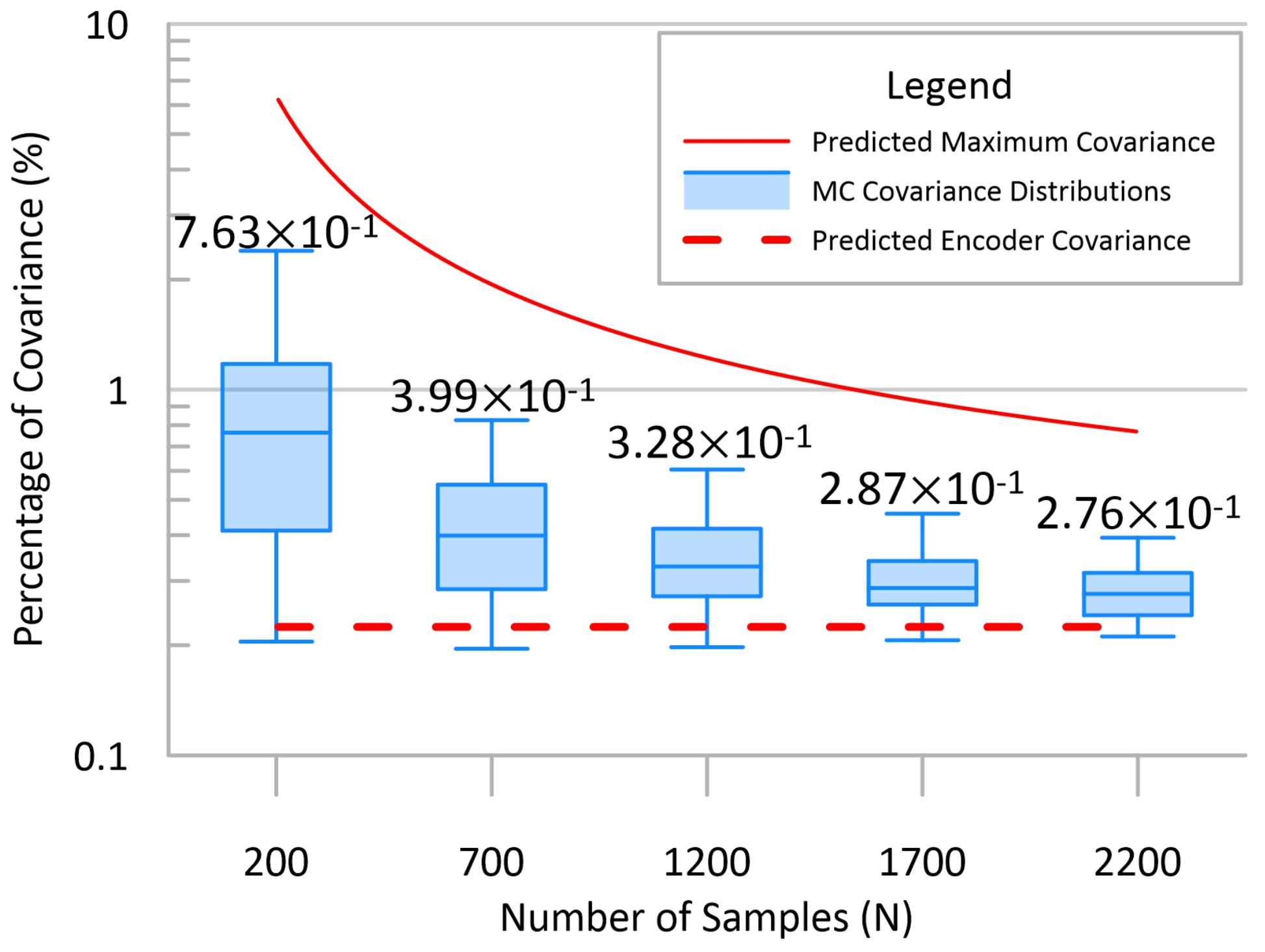
The relationships between expected pose uncertainty and data set size described in (41) and (44) are validated by performing Monte Carlo analysis on randomly selected subsets of the simulated data. Calibration and velocity Jacobians are generated for each selected pose along with a single random pose covariance matrix scaled such that its trace matches that of the arbitrary baseline case. The expected Jacobians in each trial are formed by taking the element-wise mean of the respective point-wise matrices. Trial-invariant covariance matrices representing uniformly distributed encoder uncertainty are included in each trial. The trial covariance traces are combined and converted to percentages of the covariance traces found in the minimum calibration case in which only twelve 6 DoF pose measurements are present. The percentage distributions for trials at specified data point intervals are compared to the baseline encoder uncertainty levels and expected covariance trace values in Figure 4.

The validation trials display overestimation of final pose covariance for the simulated manipulator. The large workspace volume covered by the simulated points results in a worst-case scenario, as the linear nature of the expected Jacobian cannot fully capture the highly non-linear behavior of the manipulator. As all trial values are bounded by the estimated pose covariance, conservative estimates for calibration data set sizes can be safely generated with (45).

3.3. Simulated Hybrid Manipulator Calibration

To more robustly test the calibration framework and ensure that convergence is observed over the entire workspace, repeated calibration trials are performed on copies of the perturbed model. A total of 100 trials are completed, with each trial using a 700 pose sub-set of the 20,000 simulated calibration poses. Jacobian dimensions in each trial are defined by (35) are [4200 × 68]. The number of poses chosen for each sub-set is informed by the breakpoint for diminishing returns of expected covariance as displayed in Figure 4. Each subset is selected randomly without replacement and is generated at the beginning of each trial. Measurement uncertainty is added to each data set during the trial; uncertain data sets are not shared between trials nor is uncertainty information permanently associated with any individual data point.

Each calibration trial typically reached exit conditions in 3 epochs. Standard Gauss–Newton steps described in (7) are taken with a pseudoinverse cutoff ratio of 1:500 used to permit calibration of less observable variables. An additional constraint and error pair corresponding to each calibrated unit quaternion is appended to the previously described calibration Jacobian to ensure that only steps that retain the unit quaternion format are taken.

Each of the calibrated parameterizations is validated with the previously generated set of 2000 validation poses not used within the calibration process. Each trial utilizes the same baseline validation data set, although measurement uncertainty is added independently in each. Pose-error values for each trial are generated for validation data set in cases with and without added measurement uncertainty. A scalar metric of performance is found by separately taking the root-mean-square (RMS) values of the position and rotation components for each generated error vector. The distributions of the RMS pose-error residuals before and after calibration for all trials are displayed in Figure 5.

It is important to note that the error terms generated from validation poses without measurement uncertainty fall below those with measurement uncertainty, indicating that for well modelled high precision mechanisms such as parallel manipulators, pose-error becomes bounded by measurement uncertainty during the fitting process. The calibration fitting process is capable of reducing kinematic pose-error below this measurement uncertainty threshold in cases with sufficiently large data sets. This can best be observed in simulated cases such as presented by merit of being able to generate perfect measurements.

3.4. Experimental Manipulator Description

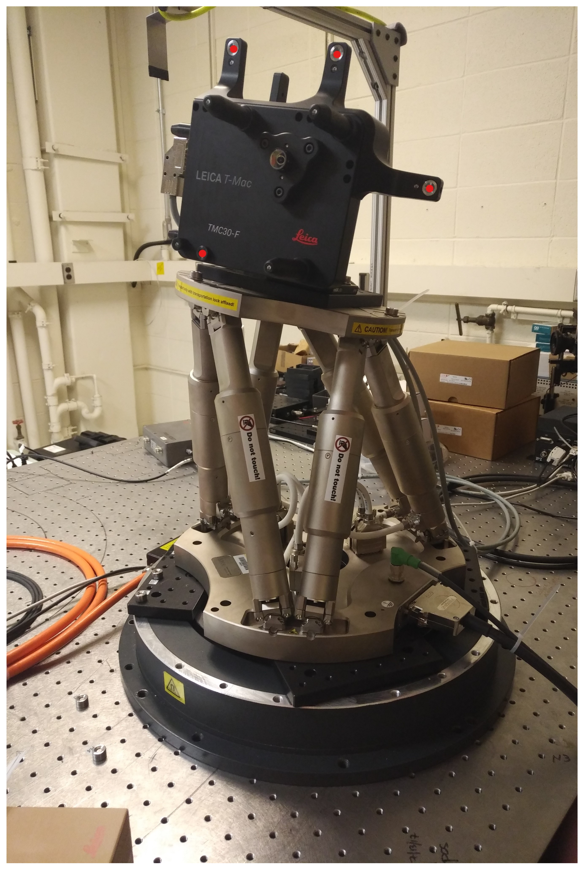
The developed calibration approach is used to characterize a physical hybrid manipulator. Compared to the high-complexity simulation used for validating the calibration approach, this test case demonstrates the procedure’s effectiveness with real measurement uncertainties introduced by the metrology system and a nominal parameterization based on a commercial parallel manipulator.

A simple hybrid manipulator was constructed using a commercially available 6-RRRPRR parallel manipulator with offset R-R joints (H-850 6-Axis Hexapod, Physik Instrumente, Karlsruhe, Germany. Commercial products or brand names are only mentioned to clarify what was done in this work. This is not an endorsement of any particular commercial product.) and rotary stage (ACR240HT-ABS, IntelLiDrives, Philadelphia, PA, USA. Commercial products or brand names are only mentioned to clarify what was done in this work. This is not an endorsement of any particular commercial product.). Both robot components are fully calibrated individually, and represent the state-of-the-art calibration baseline to which we compare our methods.

Pictured in Figure 6, the robots were securely mounted together and affixed to a precision optical table. To facilitate multiple data collection methods, laser tracker spherical targets (Red Ring Reflector 0.5${}^{″}$, Leica Geosystems, Norcross, GA, USA. Commercial products or brand names are only mentioned to clarify what was done in this work. This is not an endorsement of any particular commercial product.) were mounted in an asymmetric pattern to the top of parallel manipulator.

3.4.1. Encoder Information

Encoder information for each of the actuated joints within the experimental hybrid manipulator is listed in

Table 4. Actuated Joint Encoder and Variance Information.

Variable:	Encoder Resolution	Variance
Rotary Stage	2,097,152 counts/rot	7.4803 × 10${}^{-13}$ rad${}^2$
Prismatic Leg	40,960 counts/mm	4.9671 × 10${}^{-17}$ m${}^2$

with calculated variance terms. Each of the legs of the parallel manipulator has identical construction and share a single row. Encoder counts are multiplied by any intermediate gearing to yield final effective resolution. Variance is calculated based on a uniform distribution of width matching one encoder count in the pose-error units of meters and radians.

3.4.2. Identification of Coordinate Systems

Consistent world and end-effector frames are necessary for calibration. Although the laser tracker used for pose measurements within this work (Leica Absolute Tracker AT960, Leica Geosystems, Norcross, GA, USA. Commercial products or brand names are only mentioned to clarify what was done in this work. This is not an endorsement of any particular commercial product.) generates a measurement frame, the points can be recorded in reference to an arbitrarily positioned world frame. A coordinate frame with the z-axis nominally centered and normal to the rotary stage motion was defined using 3 DoF measurements recorded during motion. This world frame is referenced to static spherical target monuments (Leica Red-Ring Reflector 0.5${}^{″}$ (Commercial products or brand names are only mentioned to clarify what was done in this work. NIST does not endorse commercial products. Other products may work as well or better.)) attached to the table in Figure 6 and serves as the nominal proximal frame for the hybrid robot model. Frame errors compensated for by positioning the proximal frame with a calibrated offset.

The frame generated by a 6 DoF target at the home position served as the virtual end-effector for the hybrid manipulator and is used to determine the nominal distal offset. To allow for multiple measurement methods, this frame is also referenced to the spatial locations of the four spherical target nests integrated in the sensor.

3.4.3. Kinematic Model and Parameter Identification

The parallel manipulator kinematic model is implemented as described above, with parameterization listed in Appendix B. Offsets at the proximal and distal ends of the hybrid manipulator and between manipulator components are calibrated to compensate for the poorly defined initial states. Parameters for each of the manipulators were estimated with physical measurements and available CAD models.

Identifiable parameters within the kinematic model are determined by singular value analysis. Although singular values below a specified threshold of are removed during the pseudoinverse generation process, it is important to reduce the model to a minimal state for increased effectiveness of the calibration process and reduced computation time.

A concatenated calibration Jacobian is generated from an experimental data set described below. To ensure appropriate parameter steps, the column scaling is applied to the Jacobians such that a unitary parameter change would result in an RMS error change of 1 × 10${}^{-5}$[51]. By identifying the parameters listed as primary components in the $\mathbf{V}$ columns associated with the singular values with a condition number below 1:500, the parameter list is reduced significantly. Several parameters related to parallel member link lengths are retained despite falling below this value for model completeness and to test the impacts of different condition number cutoff points during calibration. It is noted by inspection that many of the poorly identifiable parameters removed overlap with either retained kinematic parameters or passive joint components within individual parallel members. The limited workspace of the experimental parallel manipulator results in the lack of rigorous exercise of all degrees of freedom on parallel members leading to poor identifiability. The permitted condition number is expanded to 1:1000 in the calibration experiments in the interest of capturing some of these poorly identifiable degrees of freedom in the hybrid manipulator throughout the experiments below. A total of 53 kinematic parameters were calibrated, of which 48 were incorporated in the parallel manipulator and evenly distributed to the constituent parallel members. A listing of the calibrated parameters within this case study is found in

Table A4. Experimental hybrid manipulator parameters.

Link	Type	Variable
		$\mathit{a}$	$\mathit{\alpha }$	$\mathit{\beta }$	$\mathit{d}$	$\mathit{\theta }$	$\mathit{\gamma }$	$\mathit{p}$
Proximal Offset	PQ							[1,1,0]
Rotary Stage	HR	1	0	0		A	0
Int. Offset	PQ							[0,0,1]
Parallel Member	PQ							[1,1,0]
	DHR	1	0		0	P	0
	DHR	0	0		0	P	0
	HP	0	0	0	A	0	1
	DHR	0	0		0	P
	DHR	1	0		0	P
	DHR	0	1		0	P
	PQ							[1,1,0]
Distal Offset	PQ							[0,0,1]

.

3.5. Experimental Pose Data Collection

To allow for accurate measurement of the pose of the robotic manipulator, sets of four laser tracker spherical targets are mounted asymmetrically to the end-effector as shown in Figure 6. Each target is measured in 3 DoF by the laser tracker system previously detailed and a 6 DoF end-effector pose is generated by fitting each point cloud to a nominal relationship of the mounting points to a virtual frame definition. A total of 200 randomized poses are generated for the hybrid manipulator within the supported motion ranges such that all of the spherical targets remain in view of the laser tracker system. The hybrid manipulator home position is recorded in this manner and included in the data set. The motion of the rotary stage is constrained to $\pm \frac{\pi }{4}$ radians to prevent cable breakage.

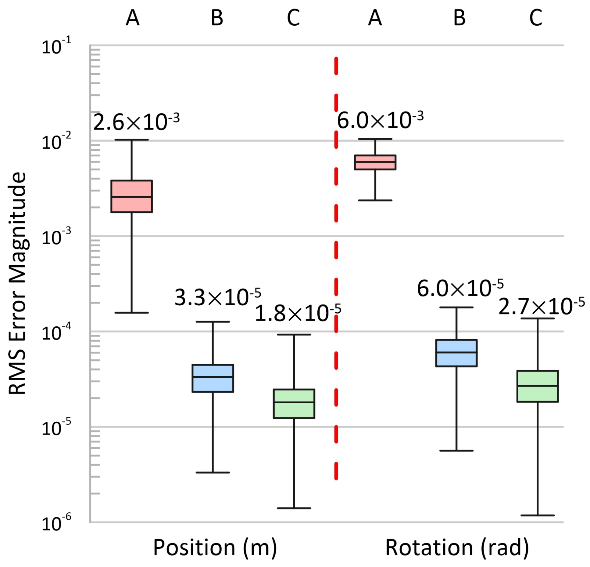
Laser tracker measurement uncertainty is dependent on the distance between the spherical target and the measurement head with manufacturer specification $\pm 7.5\mathsf{\mu }$m + $3\mathsf{\mu }$m/m for 3 DoF points [52]. A 3 × 3 covariance matrix $\Sigma$ is returned by the data collection software for each point measurement, which is converted to mean standard deviation using (40). The resultant distribution of uncertainty values calculated in this manner is displayed in Figure 7, with low variation observed due to the small workspace of the experimental manipulator.

Encoder values for controllable joint parameters are converted into appropriate input variables $\theta$, with rotary stage position reported with units of radians and parallel manipulator leg-lengths reported with units of millimeters.

Frame Reconstruction and Uncertainty

Pose reconstruction is implemented as SVD-based point cloud fitting [53], which calculates the transform between two ordered sets of 3D points while minimizing the least squares error. Provided a known home position in the world frame, the transform between a point groups collected at the hybrid manipulator home position and a calibration pose is used to determine the final pose.

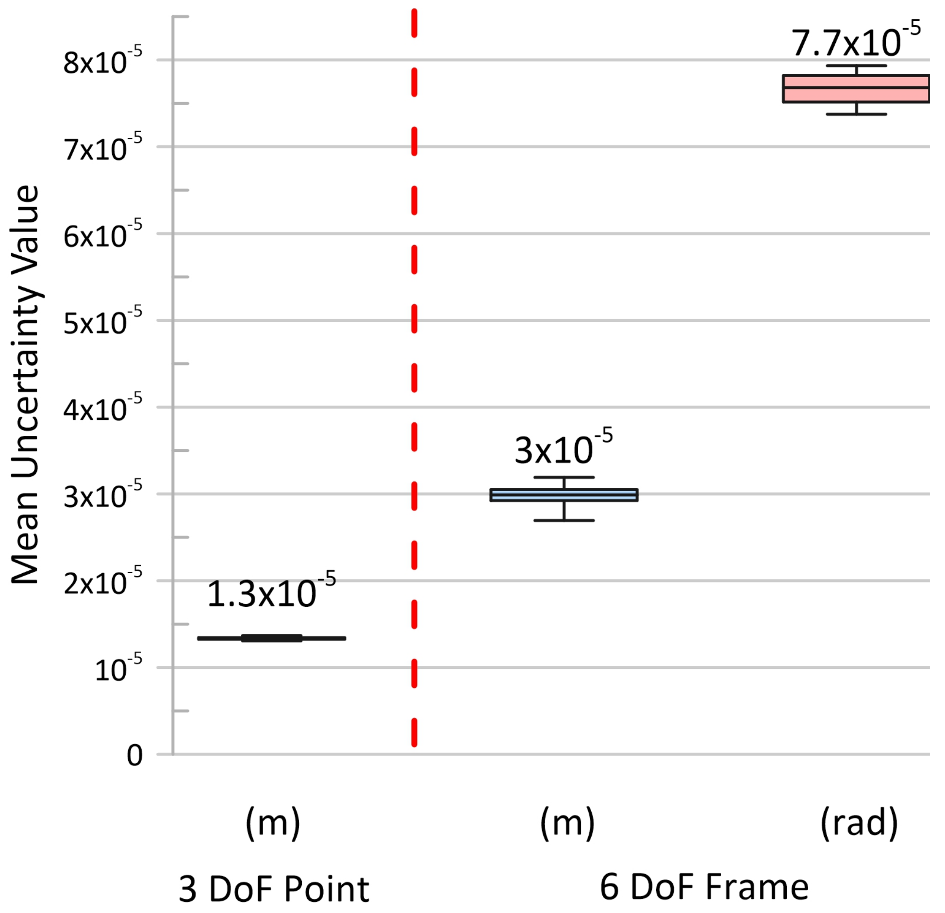
Sets of 3D point measurements acquired by a laser tracker can be used to construct 6 DoF pose measurements. The calculation of pose uncertainties of a 6 DoF pose derived from a set of N point (3D) measurements is detailed below.

For a series of N point measurements, the final covariance matrix for a single pose is represented as

$${\Sigma }_m=\left[\begin{array}{cccc}{\Sigma }_1& \mathbf{0}& \cdots & \mathbf{0}\\ \mathbf{0}& {\Sigma }_2& \cdots & \mathbf{0}\\ ⋮& ⋮& \ddots & ⋮\\ \mathbf{0}& \mathbf{0}& \cdots & {\Sigma }_N\end{array}\right],$$

(46)

where $\Sigma$ is a 3 × 3 covariance matrix for a point indicated by the subscript.

The relationship between the combined covariances and pose-error as defined in (4) is facilitated by representing the transform of a manipulator in the $\mathbf{p}\&\mathbf{q}$ format detailed in Appendix A. The calibration Jacobian defined for this construct can be utilized to model the uncertainties of the least squares fitting process as

$${\mathbf{J}}_{\mathrm{p}}=\frac{\partial \mathbf{e}}{\partial \mathbf{\tau }}{\left(\frac{\partial \mathbf{p}}{\partial {\mathbf{\tau }}^{\prime }}\right)}^{†}$$

(47)

where $\frac{\partial \mathbf{e}}{\partial \mathbf{\tau }}$ is the [6 × 7] analytical Jacobian for a $\mathbf{p}\&\mathbf{q}$ offset link representing the optimal transform as specified in Appendix A. Individual point measurements relative to the frame are added to the $\mathbf{p}\&\mathbf{q}$ offset separately, with the resulting combinations used to generate an analytical Jacobian at each point. The Jacobian rows related to the position error terms are vertically concatenated to form $\frac{\partial \mathbf{p}}{\partial {\mathbf{\tau }}^{\prime }}$, a [3$N\times$ 7] matrix where N is the number of 3D point measurements included in point group $\mathbf{p}$.

The combined Jacobian ${\mathbf{J}}_{\mathrm{p}}$ are used to propagate the measurement covariance using form (38) as

$${\Sigma }_p={\mathbf{J}}_p{\Sigma }_m{\mathbf{J}}_p^{\top },$$

(48)

where ${\Sigma }_p$ is a 6 × 6 matrix which represents the final measurement uncertainties and couplings present in each 6 DoF pose. The order of the terms corresponds to that found within the standard pose-error vector within this work (4). The uncertainty distributions for the reconstructed frames used in this calibration are displayed in Figure 7. For the reconstructed frames, the uncertainties associated with the rotation parameters are significantly higher than those related to position terms.

3.6. Experimental Hybrid Manipulator Calibration

Calibration of the as-assembled hybrid manipulator was conducted in a two step process. First, errors introduced during assembly are compensated for by calibrating pose offsets introduced between the manipulator components and at the distal and proximal ends of the manipulator. The nominal parameters of the rotary stage and parallel manipulator are not calibrated in this case to preserve the baseline accuracy of the components. Using the full data set inclusive of manipulator home position, this calibration process yields 118 $\mathsf{\mu }$m RMS position error and 182 $\mathsf{\mu }$rad RMS rotation error. This offset compensation case is considered representative of the hybrid manipulator accuracy without the calibration techniques developed in this work.

The second step expands the scope of the calibration to include kinematic parameters of the rotary stage and parallel manipulator components in addition to the pose offsets identified in the prior step. Calibration was conducted using a random selection with no replacement of 70% of the data set collected inclusive of the manipulator home position and rounded up. For the subset of 141 poses, calibration Jacobian dimensions as defined by (35) are [846 × 53]. The calibration terminated after three epochs upon reaching the parameter change exit condition, with 91.1 $\mathsf{\mu }$m RMS position error and 64.1 $\mathsf{\mu }$rad rotation error using a singular value cutoff ratio of 1:1000. The updated parameterization was validated with the remaining 30% of the poses from the original data set that were not used within the calibration process, resulting in 90.4 $\mathsf{\mu }$m RMS position error and 76.8 $\mathsf{\mu }$rad rotation error. The calibration process was repeated with the complete 201 point data set, achieving a final 91.1 $\mathsf{\mu }$m RMS position error and 71.2 $\mathsf{\mu }$rad rotation error. This represents a 46.7% reduction in error compared to the baseline assembly offset calibration case.

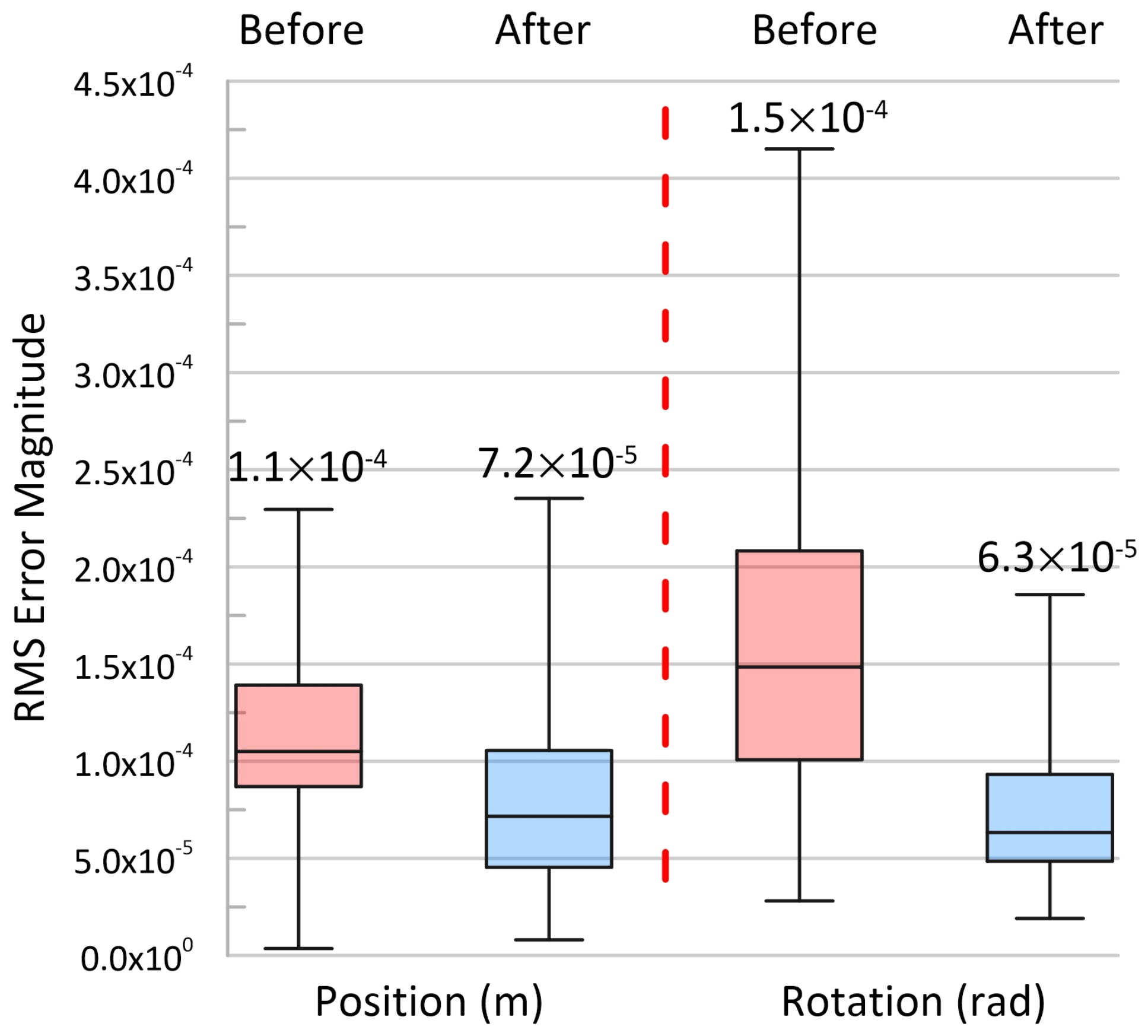
Pose-error distributions for the validation data set are generated for the calibrated and uncalibrated hybrid manipulator and converted into scalar distributions by separately taking the RMS of the position and rotation components of the error vector at each pose. The resultant distributions are displayed in Figure 8 and exist near the identified measurement uncertainties for the laser tracker system. Measurement uncertainty cannot be stripped from the measurements outside of simulation, but it is anticipated that the real performance of the calibration falls below the measurement uncertainty of the laser tracker.

3.7. Comparison to Alternate Calibration Methods

Kinematic loop closure calibration methods are implemented on the parallel manipulator portion of the hybrid manipulator. These established methods have been adapted to the parallel manipulator geometry of interest as demonstrated in [54], but have been widely implemented for use on canonical Stewart Platform manipulator designs [23] and other novel parallel mechanisms [20]. Each implementation minimizes a scalar representation of the position error found within specified kinematic chains, referred to as Position Vector Loop Closure (PVLC) in this work. Within this work, a basic implementation in which the position error between the end effector of each parallel leg $m\in \mathbf{M}$ and the manipulator transform ${\mathbf{T}}_{\mathrm{parallel}}$ at each measurement is minimized with serial Jacobians generated using the passive joint parameters $\mathbf{\psi }$ found by solving the inverse kinematics to reach the measured ${\mathbf{T}}_{\mathrm{parallel}}$ and actual leg length measurements $\mathbf{\varphi }$. This configuration is chosen to most closely match contemporary literature. After the loop closure calibration has been completed, the serial manipulator offset calibration is repeated to ensure convergence.

The Nelder–Mead simplex method has been implemented in contemporary literature for final optimization of a novel 6 DoF parallel manipulator after coarse calibration has been completed [33]. This approach is implemented using the MATLAB general minimization function fminsearch, with evaluation function corresponding to the RMS of the total pose-error vector $\mathbf{E}$. As no options are specified in the corresponding work, default termination options are retained.

Contemporary literature has implemented Hybrid Genetic Algorithm (HGA) fitting on a variety of parallel manipulators with comparisons to alternate calibration approaches [29]. This approach is composed of genetic algorithm minimization followed by gradient-based constrained minimization facilitated by the MATLAB optimization functions ga and fmincon, respectively. The option settings are adjusted to a crossover fraction of 0.7, a population size of 100 with 3000 maximum generations. Function tolerance is specified to 1 × 10${}^{-100}$, with hybrid function specified to use SQP. As the use of genetic algorithm methods greatly impacts computational performance, a trial calibration is also performed with only the gradient-based fmincon function for comparison purposes. Options are identical to the prior case. Parallel computation is enabled to improve optimization performance for both related test cases.

The final pose-error found by each of the described calibration approaches and associated computation time are listed and compared to both the baseline hybrid manipulator parameterization and our approach (Constrained NLS) in

Table 5. Alternate Calibration Method Comparison.

Calibration Type	RMS Pos. Error ($\mathsf{\mu }$m)	RMS Rot. Error ($\mathsf{\mu }$rad)	Runtime ${}^{*}$ (s)
Constrained NLS	91.1	71.2	14.9
Serial NLS ${}^{†}$ [30]	118	182	10.8
PVLC ${}^{‡}$ [20,21,27]	133	168	104
Nelder–Mead [33]	118	182	5150
HGA [29]	118	182	6280
fmincon [29]	118	182	161

${}^{*}$ Single run timing on MATLAB 2018b with Intel-i7-4700MQ CPU@2.40GHz and 32 GB Memory, ${}^{†}$ Calibration of assembly offsets using serial manipulator techniques to reach baseline parameter set, ${}^{‡}$ Best result with early termination.

. In the Nelder–Mead, HGA, and fmincon cases, the pose-error of the manipulator was not reduced from the baseline parameterization. Results for these comparisons are discussed in the following section.

4. Discussion

4.1. Alternate Calibration Methods

To compare our calibration approach to the methods outlined above, it is important to note operational behavior of each type. As [20] and later [10] noted, the closed loop calibration method without passive joint measurements can fail to converge for some parameter sets. Similar behavior was found in the experimental calibration of the hybrid manipulator, with pose-error of the manipulator increasing as the position-based loop residuals were reduced. This behavior matches the prior observations that such methods were very sensitive to measurement noise. Simple cases in which the measured end-effector position of the parallel manipulator are used to perform loop closure on individual kinematic chains cannot generally be applied unless parameter sets are carefully selected and tested and typically only minimize position components of the total pose-error of interest. Slow convergence is noted due to the updates to the estimated passive joint parameters and lack of consideration for such changes in each kinematic parameter update step.

Non-gradient optimization methods based on the Nelder–Mead simplex algorithm have been implemented within the MATLAB environment over the selected parameter set with an evaluation function corresponding to the RMS of the total pose-error residuals. The evaluation function was not improved on a relevant scale during calibration, with 1.1709 × 10${}^{-17}$ of calculated RMS reduction, and exited after 438 iterations after convergence. Two factors hamper the effectiveness of this direct-search method: the large dimensionality of the calibrated kinematic parameters, which greatly slows the performance of the search, and the presence of a local minima at the initial minimization conditions created by the baseline calibration pass. Although simplified kinematic parameter sets can be used to improve the performance of this method, the high dimensionality and very nonlinear behavior of parallel manipulators makes this approach unsuitable for general use.

The hybrid genetic algorithm fitting method is a general optimization method employed over the selected parameter set with the evaluation function to be minimized corresponding to the RMS of the total pose-error residuals. When implemented with the options detailed in [29], the genetic algorithm component did not reduce pose-error from the baseline case, and the subsequent fmincon constrained optimization routine exited after one iteration due to minimum step tolerances below the specified 1 × 10${}^{-7}$. Once again, the local minima of the starting conditions generated by the baseline serial pose-error calibration case are difficult to escape. Parallelization helps offset the cost of the genetic algorithm component, but computation time is longer than any other minimization method due to its inclusion.

A direct call to fmincon yields identical results significantly faster. This method uses minimization methods on a gradient numerically calculated for the evaluation function. This gradient-based approach suffers from compressing the pose-error dimensions and the direct computation approach, in which parameter steps are used to approximate the gradient. As seen in the Serial NLS calibration case, parameter updates can increase position error while reducing rotation error. When evaluating the total pose-error vector as a scalar quantity, this information is lost. The direct computation of this gradient on a highly nonlinear system compounds the problem, resulting in early termination due to step sizes falling below the specified threshold of 1 × 10${}^{-7}$.

4.2. Application Overview

The calibration and kinematic framework presented is modular and can be applied to any robot manipulator construction. Extensive testing on cases with multiple parallel manipulators or nested parallel constructions are outside of the scope of the intended application of this work and are omitted from consideration during validation process. Case-by-case evaluation must be conducted to determine an efficient implementation for these algorithms.

4.3. Uncertainty Conclusions

The calibration process in both simulated and experimental cases yielded calibrated pose uncertainty near that of the measurement system when validation poses with measurement uncertainty were used. In the case of the simulated data without measurement uncertainty, it is noted that the pose-error falls significantly below this mark, indicating that the calibration procedure is capable of reducing error below the measurable threshold. As all real measurements contain uncertainty, this motivates the modelling of post-calibration uncertainty to inform pose selection and data set size to reach desired uncertainty levels below measurable levels. Although this process cannot impact the pose uncertainty caused by discrete encoder counts, it minimizes the uncertainty added by physical phenomenon such as gravitational loading and bending effects that are captured in pose measurements. Pose-error introduced by these phenomenon are captured during data collection and minimized by the kinematic parameter calibration, resulting in parameters that best capture the kinematic performance of the manipulator but may not directly correspond to physical dimensions.

In the experimental test case, the calibrated uncertainty remains above the measurement uncertainty values. The limited workspace of the experimental hybrid manipulator does not permit all joints to be extensively exercised, resulting in low identifiability of the parameters during the calibration process. Joint motion is further limited by the data collection process as all spherical targets must maintain line-of-sight with the measurement system. Alternate configurations that permit additional joint motion during measurement, such as altering spherical target placement or incorporating measurements from a secondary laser tracker unit, will increase parameter identifiability and reduce final calibrated uncertainty.

4.4. Future Work

The pose covariance model discussed in this work as a method of determining post-calibration pose uncertainty can be extended to include all possible poses through simultaneous fitting of the measurement uncertainty model. Given a series of pose measurements with pose uncertainty, a cyclic fitting process such as expectation-maximization can be applied to a parameterized representation of the measurement system during the calibration process [55]. The resultant model can be used to characterize measurement uncertainty—and therefore calibrated pose uncertainty - over the entire workspace. This can be used to determine more accurate bounds for estimated calibration data set sizes or pose selection and path planning that minimizes known uncertainty.

5. Conclusions

A unified and computationally efficient calibration framework based on null space constraint propagation was developed that extends established serial manipulator techniques to parallel and hybrid manipulators composed of both parallel and serial manipulators. Kinematic models based on this approach were presented and validated on both simulated and experimental hybrid manipulators. Notably, a reduction to 91.1 $\mathsf{\mu }$m RMS position error and 71.2 $\mathsf{\mu }$rad RMS rotation error was observed using the methods outlined in this work. A generalized uncertainty estimation framework was also developed that can accurately characterize the residual uncertainty found at calibrated poses or those measured with known uncertainty. This model was used to guide the calibration data set size selection to meet desired uncertainty levels in the case studies.

References

1. Campos, L.; Bourbonnais, F.; Bonev, I.A.; Bigras, P. Development of a Five-Bar Parallel Robot With Large Workspace. In Proceedings of the 34th Annual Mechanisms and Robotics Conference, Parts A and B. ASMEDC, Montreal, QC, Canada, 15–18 August 2010; Volume 2. [Google Scholar] [CrossRef] [Green Version]
2. Danko, T.W.; Chaney, K.P.; Oh, P.Y. A parallel manipulator for mobile manipulating UAVs. In Proceedings of the IEEE International Conference on Technologies for Practical Robot Applications (TePRA), Woburn, MA, USA, 11–12 May 2015; IEEE: Piscataway, NJ, USA, 2015. [Google Scholar] [CrossRef]
3. Han, H.; Han, C.Y.; Xu, Z.B.; Zhu, M.C.; Yu, Y.; Wu, Q.W. Kinematics analysis and testing of novel 6-P-RR-R-RR parallel platform with offset RR-joints. Proc. Inst. Mech. Eng. C J. Mech. Eng. Sci. 2018, 233, 3512–3530. [Google Scholar] [CrossRef]
4. Tanev, T.K. Kinematics of a hybrid (parallel–serial) robot manipulator. Mech. Mach. Theory 2000, 35, 1183–1196. [Google Scholar] [CrossRef]
5. Gordon, J.A.; Novotny, D.R.; Francis, M.H.; Wittmann, R.C.; Butler, M.L.; Curtin, A.E.; Guerrieri, J.R. Millimeter-Wave Near-Field Measurements Using Coordinated Robotics. IEEE Trans. Antennas Propag. 2015, 63, 5351–5362. [Google Scholar] [CrossRef]
6. Kucuk, S.; Gungor, B.D. Inverse kinematics solution of a new hybrid robot manipulator proposed for medical purposes. In Proceedings of the 2016 Medical Technologies National Congress (TIPTEKNO), Antalya, Turkey, 27–29 October 2016; IEEE: Piscataway, NJ, USA, 2016. [Google Scholar] [CrossRef]
7. Stewart, D. A Platform with Six Degrees of Freedom. Proc. Inst. Mech. Eng. 1965, 180, 371–386. [Google Scholar] [CrossRef]
8. Gough, V.E. Universal tyre test machine. In Proceedings of the FISITA 9th International International Automobile Technical Congress, London, UK, 30 April–5 May 1962. [Google Scholar]
9. Gloess, R.; Lula, B. Challenges of extreme load hexapod design and modularization for large ground-based telescopes. Modern Technologies in Space-and Ground-based Telescopes and Instrumentation. In Proceedings of the SPIE, San Diego, CA, USA, 27 June–2 July 2010. [Google Scholar] [CrossRef]
10. Wampler, C.W. Forward displacement analysis of general six-in-parallel sps (Stewart) platform manipulators using soma coordinates. Mech. Mach. Theory 1996, 31, 331–337. [Google Scholar] [CrossRef]
11. Cheok, K.C.; Overholt, J.L.; Beck, R.R. Exact methods for determining the kinematics of a stewart platform using additional displacement sensors. J. Robotic Syst. 1992, 10, 689–707. [Google Scholar] [CrossRef]
12. Liu, K.; Fitzgerald, J.M.; Lewis, F.L. Kinematic analysis of a Stewart platform manipulator. IEEE Trans. Ind. Electron. 1993, 40, 282–293. [Google Scholar] [CrossRef]
13. Merlet, J. Direct kinematics of parallel manipulators. IEEE Trans. Robot. Autom. 1993, 9, 842–846. [Google Scholar] [CrossRef]
14. McAree, P.R.; Daniel, R.W. A Fast, Robust Solution to the Stewart Platform Forward Kinematics. J. Robot. Syst. 1996, 13, 407–427. [Google Scholar] [CrossRef]
15. Everett, L.J. Forward Calibration of Closed-Loop Jointed Manipulators. Int. J. Robot. Res. 1989, 8, 85–91. [Google Scholar] [CrossRef]
16. Staicu, S. Dynamics of the 6-6 Stewart parallel manipulator. Robot. Comput.-Integr. Manuf. 2011, 27, 212–220. [Google Scholar] [CrossRef]
17. Chaudhury, A.N.; Ghosal, A. Optimum design of multi-degree-of-freedom closed-loop mechanisms and parallel manipulators for a prescribed workspace using Monte Carlo method. Mech. Mach. Theory 2017, 118, 115–138. [Google Scholar] [CrossRef]
18. Zhuang, H.; Roth, Z.S. Method for kinematic calibration of stewart platforms. J. Robot. Syst. 1993, 10, 391–405. [Google Scholar] [CrossRef]
19. Khalil, W.; Besnard, S. Self calibration of Stewart-Gough parallel robots without extra sensors. IEEE Trans. Robot. Autom. 1999, 15, 1116–1121. [Google Scholar] [CrossRef] [Green Version]
20. Hollerbach, J.; Lokhorst, D. Closed-loop kinematic calibration of the RSI 6-DOF hand controller. IEEE Trans. Robot. Autom. 1995, 11, 352–359. [Google Scholar] [CrossRef]
21. Wampler, C.W.; Hollerbach, J.; Arai, T. An implicit loop method for kinematic calibration and its application to closed-chain mechanisms. IEEE Trans. Robot. Autom. 1995, 11, 710–724. [Google Scholar] [CrossRef]
22. Zhuang, H.; Liu, L. Self-calibration of a class of parallel manipulators. In Proceedings of the IEEE International Conference on Robotics and Automation, Minneapolis, MN, USA, 22–28 April 1996; IEEE: Piscataway, NJ, USA, 1996. [Google Scholar] [CrossRef]
23. Zhuang, H.; Yan, J.; Masory, O. Calibration of stewart platforms and other parallel manipulators by minimizing inverse kinematic residuals. J. Robot. Syst. 1998, 15, 395–405. [Google Scholar] [CrossRef]
24. Masory, O.; Wang, J.; Zhuang, H. On the accuracy of a Stewart platform. II. Kinematic calibration and compensation. In Proceedings of the IEEE International Conference on Robotics and Automation, Atlanta, GA, USA, 2–6 May 1993; Volume 1, pp. 725–731. [Google Scholar] [CrossRef]
25. Chai, K.S.; Young, K.; Tuersley, I. A practical calibration process using partial information for a commercial Stewart platform. Robotica 2002, 20, 315–322. [Google Scholar] [CrossRef]
26. Meng, G.; Tiemin, L.; Wensheng, Y. Calibration method and experiment of Stewart platform using a laser tracker. In Proceedings of the IEEE International Conference on Systems, Man and Cybernetics, Washington, DC, USA, 8 October 2003; Volume 3, pp. 2797–2802. [Google Scholar] [CrossRef]
27. Han, C.; Yu, Y.; Xu, Z.; Wang, X.; Yu, P.; Zhou, X. Complete kinematic calibration of a 6-RRRPRR parallel kinematic machine based on the optimal measurement configurations. Proc. Inst. Mech. Eng. C J. Mech. Eng. Sci. 2019, 234, 121–136. [Google Scholar] [CrossRef]
28. Okamura, K.; Park, F. Kinematic calibration using the product of exponentials formula. Robotica 1996, 14, 415–421. [Google Scholar] [CrossRef]
29. Sun, T.; Lian, B.; Yang, S.; Song, Y. Kinematic Calibration of Serial and Parallel Robots Based on Finite and Instantaneous Screw Theory. IEEE Trans. Robot. 2020, 36, 816–834. [Google Scholar] [CrossRef]
30. Bennett, D.J.; Hollerbach, J.M. Autonomous calibration of single-loop closed kinematic chains formed by manipulators with passive endpoint constraints. IEEE Trans. Robot. Autom. 1991, 7, 597–606. [Google Scholar] [CrossRef]
31. Mayer, R.; Oliviers, M.P. Global kinematic calibration of a Stewart platform. In Proceedings of the ASME Dynamic Systems and Control Division, San Francisco, CA, USA, 12–17 November 1995; Volume 57. [Google Scholar]
32. Ibaraki, S.; Yokawa, T.; Kakino, Y.; Nakagawa, M.; Matsushita, T. Kinematic calibration on a parallel kinematic machine tool of the Stewart platform by circular tests. In Proceedings of the 2004 American Control Conference, Boston, MA, USA, 30 June–2 July 2004; IEEE: Piscataway, NJ, USA, 2004. [Google Scholar] [CrossRef]
33. Wu, J.F.; Zhang, R.; Wang, R.H.; Yao, Y.X. A systematic optimization approach for the calibration of parallel kinematics machine tools by a laser tracker. Int. J. Mach. Tools Manuf. 2014, 86, 1–11. [Google Scholar] [CrossRef]
34. Sun, T.; Zhai, Y.; Song, Y.; Zhang, J. Kinematic calibration of a 3-DoF rotational parallel manipulator using laser tracker. Robot. Comp.-Integr. Man. 2016, 41, 78–91. [Google Scholar] [CrossRef]
35. Song, Y.; Zhang, J.; Lian, B.; Sun, T. Kinematic calibration of a 5-DoF parallel kinematic machine. Precis. Eng. 2016, 45, 242–261. [Google Scholar] [CrossRef]
36. Huang, P.; Wang, J.; Wang, L.; Yao, R. Kinematical calibration of a hybrid machine tool with Regularization method. Int. J. Mach. Tools Manuf. 2011, 51, 210–220. [Google Scholar] [CrossRef]
37. Liu, Y.; Wu, J.; Wang, L.; Wang, J. Parameter identification algorithm of kinematic calibration in parallel manipulators. Adv. Mech. Eng. 2016, 8. [Google Scholar] [CrossRef] [Green Version]
38. Chen, G.; Kong, L.; Li, Q.; Wang, H.; Lin, Z. Complete, minimal and continuous error models for the kinematic calibration of parallel manipulators based on POE formula. Mech. Mach. Theory 2018, 121, 844–856. [Google Scholar] [CrossRef]
39. Jokiel, B.; Ziegert, J.C.; Bieg, L. Uncertainty propagation in calibration of parallel kinematic machines. Precis. Eng. 2001, 25, 48–55. [Google Scholar] [CrossRef] [Green Version]
40. Murray, R.M.; Li, Z.; Sastry, S.S. A Mathematical Introduction to Robotic Manipulation; CRC Press: Boca Raton, FL, USA, 1994. [Google Scholar] [CrossRef] [Green Version]
41. Magnus, J. Matrix Differential Calculus with Applications in Statistics and Econometrics; John Wiley & Sons, Inc.: Hoboken, NJ, USA, 2019. [Google Scholar]
42. Hollerbach, J.; Khalil, W.; Gautier, M. Springer Handbook of Robotics; Chapter Model Identification; Springer: Berlin/Heidelberg, Germany, 2008; pp. 321–344. [Google Scholar]
43. Levenberg, K. A method for the solution of certain non-linear problems in least squares. Q. Appl. Math. 1944, 2, 164–168. [Google Scholar] [CrossRef] [Green Version]
44. Bonnans, J.F.; Gilbert, J.C.; Lemarechal, C.; Sagastizábal, C.A. Numerical Optimization: Theoretical and Practical Aspects; Springer: Berlin/Heidelberg, Germany, 2006. [Google Scholar]
45. Raghavan, M. The Stewart Platform of General Geometry Has 40 Configurations. J. Mech. Des. 1993, 115, 277–282. [Google Scholar] [CrossRef]
46. Hoffman, K.; Kunze, R. Linear Algebra, 2nd ed.; Prentice-Hall: Englewood Cliffs, NJ, USA, 1971. [Google Scholar]
47. Siciliano, B.; Sciavicco, L.; Villani, L.; Oriolo, G. Robotics: Modelling, Planning and Control; Springer: London, UK, 2010. [Google Scholar]
48. Taylor, B.N.; Kuyatt, C.E. Guidelines for Evaluating and Expressing the Uncertainty of NIST Measurement Results; NIST Technical Note 1297; NIST: Gaithersburg, MA, USA, 1994. [Google Scholar]
49. Wang, J.; Masory, O. On the accuracy of a Stewart platform. I. The effect of manufacturing tolerances. In Proceedings of the IEEE International Conference on Robotics and Automation, Atlanta, GA, USA, 2–6 May 1993. [Google Scholar] [CrossRef]
50. Wishart, J. The generalised product moment distribution in samples from a normal multivariate population. Biometrika 1928, 20A, 32–52. [Google Scholar] [CrossRef] [Green Version]
51. Schröer, K. Chapter Theory of kinematic modelling and numerical procedures for robot calibration. In Robot Calibration; Chapman & Hall: Boca Raton, FL, USA, 1993; pp. 157–196. [Google Scholar]
52. Hexagon Manufacturing. Leica Absolute Tracker AT960 Data Sheet; Cedar House: Minehead, UK, 2016. [Google Scholar]
53. Arun, K.; Huang, T.; Blostein, S. Least-squares fitting of two 3-D point sets. IEEE T Pattern Anal. IEEE Trans. Pattern Anal. Mach. Intell. 1987, PAMI-9, 698–700. [Google Scholar] [CrossRef] [PubMed] [Green Version]
54. Huang, T.; Zhao, D.; Yin, F.; Tian, W.; Chetwynd, D.G. Kinematic calibration of a 6-DOF hybrid robot by considering multicollinearity in the identification Jacobian. Mech. Mach. Theory 2019, 131, 371–384. [Google Scholar] [CrossRef]
55. Dempster, A.P.; Laird, N.M.; Rubin, D.B. Maximum likelihood from incomplete data via the EM algorithm. J. R. Statist. Soc. B 1977, 39, 1–22. [Google Scholar]
56. Shuster, M.; Junkins, J.; American Astronautical Society. A Survey of Attitude Representations; Journal of the Astronautical Sciences; American Astronautical Society: Springfield, VA, USA, 1993. [Google Scholar]
57. Hartenberg, R.S.; Denavit, J. A kinematic notation for lower pair mechanisms based on matrices. J. Appl. Mech. 1955, 77, 215–221. [Google Scholar]
58. Hayati, S.; Tso, K.; Roston, G. Robot geometry calibration. In Proceedings of the IEEE International Conference on Robotics and Automation, Philadelphia, PA, USA, 24–29 April 1988; Volume 2, pp. 947–951. [Google Scholar] [CrossRef]
Figure 1. CAD representation of a complex hybrid manipulator similar to that simulated for calibration approach validation. Hybrid manipulators can be used to extend the fine end-effector positioning of parallel manipulators over a large workspace.
Robotics 10 00124 g001
Figure 2. Robotic manipulators representative of those described in this work. Displayed as (A) parallel manipulator, (B) serial manipulator, and (C) hybrid manipulator.
Robotics 10 00124 g002
Figure 3. Notation representing the hybrid manipulator. Standard serial links are represented in green, with parallel members M 1 and M 2 formed from serial links in blue. Adjustable pose offsets are represented by dashed lines, while serial links are solid. Strictly serial links L 1 and L 2 share parameters across each serial chain. The length of links M 1 , 2 and M 2 , 2 and the joint angles of links L 1 and L 2 are actuated (active joints, θ ). All rotation joints within parallel members M 1 and M 2 are unactuated (passive joints, ψ ).
Robotics 10 00124 g003
Figure 4. Evolution of the trace of expected pose-error covariance with respect to data set size. Values are displayed as a percentage of the expected pose-error covariance found at the minimum necessary calibration data set of twelve 6 DoF poses for the hybrid manipulator. Median values are listed above each distribution. 100 trials were conducted for each N value to generate the actual distributions (blue). Distributions predicted by (44) are pictured in red, and show convergence with actual results as N .
Robotics 10 00124 g004
Figure 5. Validation data set error distributions for simulated hybrid manipulator calibration. Measurement uncertainty is added to each data point as described in Section 3.2. Initial error distributions (red, A) are significantly higher than calibrated error distributions (blue, B). Error distributions on the same validation data set without measurement uncertainty (green, C) indicate that the calibration procedure reduces error below the measurable uncertainty threshold. Median values are listed above each distribution, and a log axis scale is used to present the different magnitudes of data presented.
Robotics 10 00124 g005
Figure 6. Experimental 7 DoF hybrid robotic manipulator constructed from a 6-RRRPRR parallel manipulator with offset R-R joints mounted on a precision rotary stage. Spherical laser tracker target positions are marked with red. Laser tracker is not in view and is positioned approximately 2 meters from the manipulator without visual obstructions.
Robotics 10 00124 g006
Figure 7. Mean uncertainty distributions for the collected data set of 800 point measurements (3 DoF) and the resultant 200 reconstructed frames (6 DoF) used in the experimental calibration of Section 3.6. Mean uncertainties are defined as the square root of the trace of a covariance matrix divided by its degrees of freedom (40). In the case of the 6 DoF frame reconstruction, the position terms and rotation terms are considered separately to illustrate the relative magnitude of the components. Median values are listed above each distribution.
Robotics 10 00124 g007
Figure 8. Experimental error distributions for validation data set of 60 poses. Significantly larger pose-error distributions exist for the parallel manipulator in both position and rotation using manufacturer calibration (red) when compared to equivalent calibrated quantities (blue). Median values are listed above each distribution.
Robotics 10 00124 g008