Article

A Collision Avoidance Method Based on Deep Reinforcement Learning

1
Robotics and Mechatronics Lab, Department of Mechanical Engineering, Virginia Polytechnic Institute and State University, Blacksburg, VA 24061, USA
2
Torc Robotics, Blacksburg, VA 24060, USA
*
Author to whom correspondence should be addressed.
Robotics 2021, 10(2), 73; https://doi.org/10.3390/robotics10020073
Submission received: 14 April 2021 / Revised: 12 May 2021 / Accepted: 14 May 2021 / Published: 19 May 2021

Abstract

:
This paper set out to investigate the usefulness of solving collision avoidance problems with the help of deep reinforcement learning in an unknown environment, especially in compact spaces, such as a narrow corridor. This research aims to determine whether a deep reinforcement learning-based collision avoidance method is superior to the traditional methods, such as potential field-based methods and dynamic window approach. Besides, the proposed obstacle avoidance method was developed as one of the capabilities to enable each robot in a novel robotic system, namely the Self-reconfigurable and Transformable Omni-Directional Robotic Modules (STORM), to navigate intelligently and safely in an unknown environment. A well-conceived hardware and software architecture with features that enable further expansion and parallel development designed for the ongoing STORM projects is also presented in this work. A virtual STORM module with skid-steer kinematics was simulated in Gazebo to reduce the gap between the simulations and the real-world implementations. Moreover, comparisons among multiple training runs of the neural networks with different parameters related to balance the exploitation and exploration during the training process, as well as tests and experiments conducted in both simulation and real-world, are presented in detail. Directions for future research are also provided in the paper.

1. Introduction

Artificial Intelligence (AI) has been a topic of great interest in a wide range of fields, such as gaming, computer vision, and robotics. One of the impressive applications is the AI-based AlphaZero [1] that has superhuman performance in the games of chess and shogi, as well as Go, with the help of Deep Reinforcement Learning (DRL) based techniques. DRL [2,3] is a combination of reinforcement learning and deep learning techniques. It allows an agent to learn to behave in an environment based on feedback rewards or punishments. A neural network is used to approximate the associated value function, which allows the proposed architecture to evaluate the possible actions based on an inherent understanding of the situations. This enables an agent to learn from scratch by itself without experiences and supervisions from human beings, which may offer possibilities for the agent to discover superhuman behaviors and achieve better performances. The exciting achievements of DRL-based programs in gaming encourage more and more researchers to investigate real-world applications. For example, a DRL algorithm based on off-policy training of deep Q-functions successfully learned a complex door opening skill on real robotic manipulators [4].
A vast majority of current research in robotics is concerned with mobile robots [5,6], especially mobile robot navigation. This is another popular area where DRL was applied to seek valuable solutions [7,8]. Our interests focus on investigating whether a DRL-based solution is beneficial to improve the robot behaviors when solving one of the autonomous navigation problems, namely obstacle avoidance, in addition to analyzing and comparing some state-of-the-art autonomous navigation methods, especially obstacle avoidance approaches theoretically and experimentally.
In this work, we solve the obstacle avoidance problem using DRL-based methods to address the shortcomings of existing state-of-the-art local path planning techniques. Specifically, the proposed work aims to improve the robot’s performance in problematic situations [9], as mentioned below.
It is a common problem with existing state-of-the-art methods to trigger the obstacle avoidance maneuver within a specific distance, commonly referred to as the triggering distance. When an obstacle or multiple obstacles are detected within that distance, the local path planners will send commands to the robot to steer away from the obstacles. It should be noted that the triggering distance is different from the maximum range of the sensor. This is illustrated in Figure 1. As described in the figure, the robot has information about the environment within the maximum range of the sensor, denoted in red, but chooses to act solely based on the information available within the triggering distance, denoted in blue. As a result, this information waste leads to an improper inference of the nature of the environment, and the robot will choose to steer to direct A and B with equal probability. However, only direction A is the correct option.
The major limitation of the proposed technique is the fact that to train the neural network architecture, a large dataset is required. To address this issue, a simulated environment was developed in Gazebo [10] to collect the data. Several different features, especially scenarios with compact spaces and problematic situations, as mentioned above, were constructed in the simulation environments to train the neural networks.
Another objective of the proposed DRL-based obstacle avoidance technique is to enable autonomous navigation of the Self-reconfigurable and Transformable Directional Robotic Modules (STORM) [11,12,13]. Several related projects [14,15,16] of the STORM system were developed in parallel, which increase the requirements of the hardware and software architecture of STORM. In order to efficiently handle the complexity while allowing for further expansion and parallel development, the software and electronic architecture of the STORM system are required to be even more advanced. A well-conceived hardware and software architecture was developed for STORM, as also detailed in this paper. In addition, a virtual STORM module with skid-steer kinematics according to the mechanical design of the locomotion module of STORM was developed in Gazebo in order to reduce the gap between the simulations and the real-world experiments.
In summary, the major contributions of this paper can be listed as follows: (1) developing a DRL-based solution to the obstacle avoidance problem, exploring and evaluating the influence of selecting different critical parameters for the training process; (2) addressing the compact spaces and problematic scenarios when solving the obstacle avoidance problem and comparing the performances with the traditional dynamic window-based method in simulation; (3) developing a virtual STORM module in Gazebo in order to reduce the gap between the simulations and the real-world experiments; (4) development of electronic and software architectures for STROM to enable the parallel design of different controllers for the STORM system.

2. Related Works

2.1. Autonomous Navigation

In this section, we review and compare the state-of-the-art autonomous navigation techniques theoretically as background. Several common drawbacks of the previous methods are pointed out with the intention of developing and improving our methods to get rid of these issues.
In general, the autonomous navigation problem can be subdivided into several subtasks, including localization, path planning, and obstacle avoidance. A global path planner is commonly used to plan an optimal collision-free path from the start to the goal position for the robot in advance, provided prior knowledge of the environment is available in the form of a map. Some of the commonly used global path planners include the A* searching algorithm [17] or the visibility graph method [18]. Despite the ability to find optimal paths, global path planning methods suffer from a major drawback. Prior knowledge of the environment is always required for global path planning. As a result, the derived path will not be reliable if the map changes or if the map is not accurate enough. To this extent, local path planners were developed for mobile robots to avoid obstacles based on real-time sensory information. Methods such as potential fields (PF) [19] and dynamic window approach [20] can be utilized to avoid collisions in a dynamic environment.
Although potential fields based methods are straightforward and capable of overcoming unknown scenarios, they have some significant drawbacks [21]: the robot can get trapped in a local minima away from the goal, the robot may not be able to find a path between two closely spaced obstacles, and oscillations can occur when the robot attempts to move through narrow passages. To overcome these shortcomings, modified versions of the potential fields method were developed, such as the Virtual Force Field (VFF) method [21] and Virtual Field Histogram (VFH) [22]. Although the above-mentioned drawbacks are handled by these methods, deciding upon the direction of motion can be difficult for these methods, particularly in some problematic scenarios [9]. Some fuzzy logic-based methods [23,24] also exist to teach a mobile robot the proper action based on sensory information to improve obstacle avoidance performance. However, the selection of the linguistic variables used for the fuzzy rules and the definition of membership functions can become complicated in the presence of a large number of sensor readings, such as in the case of data emanating from a LIDAR.
For instance, in the case of existing algorithms such as the Vector Field Histogram (VFH) based path planner [9] that rely solely on information available within the triggering distance, the two openings, A and B, are equally appropriate. This leads to a problematic scenario if the planner chooses to steer in the direction of B, as mentioned in Section 1. The robot will crash into the wall unless it stops or moves backward. This problem was previously pointed out by Ulrich and Borenstein in [9] when they developed the VFH* method. They designed a hybrid path planner by combining the A* search algorithm and VFH to prevent failure in the above-mentioned scenario. However, it requires prior knowledge of the environment to improve the performance of the local planner.
A better solution would be to create a technique where the robot uses all the information available within the maximum sensing range to infer more about the nature of the environment. This in turn, creates an additional layer of autonomy where the robot attempts to understand the environment before making obstacle avoidance decisions, thereby resulting in reliable, intelligent behaviors. As soon as the robot sees the wall near B, the obstacle avoidance technique should infer that the robot is in a corridor and should turn towards A.
As such, we explore the use of DRL for developing an intelligent obstacle avoidance approach. This enables the proposed algorithm to develop an inherent ability to understand the environment based on sensor readings and thereby make the right decision without error from preprocessing of the sensory data and waste of the information. To emphasize the advantages of the proposed DRL based method, its features are compared with state-of-the-art classic methods, as shown in Table 1.

2.2. Deep Reinforcement Learning in Robotics

More and more current research attempts to adopt various DRL methods to solve real-world problems in robotics. Reducing the training time and improving the sample efficiency is of great importance when training on physical robots. For instance, deep deterministic policy gradient (DDPG) and normalized advantage functions (NAF) were suitable for real robotic systems. An asynchronous DRL with a parallel NAF algorithm, demonstrated in [4], was proved to achieve sample-efficient training on a cluster of robotic manipulators. Another work [30] related to robotic manipulation employ model-free DRL with a soft Q-learning (SQL) based method that leverages the compositionality of maximum entropy policies in both simulated and real-world tasks is more sample efficient than prior model-free DRL methods.
Various DRL methods were employed and extended to solve autonomous navigation problems. For example, actor-critic model whose policy including a function of the goal and the current state to generalize across targets and scenes was adopted to solve the problem of navigating a room to find a target object using [7]. Autonomous navigation of unmanned aerial vehicles was formulated as a partially observable Markov decision process in [31] with a solution based on recurrent deterministic policy gradient algorithm (RDPG). A motion planner for mapless navigation of mobile robots was trained through an asynchronous DDPG to improve the effectiveness of the training process [8].

3. Collision Avoidance Approach

In our proposed approach, the collision avoidance problem is defined as a Markov Decision Process which can be solved using DRL. Three different DRL methods were compared in our previous work [32] as the basis for selecting the DRL approach in this work for further analysis and investigation. With regards to obstacle avoidance applications, as compared to existing methods such as the potential field method [19] and dynamic window approach (DWA) [20], DRL does not require a complex mathematical model. Instead, an efficient model has been derived automatically by updating the parameters of the neural network based on the observations obtained from the sensors as inputs. In addition, this method allows the robot to operate efficiently without a precise map or a high-resolution sensor. The setup of the simulated training environment and implementation details of the DRL-based obstacle avoidance approach is presented in the following subsections.

3.1. Problem Formulation

In order to plan a collision-free path, the robot needs to extract information from the environment using sensor data and thereby generate commands to avoid obstacles. The relationship between the observations from the sensors and action can be represented by a mathematical model. In general, the problem can be formulated as
( v t , ω t ) = f ( O t )
where v t , ω t and O t are the linear velocity, angular velocity, and the observation from the sensor at each time step.

3.2. DRL Methods

DRL is a combination of reinforcement learning and deep learning techniques. Reinforcement learning (RL) aims to enable an agent to learn the optimal behavior when interacting with an environment by means of trial-and-error search and delayed reward. The main elements of an RL problem include an agent, environment states, policy, reward function, and a value function [33]. DRL draws more and more research interests nowadays. Several efficient DRL methods were discussed and analyzed in this work to investigate the feasibility and capability of using DRL to solve collision avoidance problems. Deep Q-network (DQN) [34] is a well-known method tested on several Atari games. It is proved that this method is capable of evaluating a fixed policy using a nonlinear function approximator. The DQN can be represented according to the following equation:
L i ( θ i ) = ( r + γ ( max a ( Q ( s , a ; θ i ) ) Q ( s , a ; θ i ) ) 2
where L i ( θ i ) is a sequence of loss functions for updating the neural network, r + γ ( max a ( Q ( s , a ; θ i ) ) is the target for iteration i , and θ i are the weights from the previous iteration. To improve the computational efficiency, minibatch updates are applied to samples of experience, randomly selected from the memory.
A major drawback of DQN is defined as overestimation. To improve the results, researchers introduced Double Deep Q-networks (DDQN). The main difference between DDQN and DQN is that DDQN has two sets of weights θ i and θ i . At each time step, the action is from the neural network with weights θ i , but the evaluation of that action is from the target network with weights θ i .
Another attempt to improve the trainings includes extending the basic DRL methods using Prioritized Experience Replay (PER). This method samples the experience based on the priority of each experience in the replay memory. The training efficiency was proved to be increased with PER, but more parameters were introduced that increased the complexity of tuning the model.
An evaluation of the three DRL methods was performed experimentally in our previous work [32]. DQN, DDQN, and DDQN with PER were applied successively to a virtual Turtlebot running in a simulation environment developed in Gazebo [10]. The average Q-values and accumulated rewards were analyzed and demonstrated in Figure 2 and Figure 3. Firstly, the average Q-values of DQN and DDQN were compared, and the curves (Figure 2) show that the Q-values of DQN were higher in the beginning, but the values dropped due to overestimation. Besides, the learning process with DDQN is more stable. To decide if the PER is suitable for the proposed method, the DDQN based algorithm was extended. The comparison between the DDQN with PER and the original DDQN based method, as shown in Figure 3, indicated that the reward of DDQN with PER converged faster than the original DDQN but achieved a lower value in the end. Therefore, our obstacle avoidance method was developed based on DDQN due to the results and tuning complexity.

3.3. Collision Avoidance with DRL

In the proposed approach, a neural network is utilized as the nonlinear function approximator to estimate the action-value function, which enhances the reinforcement learning process to a DRL problem.
The collision avoidance problem was defined as an MDP, represented by the tuple S , A , P , R , γ , where the possible states s form the state space, S ( s S ), A is an action space and contains the possible actions a ( a A ), P is the state transition model, R is the reward function, and γ is the discount factor. A neural network with two hidden layers is used to estimate the action-value function Q ( s , a ; θ ) with weights.
To train the neural network, large-scale interaction data representing the transition ( s t , a t , s t + 1 , r t + 1 ) is needed. A simulation environment with a virtual STORM prototype was developed to acquire the data and train the neural network. At each time step t , the virtual robot sends the current state s t to the neural network as the input. The output is the value of each action in the current state. The virtual robot is then made to choose an action according to the decaying ε-greedy policy. The value of ε decreases from 1 with a decay rate β, as given by,
ε k + 1 = β × ε k
where k is the epoch. ε will stop decaying when it reaches 0.05 and remain fixed. After performing the chosen action a t , the robot transitions into the new state s t + 1 and receives a reward signal r t + 1 . These transitions are recorded for updating the neural network.

3.4. Implementation Details

In our proposed approach, the state space S is formed based on the observations from the LIDAR, and at each time step, the states are equal to the observation ( s t = O t ). The action space A consists of 11 possible actions a i = ( v , ω m ) with the same linear velocity v but different angular velocities ω m = 0.8 + 0.16 × m ( m = 0 , 1 , 2 , 10 ) .
The state transition model P is not required in the proposed approach, and the immediate reward at each time step is assigned based upon the following equation,
r t + 1 = { 5 ( without   collision ) 1000 ( collision )
when the robot experiences a collision, it receives a reward of −1000. The robot was trained for 3000 epochs. Once the time step reaches the maximum value or the robot crashes into the wall, the simulation resets with the robot at a random position, and a new epoch starts.
The neural network was implemented using Keras with Tensorflow as the backend. The inputs of the network being the preprocessed laser data, which represents the current state of the environment. Two hidden layers, each with 300 neurons, were used in the network with ReLU activation function. The outputs are the Q-values of all 11 actions. To update the weights of the neural network, a mini-batch gradient descent was performed on the loss function,
L ( θ ) = 1 2 n i = 1 n ( y i Q ( s i , a i ; θ ) ) 2
where y i is the current target outputs of the action-value function, and n is the size of the mini-batch. To avoid overestimation, the target y i was updated as,
y i = r i + 1 + γ Q ( s i + 1 , max a ( Q ( s i + 1 , a ; θ ) ; θ ) )
where r i + 1 is the immediate reward after taking action a i , and γ is the discount factor. Another neural network Q ( s , a ; θ ) is initialized with random weights θ . This allows the action a with the maximum value to be chosen from the neural network Q , while the value of a is decided in the target network. This in turn prevents overestimation of the action. A similar approach was used by H. van Hasselt, A. Guez, and D. Silver in [35]. The proposed approach is summarized in Algorithm 1.
Algorithm 1. Pseudo Code of the Proposed Obstacle Avoidance Method Implemented in Gazebo Simulator.
1. Initialize the Gazebo simulator;
  Initialize the memory D and the Q-network with random weight θ ;
  Initialize the target Q-network with random weights θ
2: for episode = 1, k do
3:  Put the visual robot at a random position in the 3D world;
   Get the first state s 1
4:   for t = 1,T do
5:    With probability ε select a random action a t
6:    Otherwise, select a t = max a ( Q ( s , a ; θ i ) )
7:    Take action a t ; get reward r t + 1 and state s t + 1
8:    Store transition ( s t , a t , s t + 1 , r t + 1 ) in D
9:    Sample random mini-batch of transitions ( s i , a i , s i + 1 , r i + 1 )
10:        if  r i + 1 = −1000 then
11:      y i = r i + 1
12:        else
13:      y i = r i + 1 + γ Q ( s i + 1 , max a ( Q ( s i + 1 , a ; θ ) ; θ ) )
14:        end if
15:        Calculate θ by performing mini-batch gradient descent on the
       Mini-batch of loss L ( θ i ) = ( y i Q ( s , a ; θ i ) ) 2
16:        Replace the target network parameters θ θ every N step
17:    end for
18: end for

4. Robot Platform Description

This section provides detailed information about the robot platform. It is a locomotion module that belongs to a robotic system named Self-configurable and Transformable Omni-Directional Robotic Modules (STORM) [13,36]. A virtual STORM module was developed according to the mechanical design of the locomotion module, as described in Section 4.1. The electronic system and the software architecture designed for further extension of the ongoing research STORM are presented in Section 4.2 and Section 4.3, respectively.

4.1. Mechanical System

Multi-directional mobility was taken into consideration when designing the mechanical system to improve the spatial alignment capabilities, thereby improving autonomous docking capabilities [12]. As such, the locomotion module essentially consists of two tracked units, two-wheeled units, and a vertical translational mechanism (VTM) that toggles between the two modes of locomotion, as shown in Figure 4.
The wheeled units can be translated down to enable them, allowing for higher speed and better performance in position control. The tracked units can be engaged by retracting the wheeled units to allow for better traction while operating in an unstructured environment. Since the different modes are aligned perpendicular to each other, switching between the modes allows the robot to move sideways as well. Furthermore, the vertical translation structure housing the wheeled unit provides vertical mobility as well. Having varied modes of locomotion provides a wide variety of capabilities to the locomotion module, including translation along X, Y, and Z axes. This improves the spatial alignment capabilities of STORM for autonomous docking applications. The main specifications [11] of the prototype are summarized in Table 2.

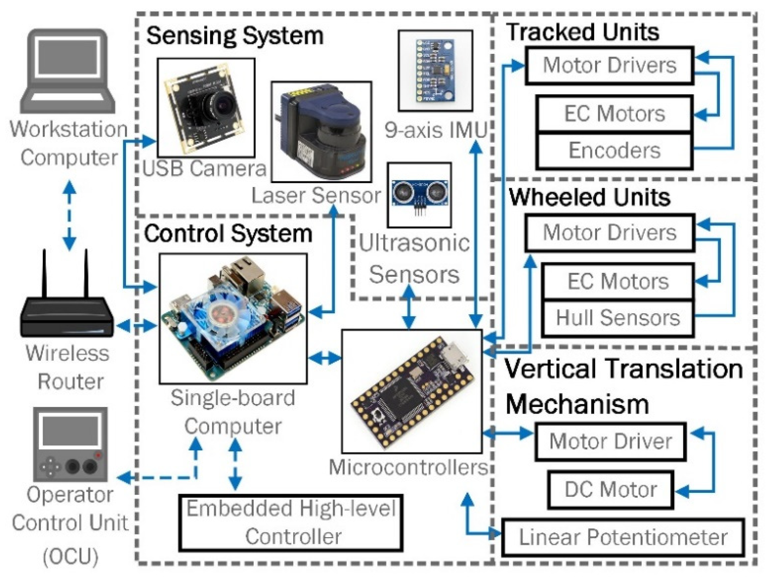
4.2. Electronic System

The electronic system is designed to enable the robot to perform the diverse tasks. The electronic hardware architecture is presented in Figure 5.
The internal electronic system can be divided into three subsystems: control, sensing, and actuation. All the components built-in or mounted on the robot platform are shown inside the dashed line (Figure 5), classified as the internal hardware group. A workstation computer and a wireless router belong to the external hardware group. Optionally, an Operator Control Unit (OCU), such as a joystick, is able to control the motions of the robot module via Bluetooth. The core of the mobile robot is the control system which contains a single-board computer (ODROID-XU4) and two microcontrollers (TEENSY 2.0). The ODROID-XU4 has an ARM CPU and 2 GB of high-speed RAM. The TEENSY 2.0 microcontroller has an 8-Bit AVR Processor running at 16 MHz (ATMEGA32U4). The electronic control system is in charge of sending commands, acquiring sensor data and communicating with the external hardware or other robots if required. The main components of the actuation system are five motors. Each tracked unit is actuated by a high-torque Maxon EC motor with an encoder. Maxon Flat EC motors with hall sensors drive the wheeled units. A DC motor is used to drive the VTM to provide vertical mobility. A potentiometer is attached to monitor the position of the VTM and gives feedback to a PID controller for precise height control. The sensing system has four ultrasonic sensors, two USB cameras, a Hokuyo LIDAR, and a 9-axis motion tracking device. The LIDAR is mounted on top of the VTU to assist with autonomous navigation.

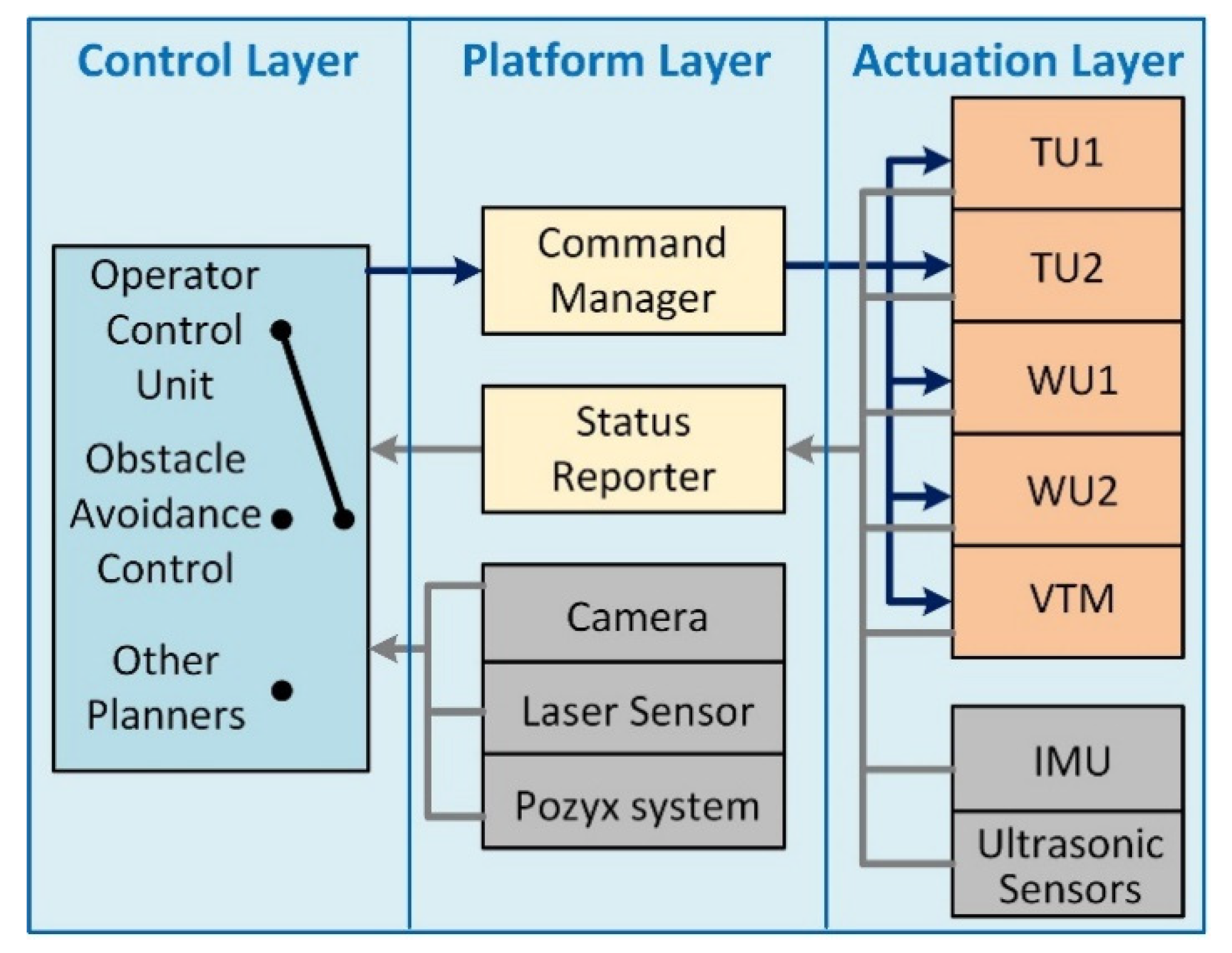
4.3. Software System

A three-layer software architecture is designed to manage different controllers for various subtasks of the STORM system. These controllers can be developed in parallel without the complete knowledge of the software architecture, such as the previously developed autonomous docking controller [16], the path planner [14], and the trajectory tracking controller [15].
The software architecture is developed in a publish-subscribe pattern based on Robot Operating System (ROS). As shown in Figure 6, the software architecture consists of three layers: the actuation layer, the platform layer, and the control layer. This architecture divides the overall software system into smaller modules. This feature, together with the publish-subscribe pattern, enables modular design and parallel development.
The software in the actuation layer is embedded in the microcontroller. The commands from the higher-level controllers can be published to the command manager in the platform layer. The command manager converts it into 8-bit unsigned integer array for sending the enable signal for each of the individual sensors as well as speed information for the motors. All the components in the actuation layer are programmed as state machines operating on the commands from the command manager. They transit between standby and execution states based on the commands.
Due to the different properties of the various sensors, the software for the sensing system is separated into the actuation layer and the platform layer. The ultrasonic sensors, potentiometer, and the 9-axis IMU are interfaced with the microcontrollers. The raw data from these sensors are published to the status reporter together with the feedback information about the motors. The cameras, LIDAR, and an optional localization device named Pozyx [37] are directly connected to the single-board computer. The software processes to interface these sensors are in the platform layer. Each sensor publishes out a topic for acquiring and sending the raw data. The high-level controllers can then subscribe to the status reporter and the sensor topics for any required information.
All the software in the platform layer and the actuation layer is designed to be reusable. The implementation of the control layer represents the extensible nature of the software architecture. The architecture allows for different control methods to be developed in parallel. Each method can choose the required information provided by the status reporter and the sensor processes running on the single-board computer. It is possible that some high-level controllers may require more computing power than what is provided by the single-board computer. For instance, the neural network in the proposed obstacle avoidance approach cannot be implemented on the single-board computer. Instead, it is implemented on a workstation, and the platform layer is made to subscribe to the topics published by the workstation through ROS.

5. Simulations and Results

To train and test the neural network, various simulation environments and a virual STORM locomotion module were developed in Gazebo simulator [10]. It is critical to map the obtained linear and angular velocities from the high-level commands to the velocities of each track or wheel of the STORM locomotion module in the simulation as well as in the real-world experiments. As such, a skid-steering kinematic model of the STORM locomotion module was developed and presented in the following subsection.

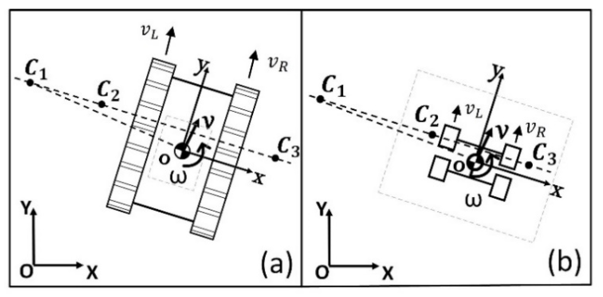
5.1. Kinematic Model of the Virtual STORM Module

The locomotion module can be regarded as a tracked mobile robot when the VTU is lifted. When the VTU is lowered, the robot is considered to be in wheeled mobile robot mode. However, in both cases, it operates as a skid-steer mobile robot, as shown in Figure 7. The kinematics for this system can be represented as follows:
( v L , v R ) = f ( v , ω )
where v = ( v x , v y ) is the linear velocity of the robot; v x and v y are the components of v along the X and Y axes, respectively; ω is the angular velocity of the robot; v L and v R are the linear velocity of the left and right tracked or wheeled mobility unit with respect to the local frame of reference.
Any planar movement of a rigid body can be regarded as a rotation about a single point, defined as the instantaneous center of rotation (ICR). The skid-steer mobile robot during a turning maneuver can be considered as a rigid body that is rotating about its ICR. The ICRs of the left and right treads are different from the ICR of the body of the robot. According to the Kennedy’s Theorem, all three ICRs have to be aligned in a straight line [38]. In Figure 7, C 1 = ( x c 1 , y c 1 ) is the ICR of the STORM locomotion module, and C 2 = ( x c 2 , y c 2 ) and C 3 = ( x c 3 , y c 3 ) are the ICRs of the left and right wheeled or tracked units, respectively.
Based on the calculated ICRs, the linear velocities of the robot can be calculated as follows:
v L = | x c 2 | ω + v y v R = | x c 3 | ω + v y
In the above model, the local x coordinates x c 2 and x c 3 were estimated via experiments in simulation. Known values of v L and v R were given to the robot and the resulting ω and v y . Using Equation (8), the average values of x c 2 and x c 3 were calculated from the recorded data. The estimated values are as follows: in the tracked mobility mode, | x c 2 | = 0.29 m and | x c 3 | = 0.3 m, in the wheeled mobility mode, | x c 2 | = 0.14 m, and | x c 2 | = 0.15 m.
With the knowledge of the kinematic relations of the locomotion module, the virtual STORM module with a 2D laser scanner was simulated in Gazebo, as shown in Figure 8. The LIDAR takes 512 measurements in a 270° span. A set of 50 range measurements are selected evenly from the sensor. The distance measurements are preprocessed to fall within a range of 0.00 m to 5.00 m.
The sensor data and state information were obtained from the simulator and then provided to the neural network as inputs. The commands to the virtual robot were sent based on the outputs of the neural network. Communication was done through publishing and subscribing to ROS topics.
The proposed collision avoidance method is general in the sense that it can be applied to both the tracked mobility mode and wheeled mobility mode of the locomotion module. The trainings and experiments in both the simulation environments and real-world implementation were conducted with the robot in the tracked mode.

5.2. Training Parameter Selection and Analysis

The proposed approach uses ε-greedy policy to choose the appropriate action. This policy allows the selection of a random action with probability ε. Otherwise, the robot will select the action with the highest value from the neural network. At the beginning of the training, ε is set to 1 , and the robot always selects a random action to acquire varied training data for updating the neural network. This is defined as the exploration stage. However, the robot cannot always select a random action, as it also needs to exploit the actions. With a probability of ( 1 ε ) , the robot will follow the output of the current neural network and choose the action with the highest value in the current state. If the robot can receive a similar reward to what it gets in the recorded transitions, the neural network is understood as well-trained. If not, the neural network needs more data to exploit. The decay rate β of the probability ε is used for balancing the exploration and the exploitation. A lower β means that the robot chooses fewer random actions when it meets the same environment state. It relies more on the previous experiences it had already obtained. The value of β will stop decaying after it reaches 0.05, which means that the robot will end up choosing a random action with a probability of 5%. To demonstrate the inferences of the parameters β and ε, as well as to evaluate the performances of the virtual STORM, a test of the virtual robot was set up in the simulation as follows:
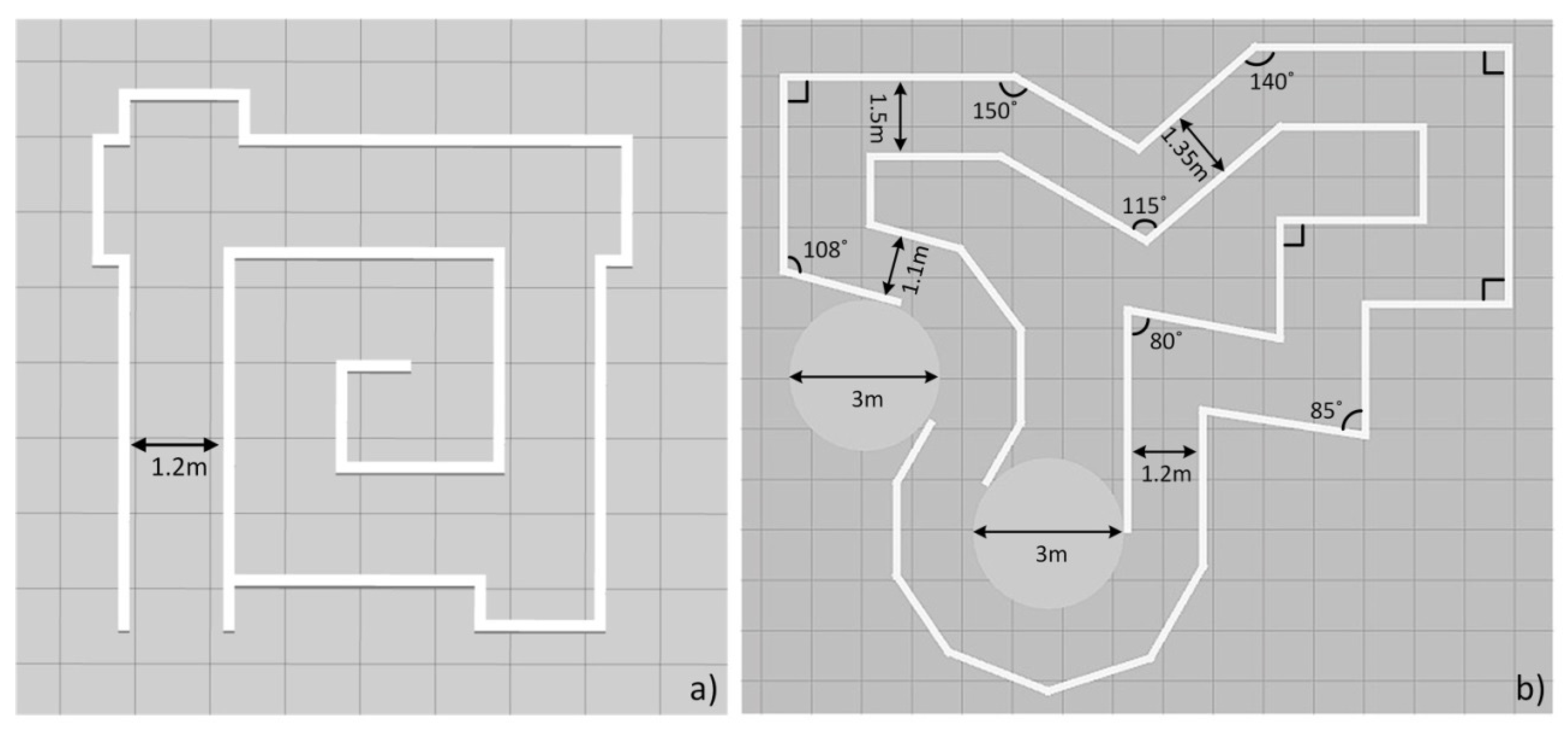
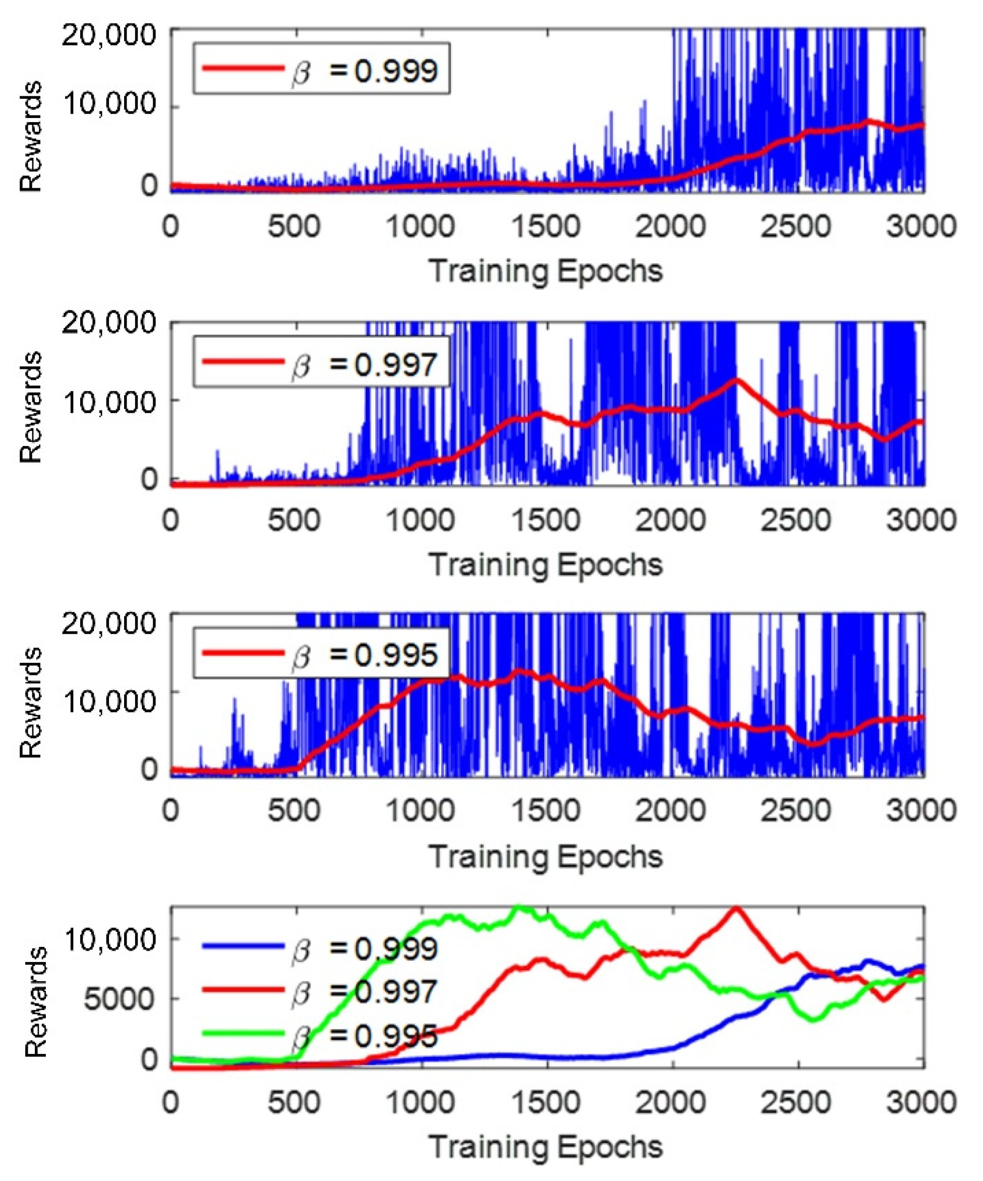
  • The training process was performed three times in Map 2, as shown in Figure 9b, with the decay rate β set to 0.997, 0.998, and 0.999, respectively. Each neural network was trained for 3000 epochs for the following reasons: (a) All the three tests reach the lowest value of ε to choose a random action after 3000 epochs, for example, when β = 0.999, ε reaches 0.05 at log 0.999 0.05 = 2994 epochs. (b) The current work did not include the improvement of the training efficiency. Training the neural network for 3000 epochs keeps the entire test within an acceptable training time, while at the same time ensuring that reasonable results can be obtained according to our previous experiences when training the neural network in [32].
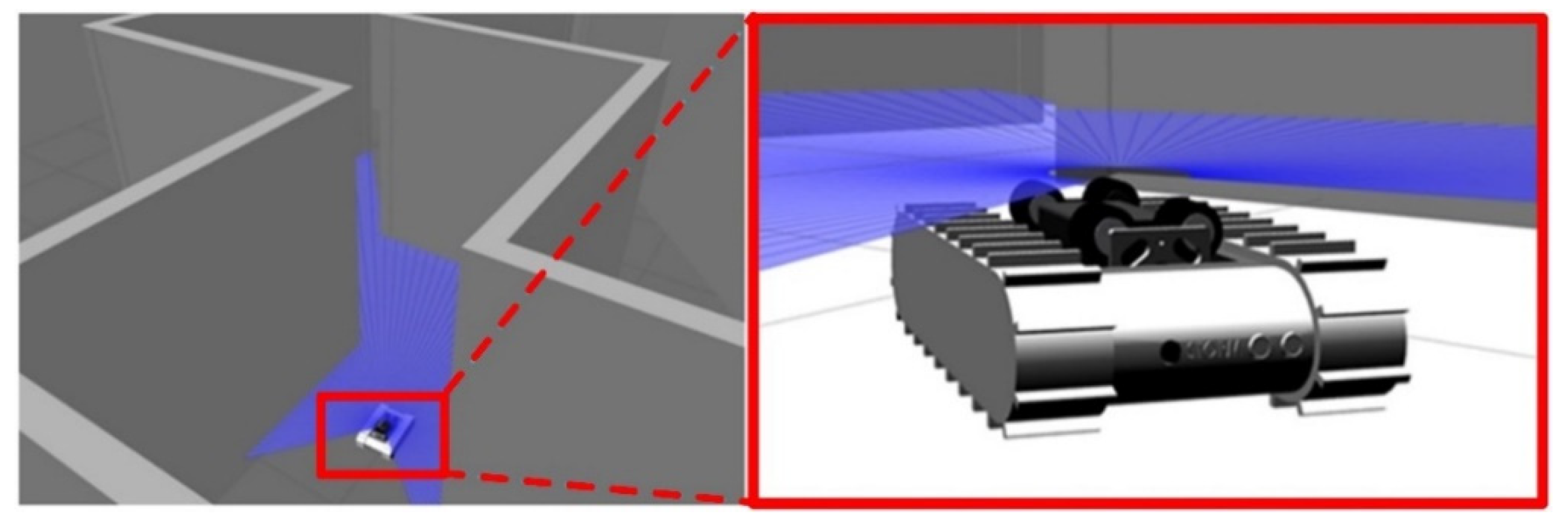
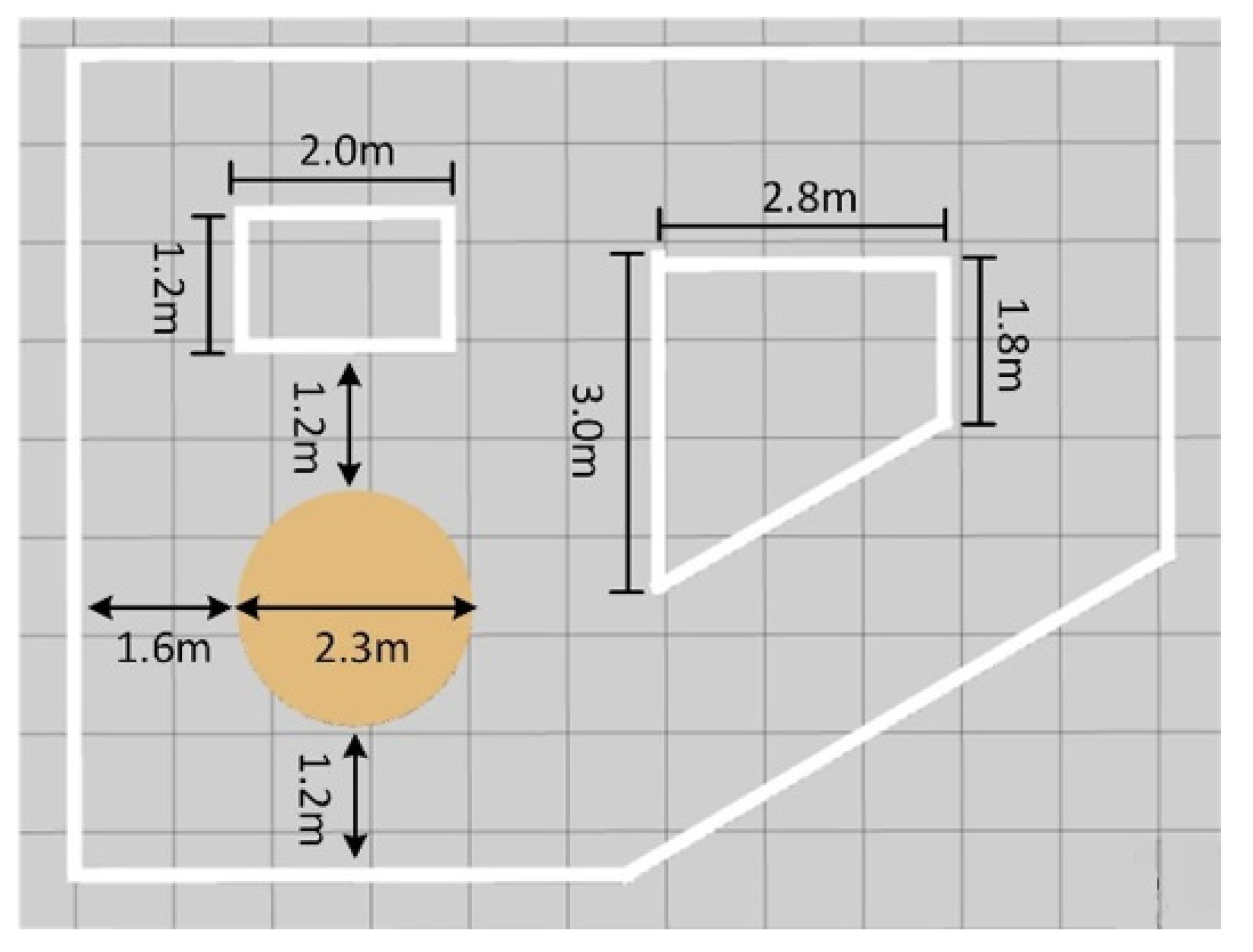
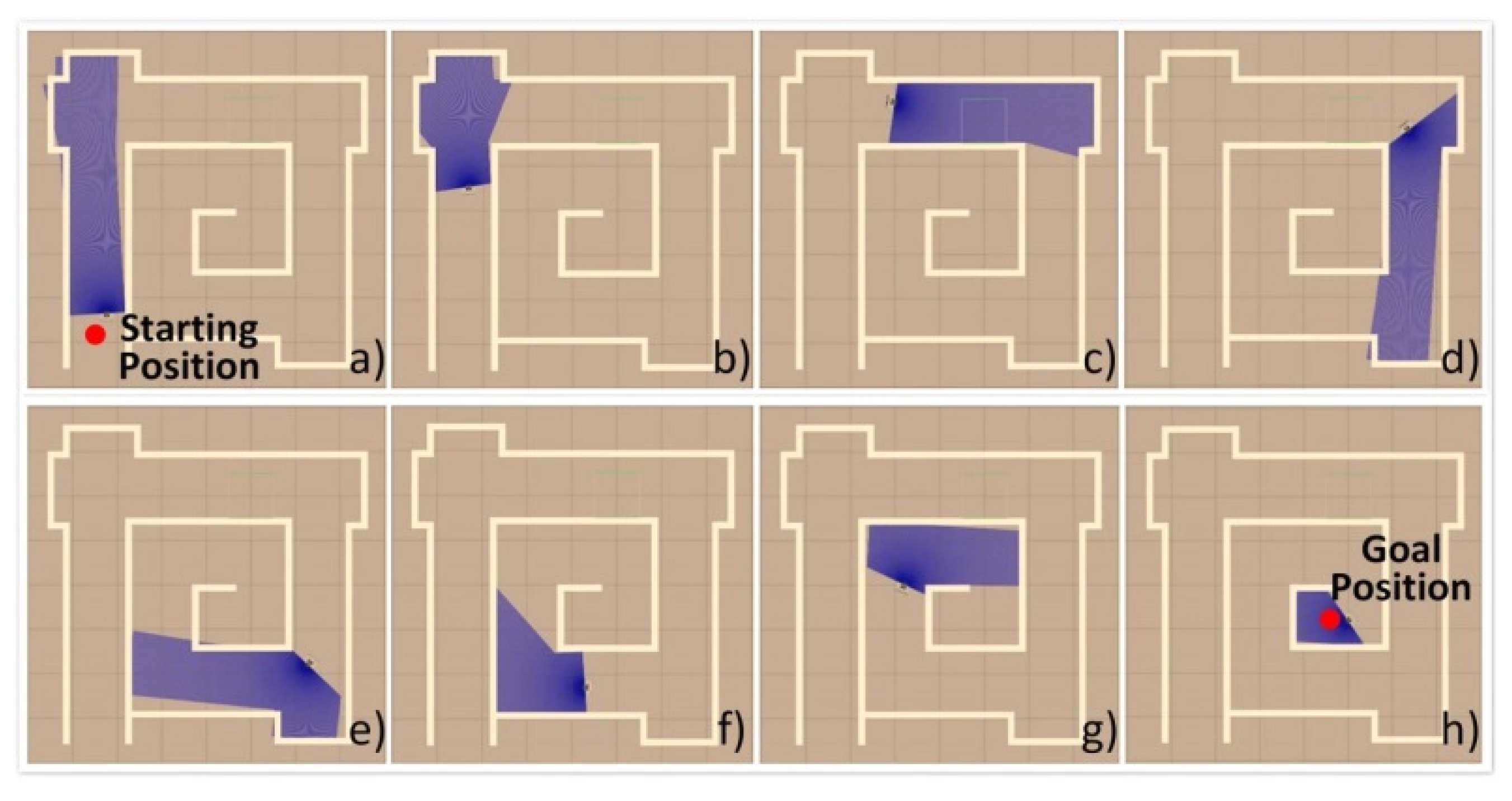
  • The three neural networks were applied to the virtual STORM successively to navigate the test map with similar features in Map 2, as shown in Figure 10, for five minutes. The metric for evaluating the performance of the neural networks is chosen to be the number of collisions undergone within five minutes of simulation.

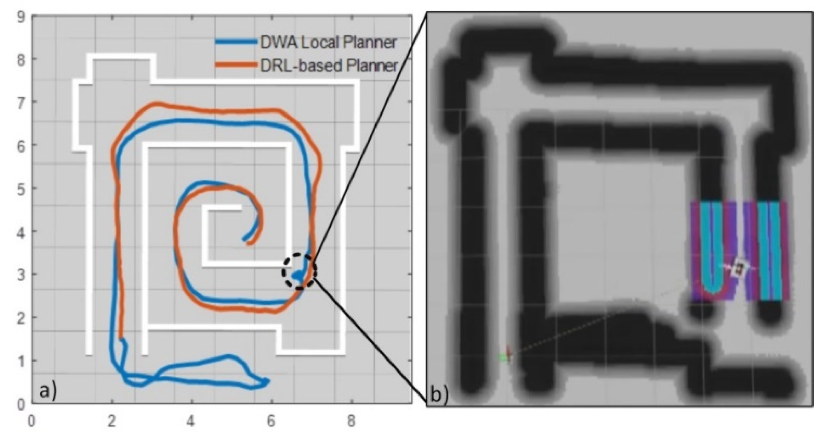
5.3. Comparison with State-of-the-Art Method

To demonstrate the advantages of the proposed DRL based planner, it was compared with the DWA local planner [30] in the virtual world, as shown in Figure 9a. There are mainly two reasons why this map was developed. The first one is to serve as the testbed for comparing the proposed method with the dynamic window-based method. The second one is to address the problem state in the introduction (Figure 1) by adding features in each corner of the map, which aims to demonstrate that the proposed method has the ability to avoid the problem mentioned in the introduction section.
The proposed method allows the robot to avoid obstacles based on the information from the sensor directly. In contrast, the DWA local planner is based on a dynamic window approach. Besides the data from the laser sensor, a cost map, generated according to odometry information, is required for the DWA planner to predict the safe motion. The feasibility of the path from the DWA local planner relies very much on the precision of the provided costmap. This is especially true in the case when the robot is navigating through narrow passageways. Consequently, the drift in odometer data may cause collisions under the DWA local planner. As such, the proposed method is superior to the DWA planner since it only relies on the sensor data as input.

5.4. Simulation Results

The results of the simulation are summarized and analyzed in this section. Figure 11 shows the training results to compare the performances of the neural network with different decay rates.
From the results, it can be observed that with a lower value of β in Equation (3), the neural network tended to get higher rewards fast. However, the rewards obtained during the training with a low value of β were not stable. This is because the robot chose an action with the highest Q-value according to the current neural network with a high probability. Nevertheless, this action was overestimated in the beginning due to insufficient experiences acquired at that time. The Q-value of that action decreased with more exploitations. A higher value of β caused the robot to explore more actions at first. This allowed the robot to take different actions when it met the same situation to determine which one was better. The reward curves show that the learning process with the highest β was slow but stably increased. It should be pointed out that the robot cannot achieve the highest score by navigating the training map for one round without any collisions, as shown in the results, because it still had the learning capabilities by selecting a random action with a probability of 5%. However, after training, the robot with each neural network was able to navigate the training map without collisions when it took action with the highest values according to the outputs of that neural network without the probabilities of choosing random actions. In conclusion, a higher decaying rate of the probability of choosing a random action causes the robot to learn fast, but the value of the actions as the outputs of the neural networks was not stable. One can decrease the value of β to evaluate if the actions that are already learned are proper or not. One can decrease the value of β to obtain more stable results on the account of longer training time.
The performance of the robot with different neural networks over a duration of five minutes in the test map differs from the test map shown in Table 3. It proved that the DRL-based obstacle avoidance method has the potential to deal with similar situations it had already learned. Further tests of the robustness of the proposed controller were conducted in the real world.
Figure 12 shows a sequence of frames captured from the simulated environment with a virtual STORM locomotion module under the DRL-based obstacle avoidance controller. For the simulated case, the virtual robot maneuvers through the narrow corridor-like maze successfully without any collisions. In comparison, another sequence of frames captured from the simulation is shown in Figure 13 with the locomotion module under the DWA local planner. The trajectories of the robot under the action of the two different planners are compared in Figure 14. As seen from Figure 13b, the robot goes out of the maze due to the lack of environmental information in order to plan a global path in advance. After a recovery behavior, the robot comes up with a new plan and goes in the correct direction, as shown in Figure 13c,d. It should be noted that at one of the corners of the maze, as shown in Figure 13e,f, the robot almost bumped into the wall and failed to come up with a reliable local path. The reason is that the costmap generated from the odometer data was not precise at that specific time step, as shown in Figure 14b. This causes the robot to spin around and collect more information and thereby plan a new path. In conclusion, the proposed DRL-based method is capable of planning a proper motion for the mobile robot solely based on the data collected from the laser sensor directly. This in turn reduces the inaccuracy caused by other processes, such as costmap generation.

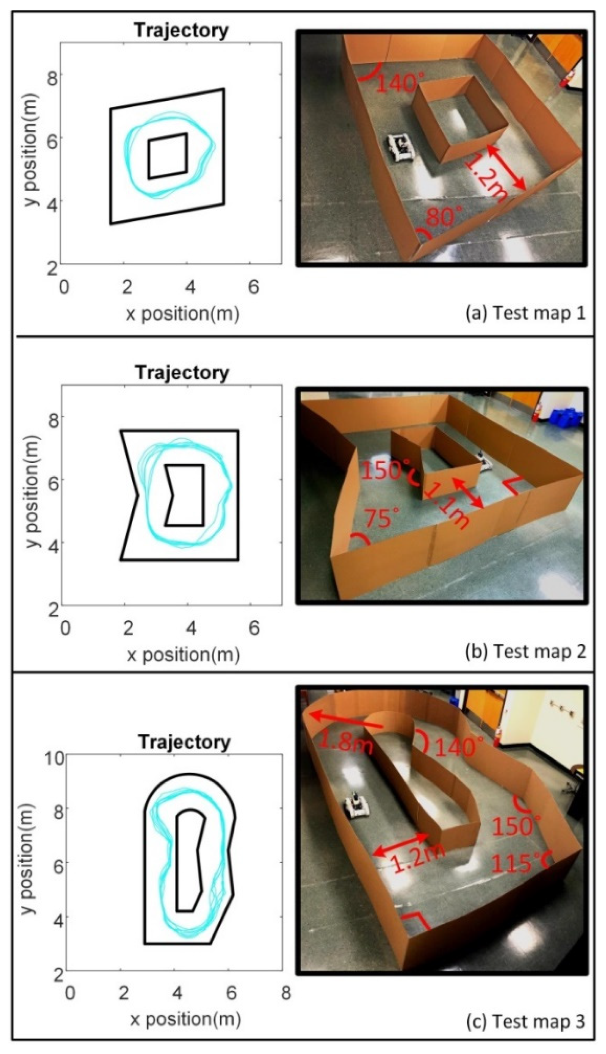
5.5. Real-World Implementation

The obstacle avoidance controller for the STORM prototype was embedded in the control layer. The neural network trained with β = 0.999 was selected as it offered the best performance. As mentioned before, the trained neural network was made to run on a workstation since it was beyond the computational power of the onboard single board computer. The neural network generated the command a i = ( v , ω m ) with an update rate of 10 Hz. These commands were subscribed by the command manager on board STORM locomotion module and converted into the proper form for the actuation layer.
As mentioned before, the neural network found optimal actions based on the sensor observations in the simulated world, but the map was the same as that used for training. In order to validate the ability of the robot to travel without collisions, not only in the same map as the training case but also in environments with different features, three maps different from the training scenarios were built to test the robot. One of the maps had a circular feature with different diameters as compared to the simulated training environment. Figure 15 shows the three test maps and the trajectories followed by the robot when traveling through the maps. The robot traveled in each of the three maps for five minutes without collision. This proved that the proposed approach could handle situations different from the training scenario provided in the 3D simulation.

6. Conclusions and Future Work

The DRL-based method shows the potential to improve the performance of the robot when avoiding obstacles in some highly occupied environments and problematic scenarios. The proposed DRL architecture was trained inside a simulated Gazebo environment to allow for sufficient data collection over varied features without any damage to the real robot. The results from the simulations show that more exploration in training leads to stably increased rewards with slow training speed. The trained DRL architecture was tested in real-world scenarios with the STORM locomotion module. The experimental results show that the proposed approach was able to perform well in previously unseen scenarios that are much different from the training scenario, thereby proving a generalized nature of the trained architecture.
Future work will incorporate a specified goal position without a prior map, along with obstacle avoidance capabilities. The maps developed in the Gazebo simulator aimed to emphasize the compact spaced environment and problematic scenarios. The training environment should be more complex and involve various features to enable robust performances of the robot. Further training and investigations will include a multi-stage training with a shared memory set and maps of gradually increased difficulty, in contrast to learning directly from the complex environments. Besides, the training efficiency will be taken into consideration when improving the proposed obstacle avoidance methods. To a larger extent, this work is a step forward in enabling multi-robot exploration and navigation in unknown environments for the STORM system. As part of future work, new simulation environments with moving obstacles and uneven terrain will be considered to enrich the experience of the trained neural network.

Author Contributions

Methodology, S.F.; project administration, P.B.-T.; supervision, P.B.-T.; validation, S.F.; writing—original draft, S.F.; writing—review and editing, B.S. and P.B.-T. All authors have read and agreed to the published version of the manuscript.

Funding

This research received no external funding.

Institutional Review Board Statement

Not applicable.

Informed Consent Statement

Not applicable.

Conflicts of Interest

The authors declare no conflict of interest.

References

  1. Silver, D.; Hubert, T.; Schrittwieser, J.; Antonoglou, I.; Lai, M.; Guez, A.; Lanctot, M.; Sifre, L.; Kumaran, D.; Graepel, T.; et al. Mastering chess and shogi by self-play with a general reinforcement learning algorithm. arXiv 2017, arXiv:1712.01815. [Google Scholar]
  2. François-Lavet, V.; Henderson, P.; Islam, R.; Bellemare, M.G.; Pineau, J. An Introduction to Deep Reinforcement Learning. Found. Trends Mach. Learn. 2018, 11, 219–354. [Google Scholar] [CrossRef] [Green Version]
  3. Moreira, I.; Rivas, J.; Cruz, F.; Dazeley, R.; Ayala, A.; Fernandes, B. Deep reinforcement learning with interactive feedback in a human-robot environment. Appl. Sci. 2020, 10, 5574. [Google Scholar] [CrossRef]
  4. Gu, S.; Holly, E.; Lillicrap, T.; Levine, S. Deep reinforcement learning for robotic manipulation with asynchronous off-policy updates. In Proceedings of the 2017 IEEE International Conference on Robotics and Automation (ICRA), Singapore, 29 May–3 June 2017; IEEE: Piscataway, NJ, USA, 2017; pp. 3389–3396. [Google Scholar] [CrossRef] [Green Version]
  5. Pirník, R.; Hruboš, M.; Nemec, D.; Mravec, T.; Božek, P. Integration of inertial sensor data into control of the mobile platform. Adv. Intell. Syst. Comput. 2017, 511, 271–282. [Google Scholar]
  6. Kilin, A.; Bozek, P.; Karavaev, Y.; Klekovkin, A.; Shestakov, V. Experimental investigations of a highly maneuverable mobile omniwheel robot. Int. J. Adv. Robot. Syst. 2017, 14, 1–9. [Google Scholar] [CrossRef]
  7. Zhu, Y.; Mottaghi, R.; Kolve, E.; Lim, J.J.; Gupta, A.; Fei-Fei, L.; Farhadi, A. Target-driven visual navigation in indoor scenes using deep reinforcement learning. In Proceedings of the 2017 IEEE International Conference on Robotics and Automation (ICRA), Singapore, 29 May–3 June 2017; IEEE: Piscataway, NJ, USA, 2017; Volume 1, pp. 3357–3364. [Google Scholar]
  8. Tai, L.; Paolo, G.; Liu, M. Virtual-to-real deep reinforcement learning: Continuous control of mobile robots for mapless navigation. In Proceedings of the 2017 IEEE/RSJ International Conference on Intelligent Robots and Systems (IROS), Vancouver, BC, Canada, 24–28 September 2017; IEEE: Piscataway, NJ, USA, 2017; pp. 31–36. [Google Scholar]
  9. Ulrich, I.; Borenstein, J. VFH*: Local obstacle avoidance with look-ahead verification. In Proceedings of the Proceedings 2000 ICRA. Millennium Conference. IEEE International Conference on Robotics and Automation. Symposia Proceedings (Cat. No.00CH37065), San Francisco, CA, USA, 24–28 April 2000; IEEE: Piscataway, NJ, USA, 2000; Volume 3, pp. 2505–2511. [Google Scholar]
  10. Gazebo. Available online: http://gazebosim.org/ (accessed on 12 May 2017).
  11. Kumar, P.; Saab, W.; Ben-Tzvi, P. Design of a Multi-Directional Hybrid-Locomotion Modular Robot With Feedforward Stability Control. In Proceedings of the Volume 5B: 41st Mechanisms and Robotics Conference, Cleveland, OH, USA, 6–9 August 2017; ASME: New York, NY, USA, 2017; p. V05BT08A010. [Google Scholar] [CrossRef] [Green Version]
  12. Ben-Tzvi, P.; Saab, W. A hybrid tracked-wheeled multi-directional mobile robot. J. Mech. Robot. 2019, 11, 1–10. [Google Scholar] [CrossRef] [Green Version]
  13. Moubarak, P.M.; Alvarez, E.J.; Ben-Tzvi, P. Reconfiguring a modular robot into a humanoid formation: A multi-body dynamic perspective on motion scheduling for modules and their assemblies. In Proceedings of the 2013 IEEE International Conference on Automation Science and Engineering (CASE), Madison, WI, USA, 17–21 August 2013; IEEE: Piscataway, NY, USA, 2013; pp. 687–692. [Google Scholar] [CrossRef]
  14. Sebastian, B.; Ben-Tzvi, P. Physics Based Path Planning for Autonomous Tracked Vehicle in Challenging Terrain. J. Intell. Robot. Syst. Theory Appl. 2018, 1–16. [Google Scholar] [CrossRef]
  15. Sebastian, B.; Ben-Tzvi, P. Active Disturbance Rejection Control for Handling Slip in Tracked Vehicle Locomotion. J. Mech. Robot. 2018, 11, 021003. [Google Scholar] [CrossRef] [Green Version]
  16. Sohal, S.S.; Saab, W.; Ben-Tzvi, P. Improved Alignment Estimation for Autonomous Docking of Mobile Robots. In Proceedings of the Volume 5A: 42nd Mechanisms and Robotics Conference, Quebec City, QC, Canada, 26–29 August 2018; ASME: New York, NY, USA, 2018; p. V05AT07A072. [Google Scholar] [CrossRef]
  17. Hart, P.; Nilsson, N.; Raphael, B. A Formal Basis for the Heuristic Determination of Minimum Cost Paths. IEEE Trans. Syst. Sci. Cybern. 1968, 4, 100–107. [Google Scholar] [CrossRef]
  18. Lozano-Pérez, T.; Wesley, M.A. An Algorithm for Planning Collision-Free Paths Among Polyhedral Obstacles. Commun. ACM 1979, 22, 560–570. [Google Scholar] [CrossRef]
  19. Khatib, O. Real-Time Obstacle Avoidance for Manipulators and Mobile Robots. Int. J. Rob. Res. 1986, 5, 90–98. [Google Scholar] [CrossRef]
  20. Brock, O.; Khatib, O. High-speed navigation using the global dynamic window approach. In Proceedings of the Proceedings 1999 IEEE International Conference on Robotics and Automation (Cat. No.99CH36288C), Detroit, MI, USA, 10–15 May 1999; IEEE: Piscataway, NJ, USA, 1999; Volume 1, pp. 341–346. [Google Scholar]
  21. Koren, Y.; Borenstein, J. Potential field methods and their inherent limitations for mobile robot navigation. In Proceedings of the Proceedings. 1991 IEEE International Conference on Robotics and Automation, Sacramento, CA, USA, 7–12 April 1991; IEEE: Piscataway, NJ, USA, 2016; Volume 11, pp. 1398–1404. [Google Scholar]
  22. Borenstein, J.; Koren, Y. The vector field histogram-fast obstacle avoidance for mobile robots. IEEE Trans. Robot. Autom. 1991, 7, 278–288. [Google Scholar] [CrossRef] [Green Version]
  23. Faisal, M.; Hedjar, R.; Al Sulaiman, M.; Al-Mutib, K. Fuzzy logic navigation and obstacle avoidance by a mobile robot in an unknown dynamic environment. Int. J. Adv. Robot. Syst. 2013, 10, 37. [Google Scholar] [CrossRef]
  24. Pothal, J.K.; Parhi, D.R. Navigation of multiple mobile robots in a highly clutter terrains using adaptive neuro-fuzzy inference system. Rob. Auton. Syst. 2015, 72, 48–58. [Google Scholar] [CrossRef]
  25. Dijkstra, E.W. A note on two problems in connexion with graphs. Numer. Math. 1959, 1, 269–271. [Google Scholar] [CrossRef] [Green Version]
  26. Dechter, R.; Pearl, J. Generalized Best-First Search Strategies and the Optimality of A. J. ACM 1985, 32, 505–536. [Google Scholar] [CrossRef]
  27. Kavraki, L.E.; Svestka, P.; Latombe, J.-C.; Overmars, M.H. Probabilistic roadmaps for path planning in high-dimensional configuration spaces. IEEE Trans. Robot. Autom. 1996, 12, 566–580. [Google Scholar] [CrossRef] [Green Version]
  28. Elbanhawi, M.; Simic, M. Sampling-based robot motion planning: A review. IEEE Access 2014, 2, 56–77. [Google Scholar] [CrossRef]
  29. Ulrich, I.; Borenstein, J. VFH+: Reliable obstacle avoidance for fast mobile robots. Proc. IEEE Int. Conf. Robot. Autom. 1998, 2, 1572–1577. [Google Scholar]
  30. Haarnoja, T.; Pong, V.; Zhou, A.; Dalal, M.; Abbeel, P.; Levine, S. Composable deep reinforcement learning for robotic manipulation. arXiv 2018, arXiv:1803.06773v1. [Google Scholar]
  31. Wang, C.; Wang, J.; Shen, Y.; Zhang, X. Autonomous Navigation of UAVs in Large-Scale Complex Environments: A Deep Reinforcement Learning Approach. IEEE Trans. Veh. Technol. 2019, 68, 2124–2136. [Google Scholar] [CrossRef]
  32. Feng, S.; Ren, H.; Wang, X.; Ben-Tzvi, P. Mobile robot obstacle avoidance base on deep reinforcement learning. Proc. ASME Des. Eng. Tech. Conf. 2019, 5A-2019, 1–8. [Google Scholar]
  33. Sutton, R.S.; Barto, A.G. Chapter 1 Introduction. Reinf. Learn. An Introd. 1988. [Google Scholar] [CrossRef]
  34. Mnih, V.; Kavukcuoglu, K.; Silver, D.; Graves, A.; Antonoglou, I.; Wierstra, D.; Riedmiller, M. Playing Atari with Deep Reinforcement Learning. arXiv 2013, arXiv:1312.5602. [Google Scholar]
  35. Van Hasselt, H.; Guez, A.; Silver, D. Deep Reinforcement Learning with Double Q-learning. Assoc. Adv. Artif. Intell. 2016, 30, 2094–2100. [Google Scholar]
  36. Saab, W.; Ben-Tzvi, P. A Genderless Coupling Mechanism with 6-DOF Misalignment Capability for Modular Self-Reconfigurable Robots. J. Mech. Robot. 2016, 8, 1–9. [Google Scholar] [CrossRef]
  37. POZYX Positioning System. Available online: https://www.pozyx.io/ (accessed on 23 February 2018).
  38. Mandow, A.; Martinez, J.L.; Morales, J.; Blanco, J.L.; Garcia-Cerezo, A.; Gonzalez, J. Experimental kinematics for wheeled skid-steer mobile robots. IEEE Int. Conf. Intell. Robot. Syst. 2007, 1222–1227. [Google Scholar] [CrossRef]
Figure 1. Robot in a narrow corridor. The blue circle indicates the trigger distance. Both A and B are the open areas detected by the autonomous robot at the current time step.
Robotics 10 00073 g001
Figure 2. Average q-values estimated by DQN, DDQN [32].
Robotics 10 00073 g002
Figure 3. Rewards from the training with Turtlebot employed DDQN and DDQN with PER, respectively [32].
Robotics 10 00073 g003
Figure 4. The architecture of the STORM locomotion module. The tracked unit, wheeled unit, and the vertical translational mechanism are indicated in the figure. (a) Tracked mobility mode. (b) Wheeled mobility. Note that the tracks are lifted by the vertical translational mechanism. (c) Various sensors that available on STORM.
Robotics 10 00073 g004
Figure 5. The electrical architecture of STORM.
Robotics 10 00073 g005
Figure 6. Software architecture: The various programs are divided into three different layers.
Robotics 10 00073 g006
Figure 7. Schematic figures of the locomotion module: (a) tracked mobility mode with ICR locations and (b) wheeled mobility with ICR locations are shown.
Robotics 10 00073 g007
Figure 8. Simulation environment. A virtual STORM locomotion module with a 2D range sensor in the simulation environment.
Robotics 10 00073 g008
Figure 9. The training maps. (a) Map 1: a simple corridor-like path with some problematic scenarios. (b) Map 2: a complex circuit with different environmental features such as straight tracks, 90-degree turns, and acute and obtuse angle corners.
Robotics 10 00073 g009
Figure 10. The test map with similar features to that in Map 2.
Robotics 10 00073 g010
Figure 11. Performance comparisons of the neural network with different decay rates: in the first three plots, the blue lines indicate the reward values, whereas the red line is the data processed by a moving average filter with a window size of 500. The blue, red, and green lines in the last plot stand for the trainings with different decay rates.
Robotics 10 00073 g011
Figure 12. STORM locomotion module with the proposed DRL-based planner initialized at (a) starting position, successfully passes the corners with special features shown in (b,d,e), and the corridors as shown in (c,f,g); finally goes to the goal position in the virtual environment.
Robotics 10 00073 g012
Figure 13. STORM locomotion module with the DWA local planner initialized at the (a) starting position goes out of the maze due to the lack of environmental information. In a recovery behavior, the robot comes up with a new plan and goes in the correct direction, as shown (bd). At one of the corners of the maze, as shown in (eg), the robot almost bumped into the wall and failed to come up with a reliable local path. It finally goes to the (h) goal position.
Robotics 10 00073 g013
Figure 14. (a) Comparison between the trajectories of the proposed DRL-based planner and the DWA local Planner. (b) The costmap feeds into the DWA planner at the moment the robot fails to produce a path.
Robotics 10 00073 g014
Figure 15. The test maps and the trajectories of the robot.
Robotics 10 00073 g015
Table 1. Comparison among path planning approach.
MethodsStrategyPrior Knowledge Real-Time CapabilityComments
A* [17]Search-based approachYesOffline planningAvoids expanding paths that are already expensive
Dijkstra’s Algorithm [25]Explores all the possible path and take more time
Greedy Best First Search [26]Finds out the optimal path fast but not always work
Probabilistic roadmap (PRM) [27]Sample-based planningYesOffline planningSelects a random node from the C-space and performs multi-query
RRT [28]Selects a random node from the C-space and incrementally adds new node
PF [19]Potential field-based approachNoOnline planningHas several drawbacks: local minima, no passage of narrow path, oscillations in narrow passages
VFF [21]Overcomes the local minima problem, but the other two shortcomings still exist
VFH [9], VFH+ [29]Overcomes the drawbacks, but problematic scenarios exist
VFH* [9]YesOvercomes the problematic scenarios but relies on information from a map
FLC [23] Fuzzy logic-based methodNoOnline planningGenerates various decisions according to different sensory information
Proposed ApproachDRL-based approachNoOnline planningGenerates optimal decisions from a well-trained neural network. Complex scenarios can be overcome as long as the robot has sufficient experiences during training
Table 2. Robot parameters.
CharacteristicParameters
Outer dimensions410 × 305 × 120 mm3
Vertical translation50 mm
Robot mass 8.40 kg
TU mass2 × 2.81 kg
WU mass2 × 0.76 kg
VTU0.73 kg
Table 3. Performance of obstacle avoidance approach.
Decay Rate βNumber of Collisions in 5 min
0.9990
0.9971
0.9952
Publisher’s Note: MDPI stays neutral with regard to jurisdictional claims in published maps and institutional affiliations.

