
Quantifying Yeast Microtubules and Spindles Using the Toolkit for Automated Microtubule Tracking (TAMiT)
Abstract
:1. Introduction
2. Materials and Methods
2.1. Mathematical Model
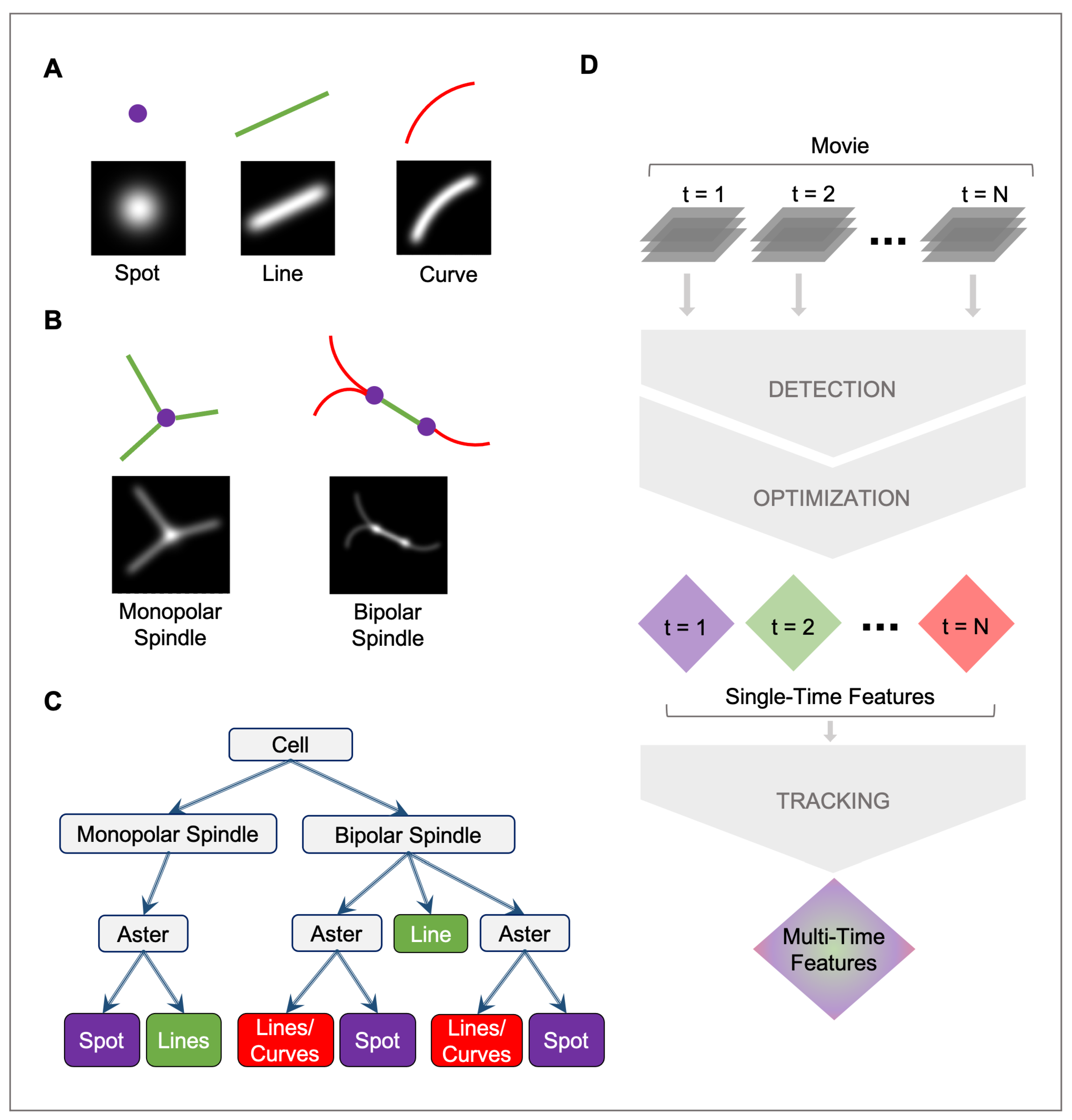
2.1.1. Spot
2.1.2. Line
2.1.3. Curve
2.2. Detection
2.3. Optimization
2.4. Tracking
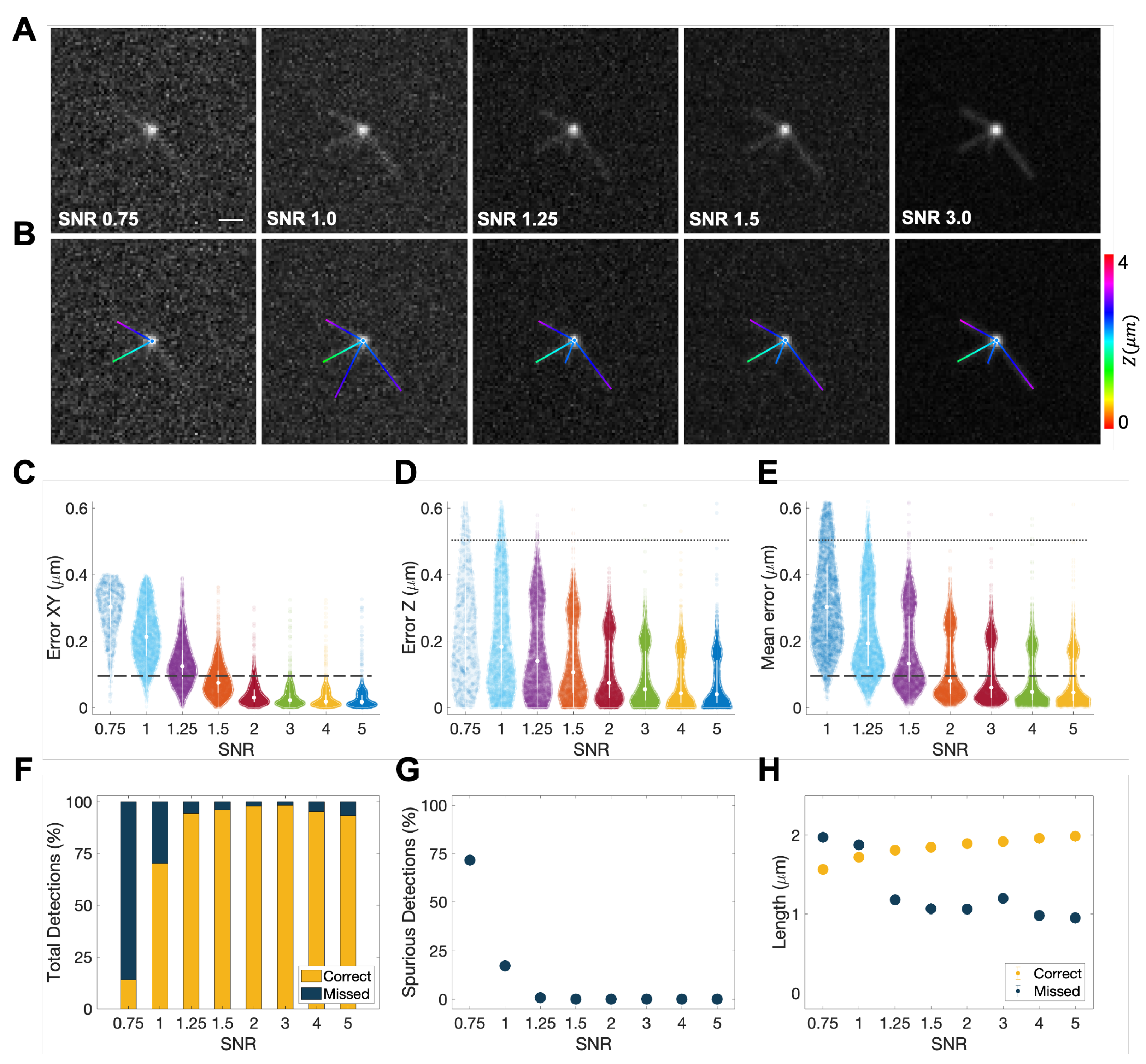
2.5. Validation
2.6. Experimental Methods
2.6.1. S. pombe
2.6.2. S. cerevisiae
2.7. Manual Analysis of Microtubule Dynamics in S. cerevisiae
3. Results
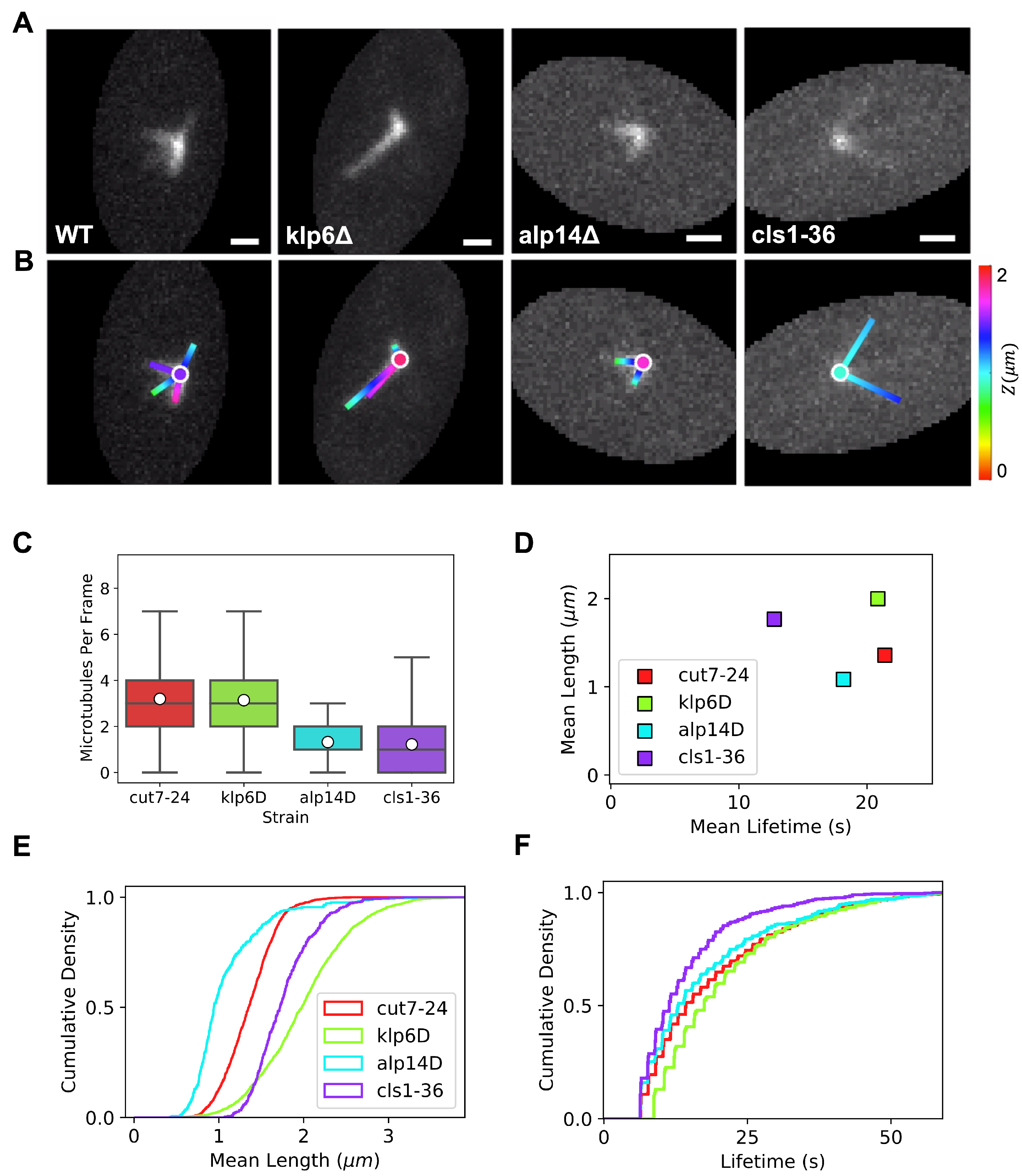
3.1. Quantification of Monopolar Spindle Microtubule Number, Length, and Lifetime
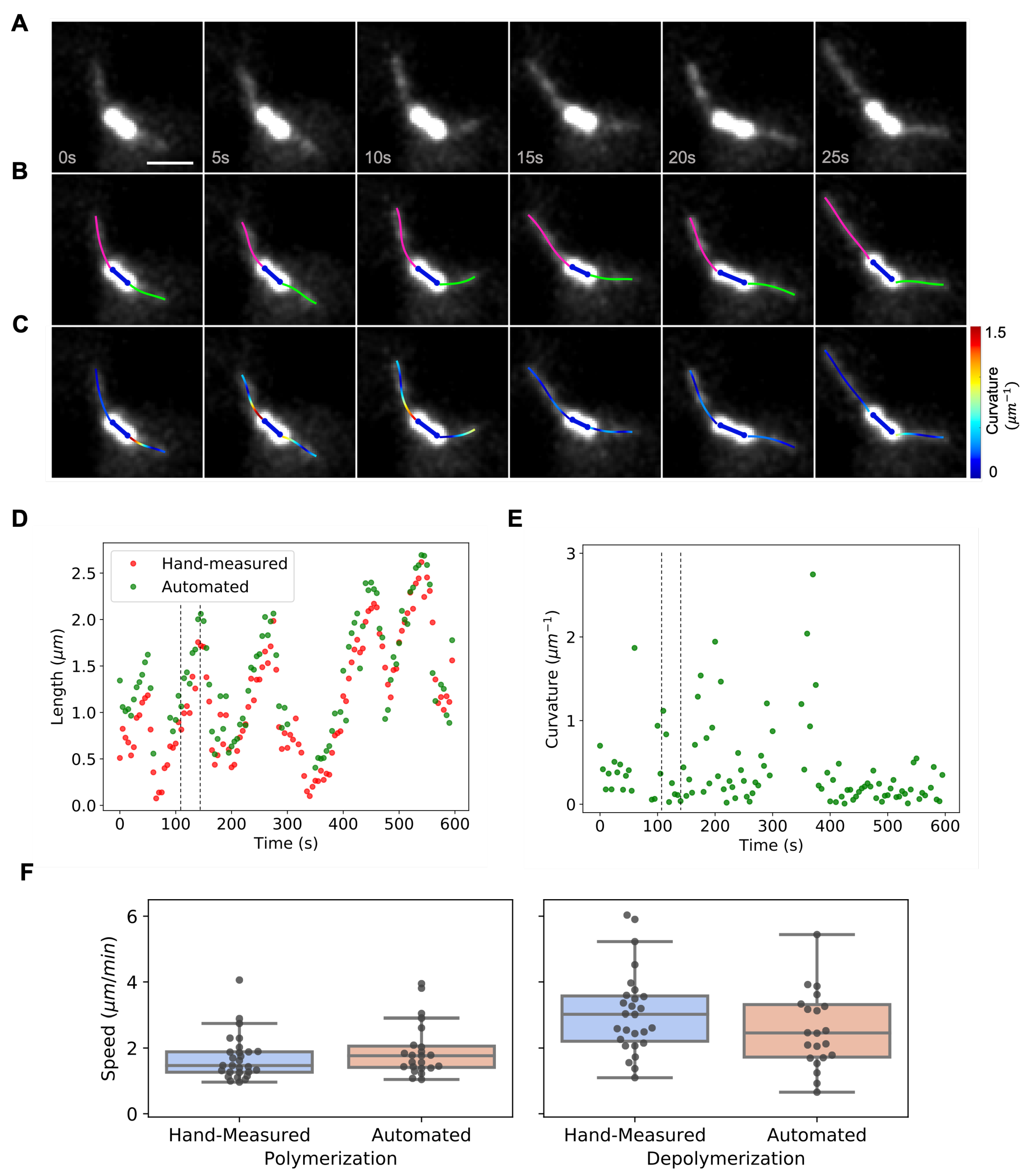
3.2. Dynamic Instability of Astral Microtubules in S. cerevisiae
4. Discussion
Supplementary Materials
Author Contributions
Funding
Institutional Review Board Statement
Informed Consent Statement
Data Availability Statement
Acknowledgments
Conflicts of Interest
References
- Zhang, B.; Zerubia, J.; Olivo-Marin, J.C. Gaussian approximations of fluorescence microscope point-spread function models. Appl. Opt. 2007, 46, 1819–1829. [Google Scholar] [CrossRef] [PubMed]
- Jaqaman, K.; Loerke, D.; Mettlen, M.; Kuwata, H.; Grinstein, S.; Schmid, S.L.; Danuser, G. Robust single-particle tracking in live-cell time-lapse sequences. Nat. Methods 2008, 5, 695–702. [Google Scholar] [CrossRef] [PubMed] [Green Version]
- Roudot, P.; Legant, W.R.; Zou, Q.; Dean, K.M.; Welf, E.S.; David, A.F.; Gerlich, D.W.; Fiolka, R.; Betzig, E.; Danuser, G. u-track 3D: Measuring and interrogating intracellular dynamics in three dimensions. bioRxiv 2020. [Google Scholar] [CrossRef]
- Gyori, B.M.; Venkatachalam, G.; Thiagarajan, P.; Hsu, D.; Clement, M.V. OpenComet: An automated tool for comet assay image analysis. Redox Biol. 2014, 2, 457–465. [Google Scholar] [CrossRef] [Green Version]
- Alberts, B.; Johnson, A.; Lewis, J.; Morgan, D.; Raff, M.; Roberts, K.; Walter, P. Essential Cell Biology: Fifth International Student Edition; WW Norton & Company: New York, NY, USA, 2018. [Google Scholar]
- Prosser, S.L.; Pelletier, L. Mitotic spindle assembly in animal cells: A fine balancing act. Nat. Rev. Mol. Cell Biol. 2017, 18, 187. [Google Scholar] [CrossRef]
- Caviston, J.P.; Holzbaur, E.L. Microtubule motors at the intersection of trafficking and transport. Trends Cell Biol. 2006, 16, 530–537. [Google Scholar] [CrossRef]
- Watanabe, T.; Noritake, J.; Kaibuchi, K. Regulation of microtubules in cell migration. Trends Cell Biol. 2005, 15, 76–83. [Google Scholar] [CrossRef]
- Wittmann, T.; Waterman-Storer, C.M. Cell motility: Can Rho GTPases and microtubules point the way? J. Cell Sci. 2001, 114, 3795–3803. [Google Scholar] [CrossRef]
- Kirschner, M.; Mitchison, T. Beyond self-assembly: From microtubules to morphogenesis. Cell 1986, 45, 329–342. [Google Scholar] [CrossRef]
- Baas, P.W.; Vidya Nadar, C.; Myers, K.A. Axonal transport of microtubules: The long and short of it. Traffic 2006, 7, 490–498. [Google Scholar] [CrossRef]
- Jordan, M.A.; Wilson, L. Microtubules as a target for anticancer drugs. Nat. Rev. Cancer 2004, 4, 253–265. [Google Scholar] [CrossRef]
- Kappes, B.; Rohrbach, P. Microtubule inhibitors as a potential treatment for malaria. Future Microbiol. 2007, 2, 4. [Google Scholar] [CrossRef]
- Kapoor, V.; Hirst, W.G.; Hentschel, C.; Preibisch, S.; Reber, S. MTrack: Automated detection, tracking, and analysis of dynamic microtubules. Sci. Rep. 2019, 9, 3794. [Google Scholar] [CrossRef] [Green Version]
- Ruhnow, F.; Zwicker, D.; Diez, S. Tracking single particles and elongated filaments with nanometer precision. Biophys. J. 2011, 100, 2820–2828. [Google Scholar] [CrossRef] [Green Version]
- Bohner, G.; Gustafsson, N.; Cade, N.I.; Maurer, S.; Griffin, L.; Surrey, T. Important factors determining the nanoscale tracking precision of dynamic microtubule ends. J. Microsc. 2016, 261, 67–78. [Google Scholar] [CrossRef] [Green Version]
- Xiao, X.; Geyer, V.F.; Bowne-Anderson, H.; Howard, J.; Sbalzarini, I.F. Automatic optimal filament segmentation with sub-pixel accuracy using generalized linear models and B-spline level-sets. Med. Image Anal. 2016, 32, 157–172. [Google Scholar] [CrossRef]
- Prahl, L.S.; Castle, B.T.; Gardner, M.K.; Odde, D.J. Quantitative analysis of microtubule self-assembly kinetics and tip structure. In Methods in Enzymology; Elsevier: Amsterdam, The Netherlands, 2014; Volume 540, pp. 35–52. [Google Scholar]
- Altinok, A.; Kiris, E.; Peck, A.J.; Feinstein, S.C.; Wilson, L.; Manjunath, B.; Rose, K. Model based dynamics analysis in live cell microtubule images. BMC Cell Biol. 2007, 8, S4. [Google Scholar] [CrossRef] [PubMed] [Green Version]
- Li, T.; Mary, H.; Grosjean, M.; Fouchard, J.; Cabello, S.; Reyes, C.; Tournier, S.; Gachet, Y. MAARS: A novel high-content acquisition software for the analysis of mitotic defects in fission yeast. Mol. Biol. Cell 2017, 28, 1601–1611. [Google Scholar] [CrossRef] [PubMed]
- Uzsoy, A.S.M.; Zareiesfandabadi, P.; Jennings, J.; Kemper, A.F.; Elting, M.W. Automated tracking of S. pombe spindle elongation dynamics. J. Microsc. 2020, 284, 83–94. [Google Scholar] [CrossRef] [PubMed]
- Perez, F.; Diamantopoulos, G.S.; Stalder, R.; Kreis, T.E. CLIP-170 highlights growing microtubule ends in vivo. Cell 1999, 96, 517–527. [Google Scholar] [CrossRef] [Green Version]
- Piehl, M.; Tulu, U.S.; Wadsworth, P.; Cassimeris, L. Centrosome maturation: Measurement of microtubule nucleation throughout the cell cycle by using GFP-tagged EB1. Proc. Natl. Acad. Sci. USA 2004, 101, 1584–1588. [Google Scholar] [CrossRef] [Green Version]
- Stepanova, T.; Slemmer, J.; Hoogenraad, C.C.; Lansbergen, G.; Dortland, B.; De Zeeuw, C.I.; Grosveld, F.; van Cappellen, G.; Akhmanova, A.; Galjart, N. Visualization of microtubule growth in cultured neurons via the use of EB3-GFP (end-binding protein 3-green fluorescent protein). J. Neurosci. 2003, 23, 2655–2664. [Google Scholar] [CrossRef] [Green Version]
- Applegate, K.T.; Besson, S.; Matov, A.; Bagonis, M.H.; Jaqaman, K.; Danuser, G. plusTipTracker: Quantitative image analysis software for the measurement of microtubule dynamics. J. Struct. Biol. 2011, 176, 168–184. [Google Scholar] [CrossRef] [PubMed] [Green Version]
- Gatlin, J.C.; Matov, A.; Groen, A.C.; Needleman, D.J.; Maresca, T.J.; Danuser, G.; Mitchison, T.J.; Salmon, E.D. Spindle fusion requires dynein-mediated sliding of oppositely oriented microtubules. Curr. Biol. 2009, 19, 287–296. [Google Scholar] [CrossRef] [PubMed] [Green Version]
- Sironi, L.; Solon, J.; Conrad, C.; Mayer, T.U.; Brunner, D.; Ellenberg, J. Automatic quantification of microtubule dynamics enables RNAi-screening of new mitotic spindle regulators. Cytoskeleton 2011, 68, 266–278. [Google Scholar] [CrossRef] [PubMed]
- Smal, I.; Draegestein, K.; Galjart, N.; Niessen, W.; Meijering, E. Particle filtering for multiple object tracking in dynamic fluorescence microscopy images: Application to microtubule growth analysis. IEEE Trans. Med. Imaging 2008, 27, 789–804. [Google Scholar] [CrossRef]
- Lüders, J.; Stearns, T. Microtubule-organizing centres: A re-evaluation. Nat. Rev. Mol. Cell Biol. 2007, 8, 161–167. [Google Scholar] [CrossRef]
- Wiese, C.; Zheng, Y. Microtubule nucleation: γ-tubulin and beyond. J. Cell Sci. 2006, 119, 4143–4153. [Google Scholar] [CrossRef] [Green Version]
- Golub, G.H.; Welsch, J.H. Calculation of Gauss quadrature rules. Math. Comput. 1969, 23, 221–230. [Google Scholar] [CrossRef]
- Otsu, N. A threshold selection method from gray-level histograms. IEEE Trans. Syst. Man Cybern. 1979, 9, 62–66. [Google Scholar] [CrossRef] [Green Version]
- Soille, P. Morphological Image Analysis: Principles and Applications; Springer Science & Business Media: Berlin/Heidelberg, Germany, 2013. [Google Scholar]
- Jacob, M.; Unser, M. Design of steerable filters for feature detection using canny-like criteria. IEEE Trans. Pattern Anal. Mach. Intell. 2004, 26, 1007–1019. [Google Scholar] [CrossRef] [Green Version]
- Moreno, S.; Klar, A.; Nurse, P. [56] Molecular genetic analysis of fission yeast Schizosaccharomyces pombe. Methods Enzymol. 1991, 194, 795–823. [Google Scholar]
- Blackwell, R.; Sweezy-Schindler, O.; Edelmaier, C.; Gergely, Z.R.; Flynn, P.J.; Montes, S.; Crapo, A.; Doostan, A.; McIntosh, J.R.; Glaser, M.A.; et al. Contributions of microtubule dynamic instability and rotational diffusion to kinetochore capture. Biophys. J. 2017, 112, 552–563. [Google Scholar] [CrossRef] [Green Version]
- Gergely, Z.R.; Crapo, A.; Hough, L.E.; McIntosh, J.R.; Betterton, M.D. Kinesin-8 effects on mitotic microtubule dynamics contribute to spindle function in fission yeast. Mol. Biol. Cell 2016, 27, 3490–3514. [Google Scholar] [CrossRef]
- Edelmaier, C.; Lamson, A.R.; Gergely, Z.R.; Ansari, S.; Blackwell, R.; McIntosh, J.R.; Glaser, M.A.; Betterton, M.D. Mechanisms of chromosome biorientation and bipolar spindle assembly analyzed by computational modeling. Elife 2020, 9, e48787. [Google Scholar] [CrossRef] [PubMed] [Green Version]
- Yamagishi, Y.; Yang, C.H.; Tanno, Y.; Watanabe, Y. MPS1/Mph1 phosphorylates the kinetochore protein KNL1/Spc7 to recruit SAC components. Nat. Cell Biol. 2012, 14, 746–752. [Google Scholar] [CrossRef] [PubMed]
- Amberg, D.C.; Burke, D.; Strathern, J.N. Methods in Yeast Genetics: A Cold Spring Harbor Laboratory Course Manual, 2005 ed; Cold Spring Harbor Laboratory Press: New York, NY, USA, 2005. [Google Scholar]
- Song, S.; Lee, K.S. A novel function of Saccharomyces cerevisiae CDC5 in cytokinesis. J. Cell Biol. 2001, 152, 451–470. [Google Scholar] [CrossRef] [PubMed] [Green Version]
- Hanson, M.G.; Aiken, J.; Sietsema, D.V.; Sept, D.; Bates, E.A.; Niswander, L.; Moore, J.K. Novel α-tubulin mutation disrupts neural development and tubulin proteostasis. Dev. Biol. 2016, 409, 406–419. [Google Scholar] [CrossRef] [PubMed] [Green Version]
- Fees, C.P.; Estrem, C.; Moore, J.K. High-resolution imaging and analysis of individual astral microtubule dynamics in budding yeast. J. Vis. Exp. 2017, 122, e55610. [Google Scholar]
- Byers, B.; Goetsch, L. Behavior of spindles and spindle plaques in the cell cycle and conjugation of Saccharomyces cerevisiae. J. Bacteriol. 1975, 124, 511–523. [Google Scholar] [CrossRef] [PubMed] [Green Version]
- Hagan, I.; Yanagida, M. Novel Potential Mitotic Motor Protein Encoded by the Fission Yeast Cut7+ Gene. Nature 1990, 347, 563–566. [Google Scholar] [CrossRef] [PubMed]
- Hirano, T.; Funahashi, S.i.; Uemura, T.; Yanagida, M. Isolation and Characterization of Schizosaccharomyces Pombe Cutmutants That Block Nuclear Division but Not Cytokinesis. EMBO J. 1986, 5, 2973–2979. [Google Scholar] [CrossRef] [PubMed]
- West, R.R.; Malmstrom, T.; Troxell, C.L.; McIntosh, J.R. Two Related Kinesins, Klp5+ and Klp6+, Foster Microtubule Disassembly and Are Required for Meiosis in Fission Yeast. Mol. Biol. Cell 2001, 12, 3919–3932. [Google Scholar] [CrossRef] [Green Version]
- West, R.R.; Malmstrom, T.; McIntosh, J.R. Kinesins Klp5+ and Klp6+ Are Required for Normal Chromosome Movement in Mitosis. J. Cell Sci. 2002, 115, 931–940. [Google Scholar] [CrossRef] [PubMed]
- Garcia, M.A.; Koonrugsa, N.; Toda, T. Spindle–kinetochore attachment requires the combined action of Kin I-like Klp5/6 and Alp14/Dis1-MAPs in fission yeast. EMBO J. 2002, 21, 6015–6024. [Google Scholar] [CrossRef] [PubMed] [Green Version]
- Unsworth, A.; Masuda, H.; Dhut, S.; Toda, T. Fission Yeast Kinesin-8 Klp5 and Klp6 Are Interdependent for Mitotic Nuclear Retention and Required for Proper Microtubule Dynamics. Mol. Biol. Cell 2008, 19, 5104–5115. [Google Scholar] [CrossRef] [PubMed] [Green Version]
- Garcia, M.A.; Vardy, L.; Koonrugsa, N.; Toda, T. Fission Yeast Ch-TOG/XMAP215 Homologue Alp14 Connects Mitotic Spindles with the Kinetochore and Is a Component of the Mad2-dependent Spindle Checkpoint. EMBO J. 2001, 20, 3389. [Google Scholar] [CrossRef] [Green Version]
- Al-Bassam, J.; Kim, H.; Flor-Parra, I.; Lal, N.; Velji, H.; Chang, F. Fission yeast Alp14 is a dose-dependent plus end–tracking microtubule polymerase. Mol. Biol. Cell 2012, 23, 2878–2890. [Google Scholar] [CrossRef]
- Bratman, S.V.; Chang, F. Stabilization of overlapping microtubules by fission yeast CLASP. Dev. Cell 2007, 13, 812–827. [Google Scholar] [CrossRef] [Green Version]
- Al-Bassam, J.; Chang, F. Regulation of Microtubule Dynamics by TOG-domain Proteins XMAP215/Dis1 and CLASP. Trends Cell Biol. 2011, 21, 604–614. [Google Scholar] [CrossRef] [Green Version]
- Ebina, H.; Ji, L.; Sato, M. CLASP Promotes Microtubule Bundling in Metaphase Spindle Independently of Ase1/PRC1 in Fission Yeast. Biol. Open 2019. [Google Scholar] [CrossRef] [PubMed] [Green Version]
- Dolinski, K.; Troyanskaya, O.G. Implications of Big Data for cell biology. Mol. Biol. Cell 2015, 26, 2575–2578. [Google Scholar] [CrossRef] [PubMed]
- Marx, V. The big challenges of big data. Nature 2013, 498, 255–260. [Google Scholar] [CrossRef] [PubMed] [Green Version]
- Saban, M.; Altinok, A.; Peck, A.; Kenney, C.; Feinstein, S.; Wilson, L.; Rose, K.; Manjunath, B. Automated tracking and modeling of microtubule dynamics. In Proceedings of the 3rd IEEE International Symposium on Biomedical Imaging: Nano to Macro, Arlington, Virginia, 6–9 April 2006; IEEE: Piscataway, NJ, USA, 2006; pp. 1032–1035. [Google Scholar]
- Loiodice, I.; Janson, M.E.; Tavormina, P.; Schaub, S.; Bhatt, D.; Cochran, R.; Czupryna, J.; Fu, C.; Tran, P.T. Quantifying Tubulin Concentration and Microtubule Number Throughout the Fission Yeast Cell Cycle. Biomolecules 2019, 9, 86. [Google Scholar] [CrossRef] [PubMed] [Green Version]


Disclaimer/Publisher’s Note: The statements, opinions and data contained in all publications are solely those of the individual author(s) and contributor(s) and not of MDPI and/or the editor(s). MDPI and/or the editor(s) disclaim responsibility for any injury to people or property resulting from any ideas, methods, instructions or products referred to in the content. |
© 2023 by the authors. Licensee MDPI, Basel, Switzerland. This article is an open access article distributed under the terms and conditions of the Creative Commons Attribution (CC BY) license (https://creativecommons.org/licenses/by/4.0/).
Share and Cite
Ansari, S.; Gergely, Z.R.; Flynn, P.; Li, G.; Moore, J.K.; Betterton, M.D. Quantifying Yeast Microtubules and Spindles Using the Toolkit for Automated Microtubule Tracking (TAMiT). Biomolecules 2023, 13, 939. https://doi.org/10.3390/biom13060939
Ansari S, Gergely ZR, Flynn P, Li G, Moore JK, Betterton MD. Quantifying Yeast Microtubules and Spindles Using the Toolkit for Automated Microtubule Tracking (TAMiT). Biomolecules. 2023; 13(6):939. https://doi.org/10.3390/biom13060939
Chicago/Turabian StyleAnsari, Saad, Zachary R. Gergely, Patrick Flynn, Gabriella Li, Jeffrey K. Moore, and Meredith D. Betterton. 2023. "Quantifying Yeast Microtubules and Spindles Using the Toolkit for Automated Microtubule Tracking (TAMiT)" Biomolecules 13, no. 6: 939. https://doi.org/10.3390/biom13060939