1. Introduction
Enhancers are short pieces of DNA sequences of 50 to 1500 bp, which can accelerate the transcription of target genes by binding the transcription factors [
1,
2]. Unlike the promoters, enhancers are located either in the upstream/downstream or within the genes they regulate and doesn’t have to be close to the starting sites of transcription [
2,
3,
4]. Increasing evidences indicate that enhancers play a critical role in the gene regulation [
4,
5]. The enhancers control the expression of genes involved in cell differentiation [
6,
7] and are responsible for morphological changes in three spine stickleback fish [
8]. The enhancers orchestrate critical cellular events such as differentiation [
9,
10], maintenance of cell identity [
11,
12], and response to stimuli [
13,
14,
15] by binding to transcription factors [
16]. The enhancers are closely related to inflammation and cancer [
17]. Therefore, precisely detecting enhancers from DNA sequences is critical to further investigate their functions or roles in the cellular processes.
The methods or techniques used to identify enhancers are divided into two categories: high-throughput experimental technology and computational method [
5,
18]. The former includes chromatin immunoprecipitation followed by deep sequencing (ChIP–seq) [
19,
20], protein-binding microarrays (PBMs) [
21], systematic evolution of ligands by exponential enrichment (SELEX) [
22], yeast-one-hybrid (Y1H) [
23], and bacterial-one-hybrid [
24]. The main idea behind these technologies is to identify enhancers by recognizing properties of the enhancer-binding interactors [
16]. There are generally four ways of experimental technology. The first way is to identify enhancers by binding sites of the specific transcription factors (TFs) with the help of ChIP-seq [
13,
25]. These techniques are restricted to cell-type or tissue-specific TFs. The second way is to detect enhancers by recognizing the binding sites of transcriptional co-activators such as CBP (also known as CREB-binding protein or CREBBP) and P300 (also called EP300 or E1A binding protein p300) recruited by the TFs [
12,
13,
26]. However, not all enhancers are characterized by the co-activators, and the ChIP-grade antibodies are not always available. The third way is to identify nucleosome-depleted open regions of DNase I hypersensitivity [
27]. The open regions include other DNA elements, such as promoters, silencers/repressors, insulators, and other function-unknown sequences [
28,
29]. The modifications of histones in the flanking nucleosomes are of certain signature of enhancers. For example, histones flanking active enhancers are typically marked by H3 mono-methylated at lysine 4 (H3K4me1), while histone flanking active promoters are marked by H3K4me3 [
13]. Therefore, the fourth method is genome-wide mapping of histone modifications. In spite of great success in identifying enhancers, high-throughput experimental technologies have two drawbacks: they are time-consuming and expensive. Therefore, it is a challenging task to identify all enhancers from thousands of tissues or cells.
The computational methods have been developed to complement the high-throughput experimental technologies over the recent decade [
18,
30,
31]. The computational methods include genomics comparison-based methods and machine learning-based methods. The enhancers reside in any region of the genome, so it is very difficult to find intuitively linear motifs of enhancers by genomics comparison-based methods. Machine learning-based methods build a classification model to fit known enhancers and then predict new enhancers. Furthermore, Machine learning-based methods are capable of discovering non-linear hidden motifs of enhancers. To date, there are at least twenty machine learning-based methods for enhancer prediction [
16,
32,
33,
34,
35,
36,
37,
38,
39,
40,
41,
42,
43,
44,
45,
46,
47,
48,
49,
50,
51,
52,
53,
54,
55,
56,
57,
58,
59,
60,
61,
62,
63], such as iEnhancer-2L [
40], iEnhancer-PsedeKNC [
41], EnhancerPred [
42], and EnhancerPred2.0 [
43]. The general workflow of these methods is firstly to compute representation of sequences such as pseudo k-tuple nucleotide composition, nucleotide binary profiles, as well as accumulated nucleotide frequency, then to learn a classifier by using a machine learning algorithm such as support vector machine and random forest, and finally to predict unknown sequences.
The aforementioned machine learning-based methods require sophisticated design of representations as well as sophisticated selection of conventional machine learning algorithms. In practice, any single representation is not able to characterize enhancers well, while a combination of diverse representations has the potential to improve the performance but reduces the generalization ability of the methods. The deep learning methods that have been developed in the recent decades have proven to be good at addressing complex issues, including protein structure prediction, which is thought to be one of the most challenging tasks [
64,
65]. Yao et al. [
60] presented a word embedding-based deep learning method named iEnhancer-GAN to detect enhancers. To make up for insufficiency of the number of training samples, iEnhancer-GAN [
60] used the sequence generative adversarial net [
66] to augment training samples. Min et al. [
33] developed a deep convolution neural network (CNN)-based method for distinguishing enhancers from non-enhancers, which required only primary sequences as input. Khanal et al. [
52] exploited word embedding in the field of natural language processing as well as CNN to construct a method named iEnhancer-CNN. Nguyen et al. [
50] integrated multiple CNNs into the iEnhancer-ECNN. The CNN is capable of characterizing local properties [
67], but is insufficient to represent semantic relationships between words in the context of sequences. Tan et al. [
48] exploited recurrent neural networks (RNN) and integrated the output of both RNN and CNN for the final decision. Le et al. [
55] presented an advanced method (BERT [
68]) to capture semantics of DNA sequences. On the basis of analysis of the published works or methods for detecting enhancers, we presented a bi-directional long-short term memory (Bi-LSTM) and attention-based deep learning method for enhancer recognition called Enhancer-LSTMAtt.
2. Data
For fair comparison with the state-of-the-art methods, we used the same benchmark dataset as those in iEnhancer-2L [
40], iEnhancer-PsedeKNC [
41], EnhancerPred [
42], EnhancerPred2.0 [
43], Enhancer-Tri-N [
44], iEnhaner-2L-Hybrid [
45], iEnhancer-EL [
46], iEnhancer-5Step [
47], DeployEnhancer [
48], ES-ARCNN [
49], iEnhancer-ECNN [
50], EnhancerP-2L [
51], iEnhancer-CNN [
52], iEnhancer-XG [
53], Enhancer-DRRNN [
54], Enhancer-BERT [
55], iEnhancer-KL [
56], iEnhancer-RF [
57], spEnhancer [
58], iEnhancer-EBLSTM [
59], iEnhancer-GAN [
60], piEnPred [
61], iEnhancer-RD [
62], and iEnhancer-MFGBDT [
63]. The dataset was initially collected by Liu et al. [
40] from chromatin state information of nine cell lines (H1ES, K562,GM12878, HepG2, HUVEC, HSMM, NHLF, NHEK and HME) which was annotated by ChromHMM [
69,
70]. The initial enhancers included sequences of less than 200 bp and were of high homologies. In order to comply with the length of nucleosome and linker DNA, less than 200 bp sequences were removed and more than 200 bp sequences were cut into segments of fixed length (200 bp). Liu et al. [
40] employed the CD-HIT to decrease or remove homologies among sequences. The CD-HIT [
71,
72,
73] is a clustering tool to reduce redundant sequences. The generated non-redundant sequences were used to examine the dependency of methods on homology [
74,
75,
76,
77,
78,
79,
80]. Liu et al. [
40] set sequence identity to 0.8, indicating that homologies between chosen enhancers were not less than 0.8. The enhancers were grouped into strong enhancers and weak enhancers. The numbers of weak enhancers and the non-enhancers are much greater than those of strong enhancers. To achieve a balance between positive and negative samples, Liu et al. [
40] randomly sampled the same numbers of weak enhancers as the strong enhancers and the same number of non-enhancers as the sum of strong and weak enhancers. The benchmark dataset S consisted of the strong enhancer set
, the weak enhancer set
, and the non-enhancer set
, whose numbers were 742, 742, and 1484, respectively. During the process of distinguishing the enhancer from the non-enhancer, both the strong enhancers and the weak enhancers were viewed as positive samples, and the non-enhancers were viewed as negative samples. During the process of distinguishing strong enhancers from weak enhancers, strong enhancers were positive, and weak enhancers were negative.
Another dataset
was used for the independent test, which was from reference [
46]. The
contained 100 strong enhancers
, 100 weak enhancers
and 100 non-enhancers
. The sequence identities between any two enhancers are not more than 0.8 by processing by CD-HIT [
71,
72,
73].
3. Methods
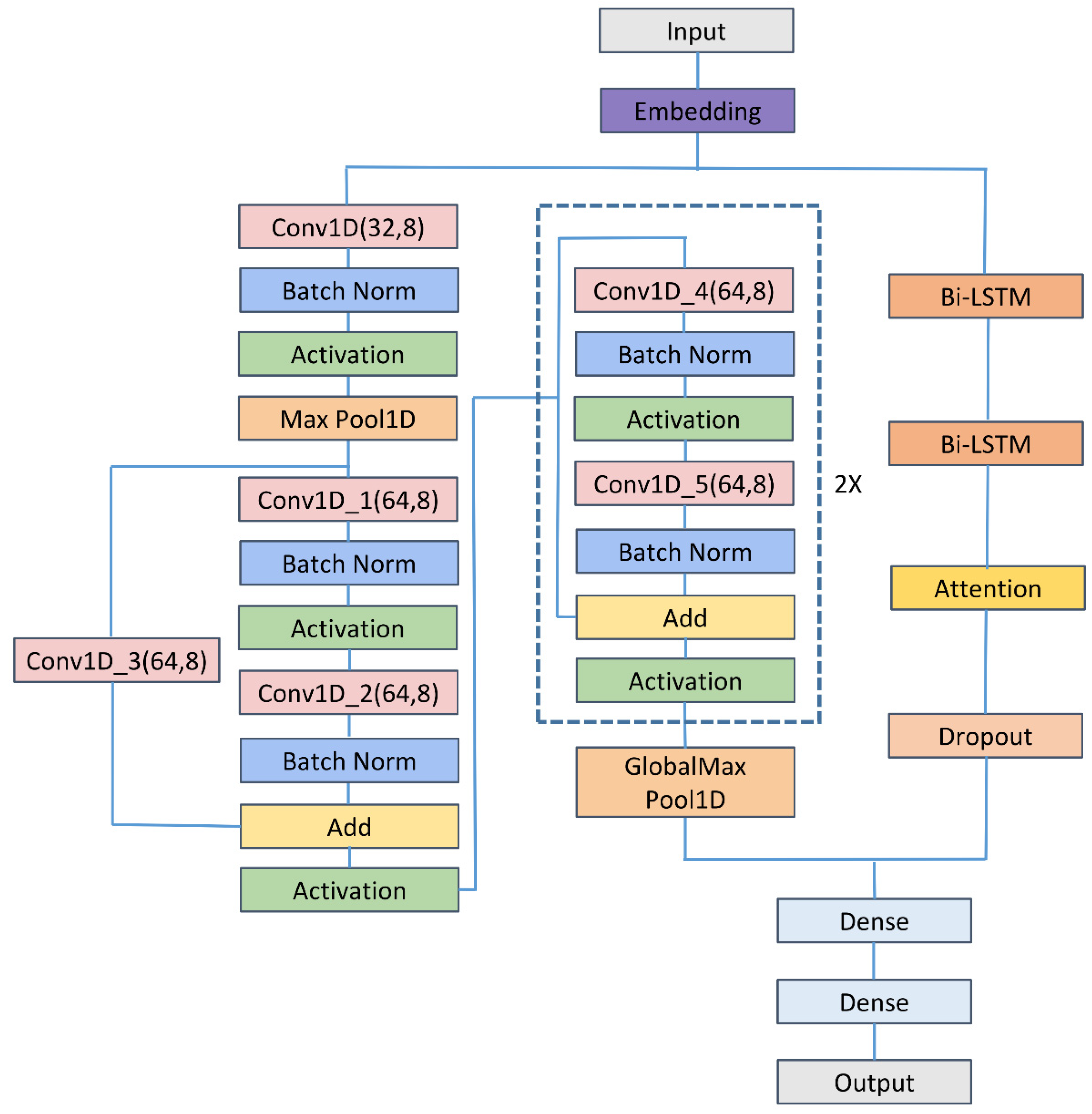
As shown in
Figure 1, the proposed method comprised mainly input, embedding, 1D CNN, residual neural network (ResNet), Bi-LSTM, attention, dropout, flattened, and fully connected layers. The input was DNA segments of 200 bp. Then, DNA segments were transformed into number sequences by
where N denoted the characters of the unknown nucleotide. The embedding of number sequences was entered into the convolution module and the LSTM module. The convolution module consisted mainly of the 1D CNN and ResNet [
81,
82,
83], while the LSTM module comprised mainly Bi-LSTM [
84,
85] and feed-forward attention [
86,
87]. The concatenation of outputs of the two modules was entered into the fully connected layer. Following the fully connected layer was the final layer, which contained one neuron representing the probabilities of belonging to enhancers. We set the threshold to 0.5, and thus more than 0.5 output indicated that the corresponding input was predicted to be positive and otherwise to be negative. The numbers of the parameters and the shape of output in each layer of the Enhancer-LSTMAtt were listed in
Table 1.
3.1. Embedding Layer
The embedding is generally the first layer of the deep neural network, whose role is to map the categorical (discrete) variable to continuous vectors (
https://towardsdatascience.com/neural-network-embeddings-explained-4d028e6f0526 (accessed on 3 March 2022)) [
88]. The traditional one-hot encoding suffered from two defaults. One was that it was not capable of distinguishing similarities between representations. Another was that the representation was sparse in the case of the large vocabulary. The embedding well solved two issues and thus was widely applied to the area of natural language processing. The embedding can be used alone, such as word2vec and Glove, or fused into the deep neural network as the first layer.
3.2. CNN
CNN is one of most popular neural network architectures used to construct deep neural network [
67,
89,
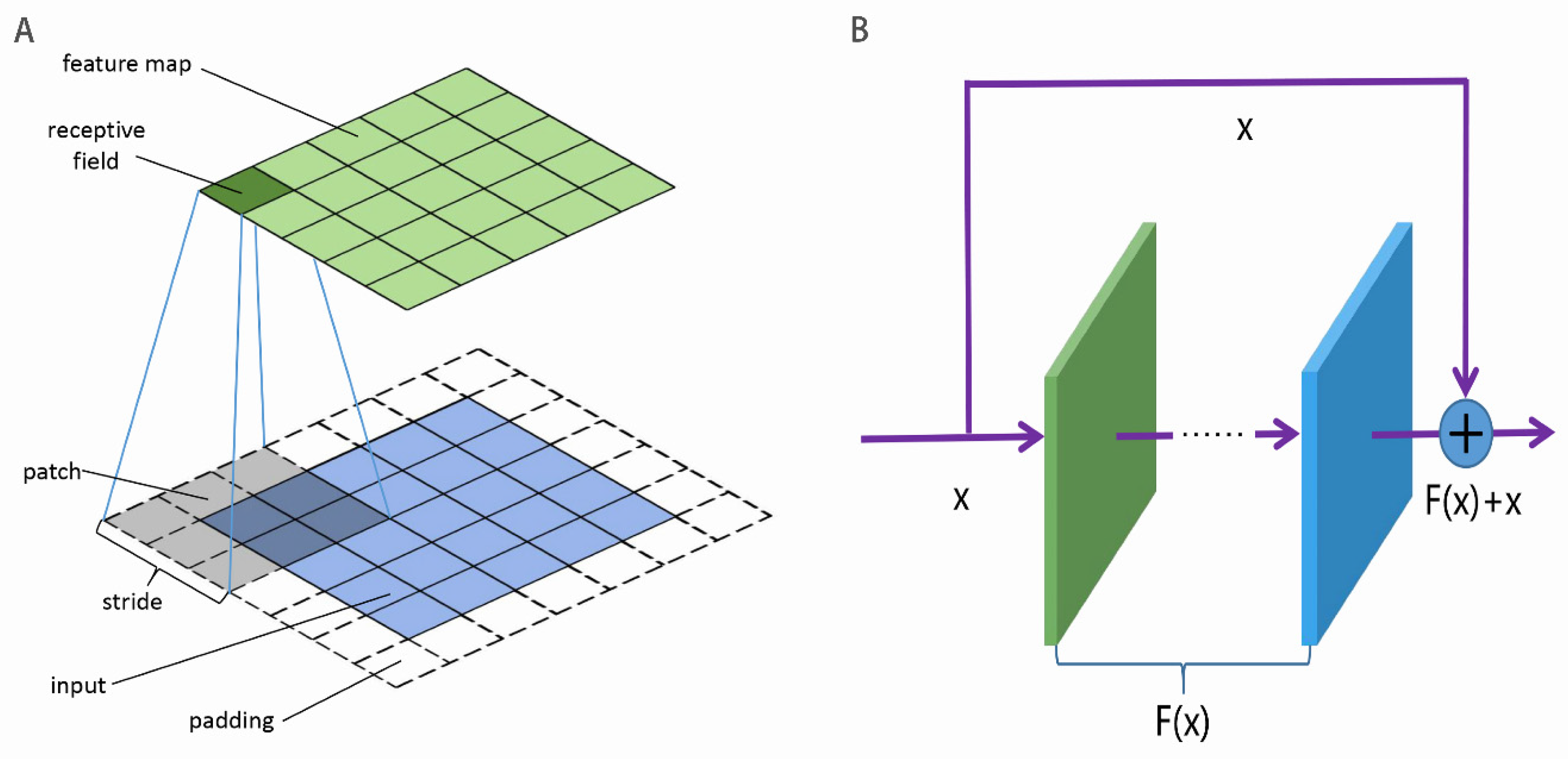
90]. The main characteristic of the CNN is to capture the local hidden structure by using convolutional kernels or filters. As shown in
Figure 2A, the input is divided into patches, which are convoluted into the feature map by the convolutional kernel. The patches are allowed to overlap, and the interval between adjacent patches is called the stride. All of the patches in the same input share the convolutional kernel which are learnable parameters. To keep the size of the input unchanged, the input is sometimes required to pad. To increase the non-linear ability of the CNN, the activation function is added to the feature map. The activation function includes ReLU, sigmoid, tanh, weakly ReLU, and ELU. The pooling in the CNN is a non-linear down-sampling, whose role is to reduce the dimensionality of representations and to speed up the calculation. In addition, the pooling is able to avoid or decrease the over-fitting issue.
3.3. ResNet
As the number of stacked layers in the deep neural network increased, three issues would occur: information loss, gradient vanishing or exploding, and network degradation. This resulted in the worse performance of the deep neural network [
89]. He el al. [
81] presented ResNet to address these issues. The basic architecture of ResNet [
81] was composed of residual mapping
and identity mapping x, as shown in
Figure 2B. The identify mapping ensured no loss of inputted information in spite of increasing layers. The residual mapping was viewed as the learnable residual function and might be conventional convolutions. The ResNet enabled the neural network to go deeper without network degradation. Li et al. [
81] used ResNet to construct a 152-layers deep network, which reduced the top 5 error rates of image recognition to 5.71% on the ImageNet.
3.4. Bi-LSTM
Long-short term memory (LSTM) [
90] is a type of recurrent neural network (RNN) [
91,
92]. The RNN is especially suitable to deal with time series questions due to its architecture: sharing weights at all of the time steps. The RNN was applied to a wide range of fields, including speech recognition [
93], continuous B-cell epitope prediction [
94], sentiment analysis [
95], and action recognition [
96]. The major default of the RNN was that it is prone to cause gradient vanishing or exploding for long sequence analysis. Therefore, the RNN was restricted to short sequences [
97,
98]. The LSTM [
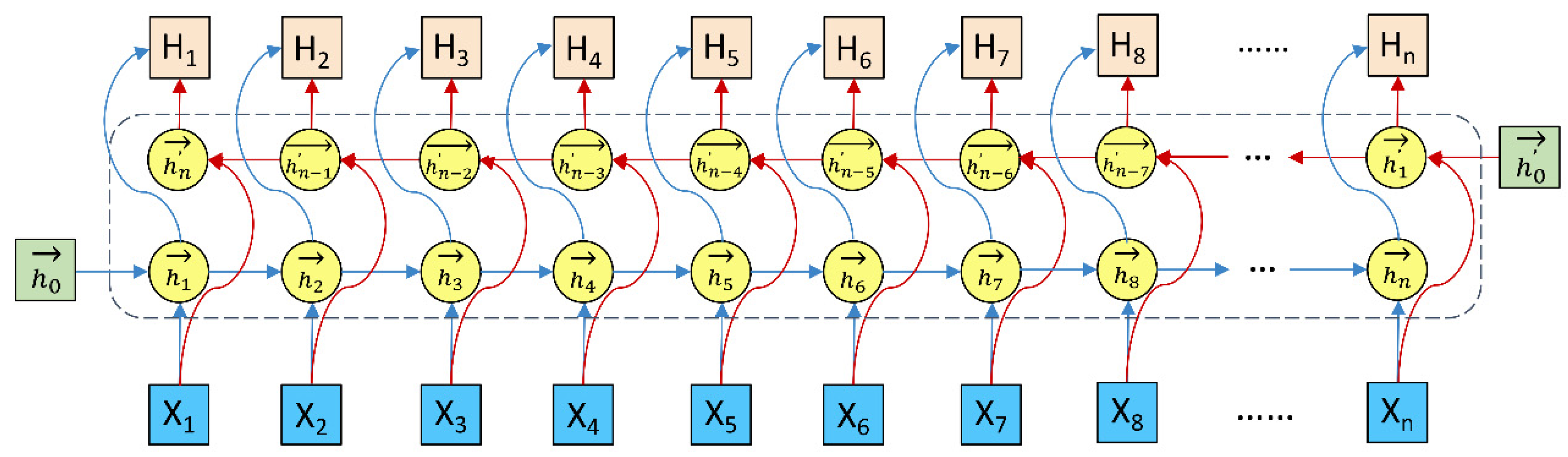
90] employed the gate mechanism to control conveying of information, including selective addition of new information or removal of information accumulated previously. The LSTM was able to capture the relationship of the words in the former with those in the back but was not able to characterize the relationship of the words in the back with those in the former. The Bi-LSTM [
84,
85] addressed the issue well. As shown in
Figure 3, the Bi-LSTM was made up of two LSTMs, one from forward to backward and another from backward to forward. The two LSTMs shared embedding of words but were independent of each other in terms of learnable parameters. The concatenation of hidden states in both LSTMs corresponded to the output of the Bi-LSTM.
3.5. Feed-Forward Attention
Attention mechanisms are increasingly becoming a hot topic in the field of deep learning. The attention mechanisms are a scheme of allocating weights, which is very similar to the scene where one assigns a different focus to different parts when watching an object. There are many attention schemes, including feed-forward attention [
99] and self-attention [
100], etc. The feed-forward attention is intended to make up for the deficiency of the LSTM in the long-term dependency. Assume that the hidden state at time step t in the LSTM was
. The context vector generated by the feed-forward attention was computed by
where
was the attention weight of the hidden state
.
was defined by
where
was the learnable parameter.
3.6. Dropout Layer
Dropout proposed by Hinton et al. [
101] is a concept to train deep neural network. In the process of training, a certain proportion of neurons are randomly dropped out, and all of the neurons are used as usual in the process of prediction [
102]. The dropout serves two-fold functions: speeding up training of the deep neural network and reducing over-fitting.
3.7. Flatten Layer and Fully Connected Layer
The flatten layer was intended to convert the shape of data so as to link conveniently the next layers. The flatten layers did not have any learnable parameters. The fully connected layer was identical to the hidden layer in the multilayer perceptron, and each neuron was connected to all of the neurons in the previous layer.
4. Cross Validation and Evaluation Metrics
To examine the predictive performance of the presented method, we used n-fold cross validation and independent test. In the n-fold cross-validation, the training dataset was divided into n parts of equal or approximately equal size, of which n-1 parts were used to train the model and the remaining part was used to test the model. This process was repeated n times. In the independent test, the training dataset was used to train the model, and the independent dataset was used to test the model.
This is a binary classification issue, so we used common metrics to evaluate the predictive performance, including sensitivity (SN), specificity (SP), accuracy (ACC), and Matthews’ correlation coefficient (MCC), which are defined as
where TP is the number of true positive samples, FN is the number of false negative samples, FP is the number of false positive samples, and TN is the number of true negative samples. SN, SP and ACC lie between 0 and 1. The MCC ranges from −1 to 1. More values of SN, SP, ACC and MCC indicated better performance.
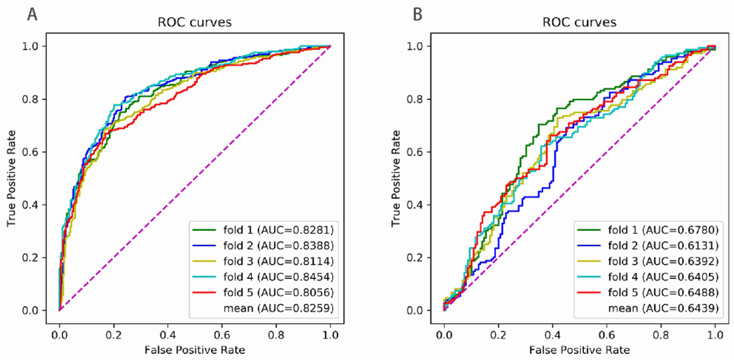
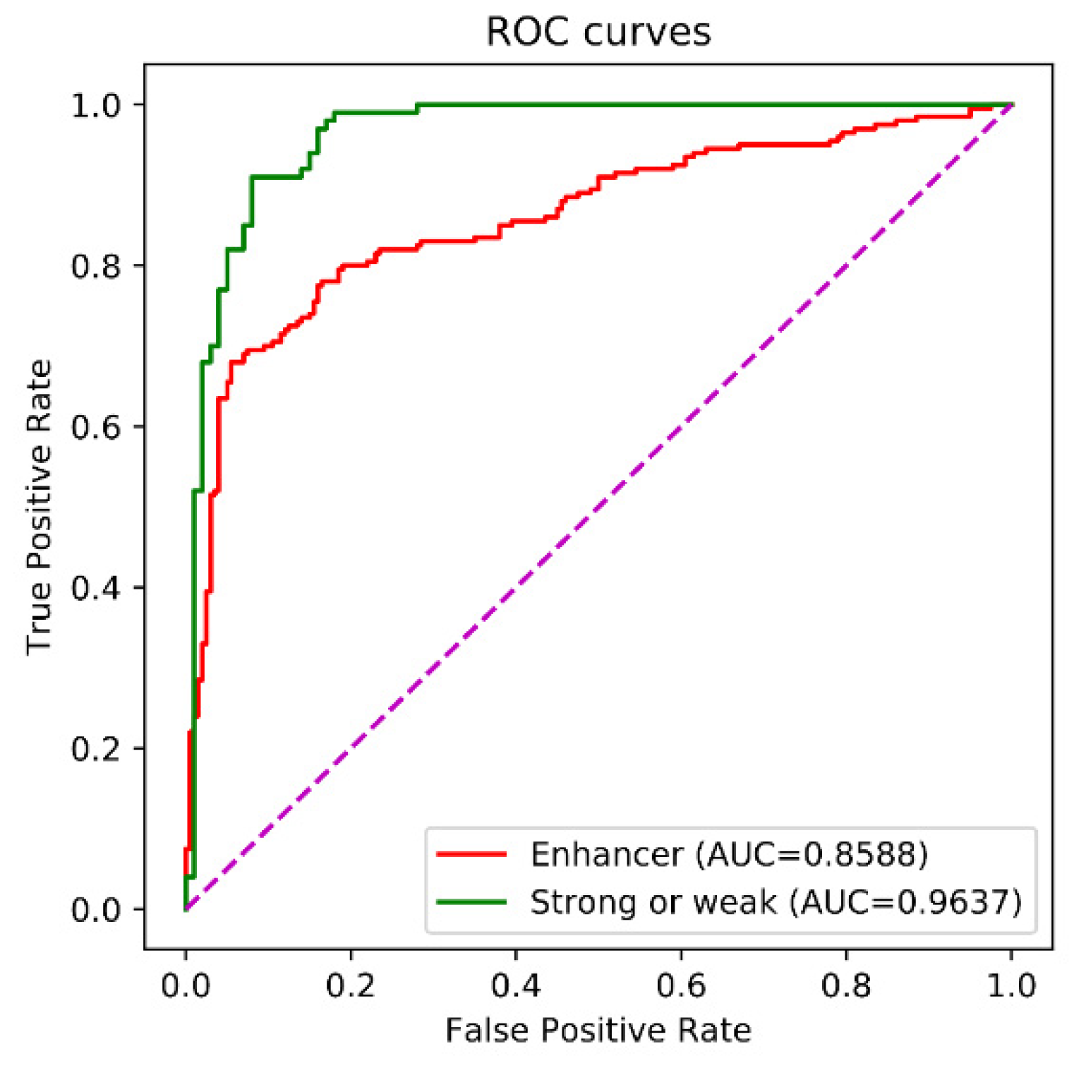
The receiver operating characteristic (ROC) curve is a commonly used way to evaluate the performance of binary classification methods. The ROC curve is drawn by plotting the true positive rate (TPR) against the false positive rate (FPR) under various thresholds. The TPR and the FPR are computed by
The area under the ROC curve (AUC) ranges from 0 to 1. If the AUC was equal to 1, the prediction was perfect. The AUC equaling 0.5 indicated a random prediction and the AUC equaling to 0 was an opposite prediction.
We used Python programming language along with the deep learning toolkit TensorFlow (version 2.0) to implement the Enhancer-LSTMAtt. We conducted 5-fold cross validation, 10-fold cross validation and independent test on the Microsoft Windows 10 operating system, which is installed on a notebook computer with 32G RAM and 6 CPUs, each with 2.60 GHz. Each epoch costs about 25 s in the training process, while prediction of each sample takes no more than 2 s by using the trained Enhancer-LSTMAtt. The codes along with the datasets are available at Github:
https://github.com/feng-123/Enhancer-LSTMAtt.


