
Fewer Dimensions, More Structures for Improved Discrete Models of Dynamics of Free versus Antigen-Bound Antibody


Abstract
:1. Introduction
2. Background
2.1. Related Work on MSMs of Structural Dynamics
2.2. Molecular System of Interest
2.2.1. Free Antibody and Antigen-Bound Antibody Structure Data
2.2.2. Prior MSM-Based Investigation
3. Methods
3.1. Shape-Based Coordinates/Features
- 1.
- The molecular centroid (ctd);
- 2.
- The closest atom to ctd (cst);
- 3.
- The furthest atom from ctd (fct);
- 4.
- The furthest atom to fct (ftf).
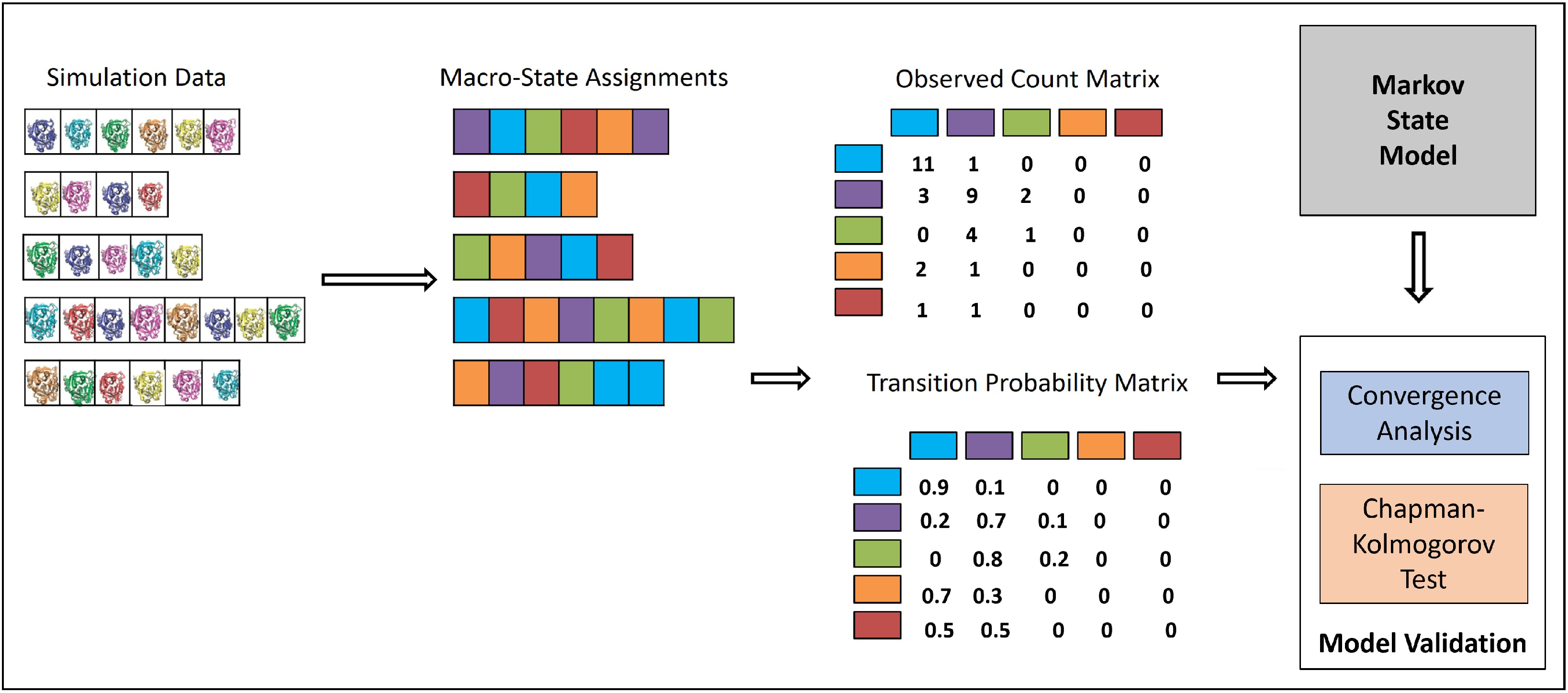
3.2. Integrating MD Trajectories in an MSM
Statistical Tests of MSM Quality
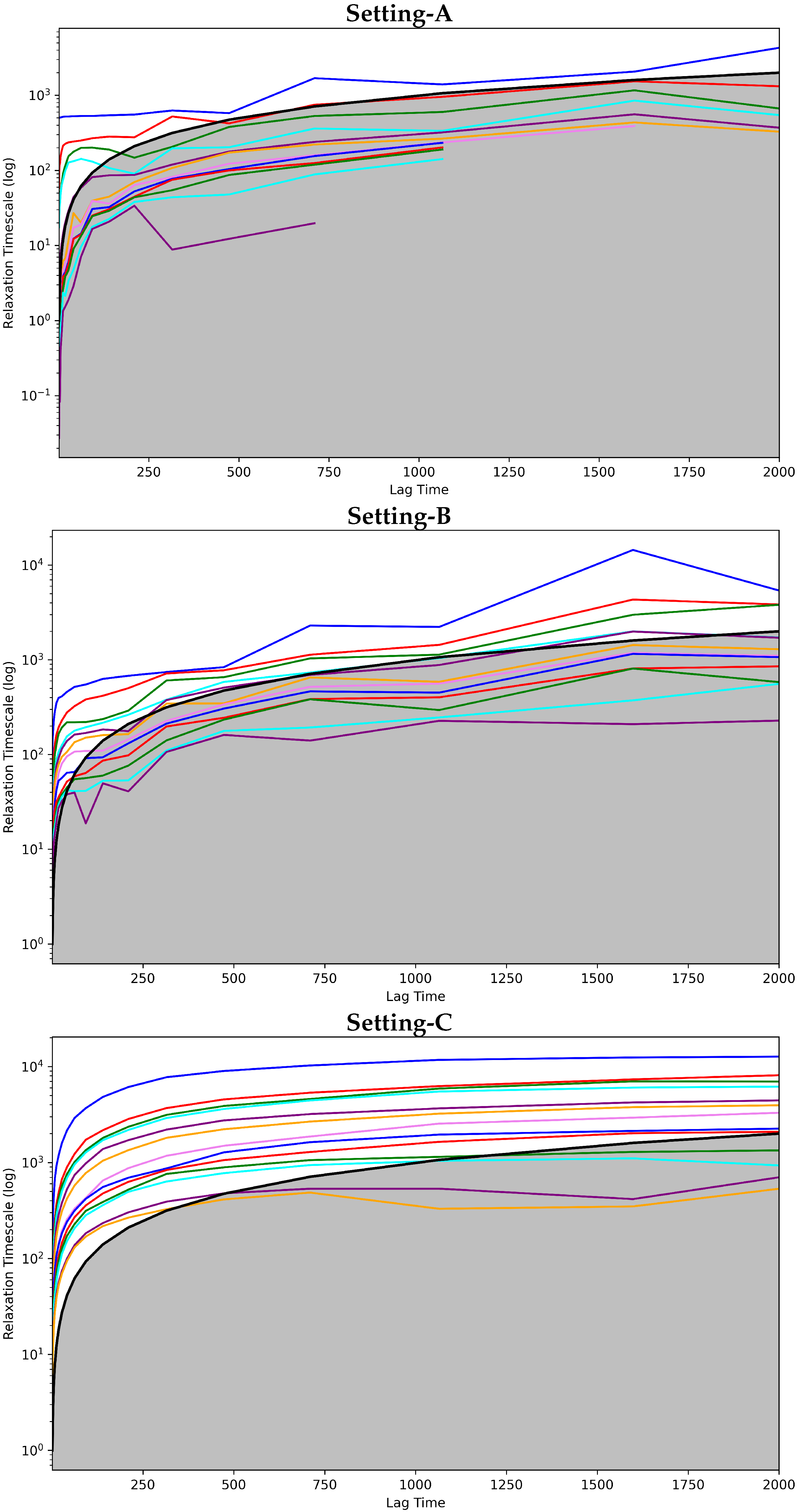
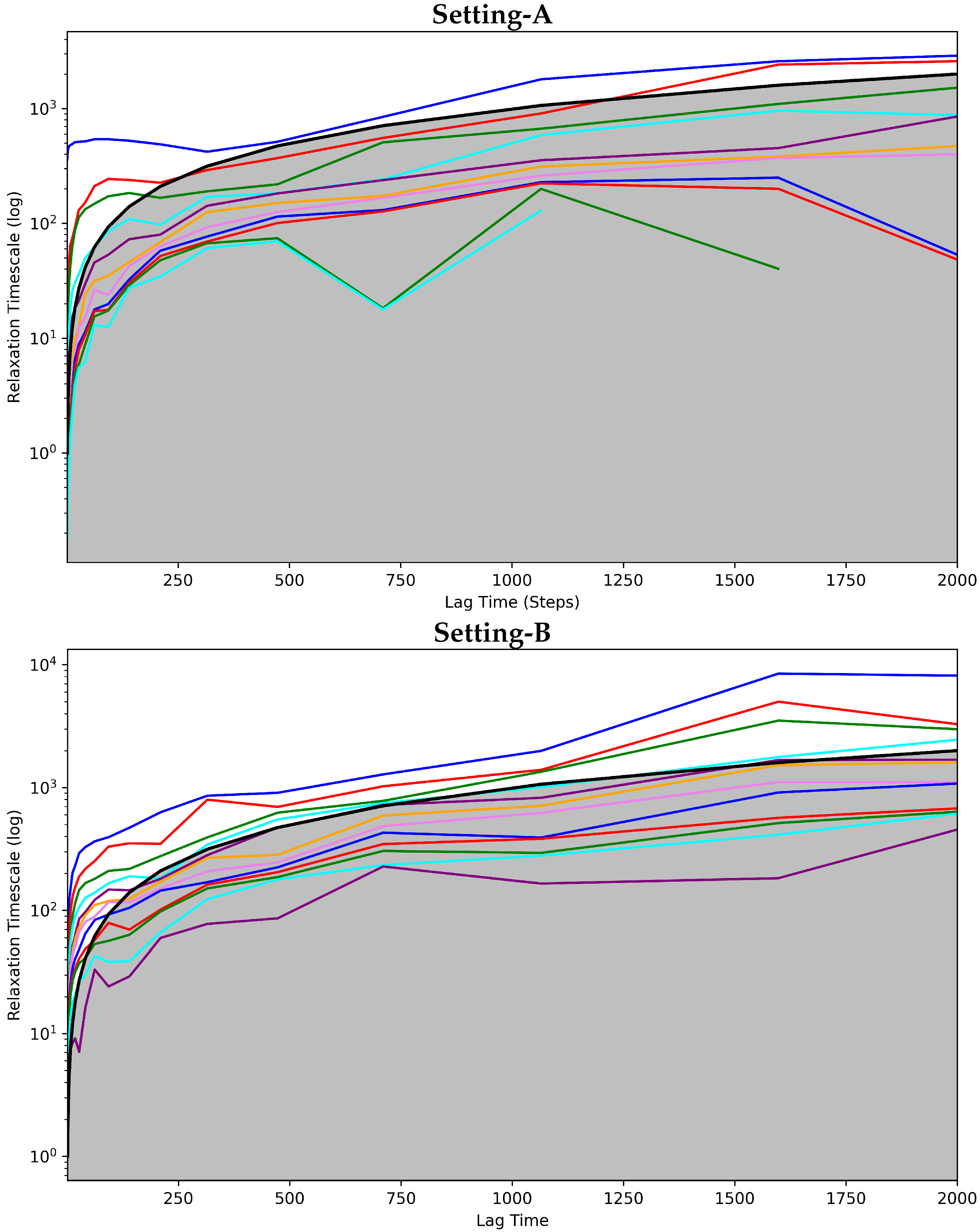
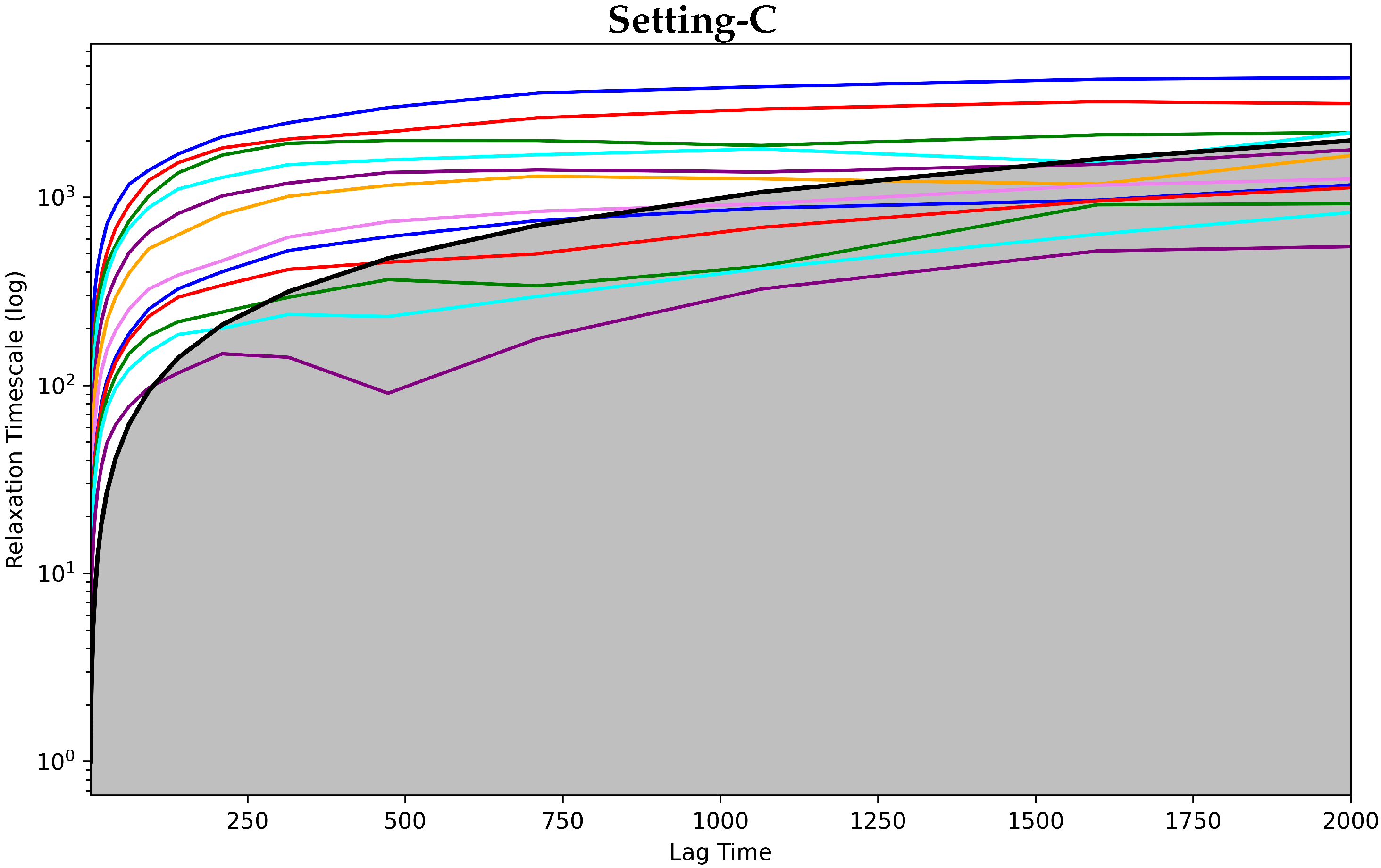
Convergence Analysis
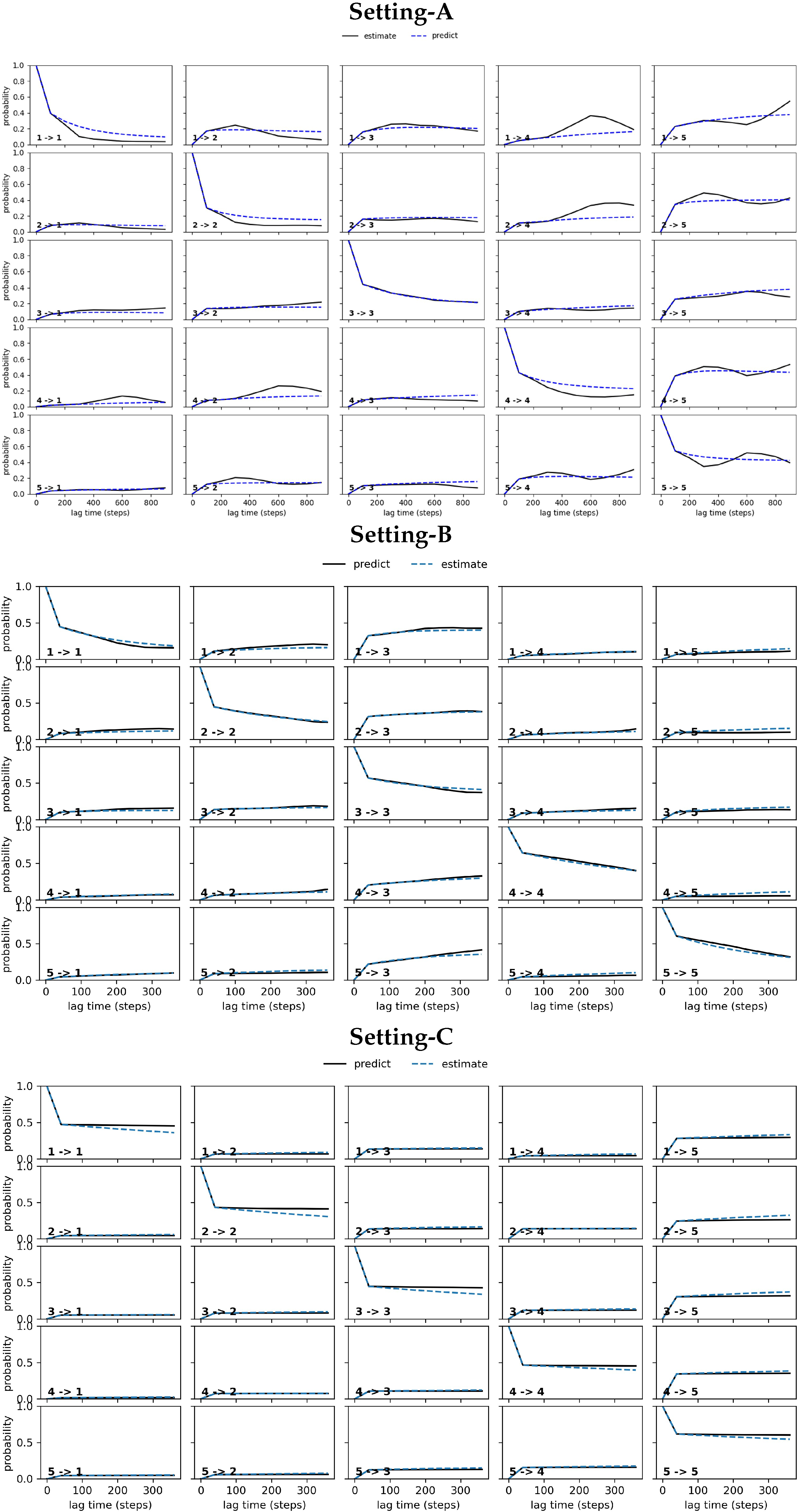
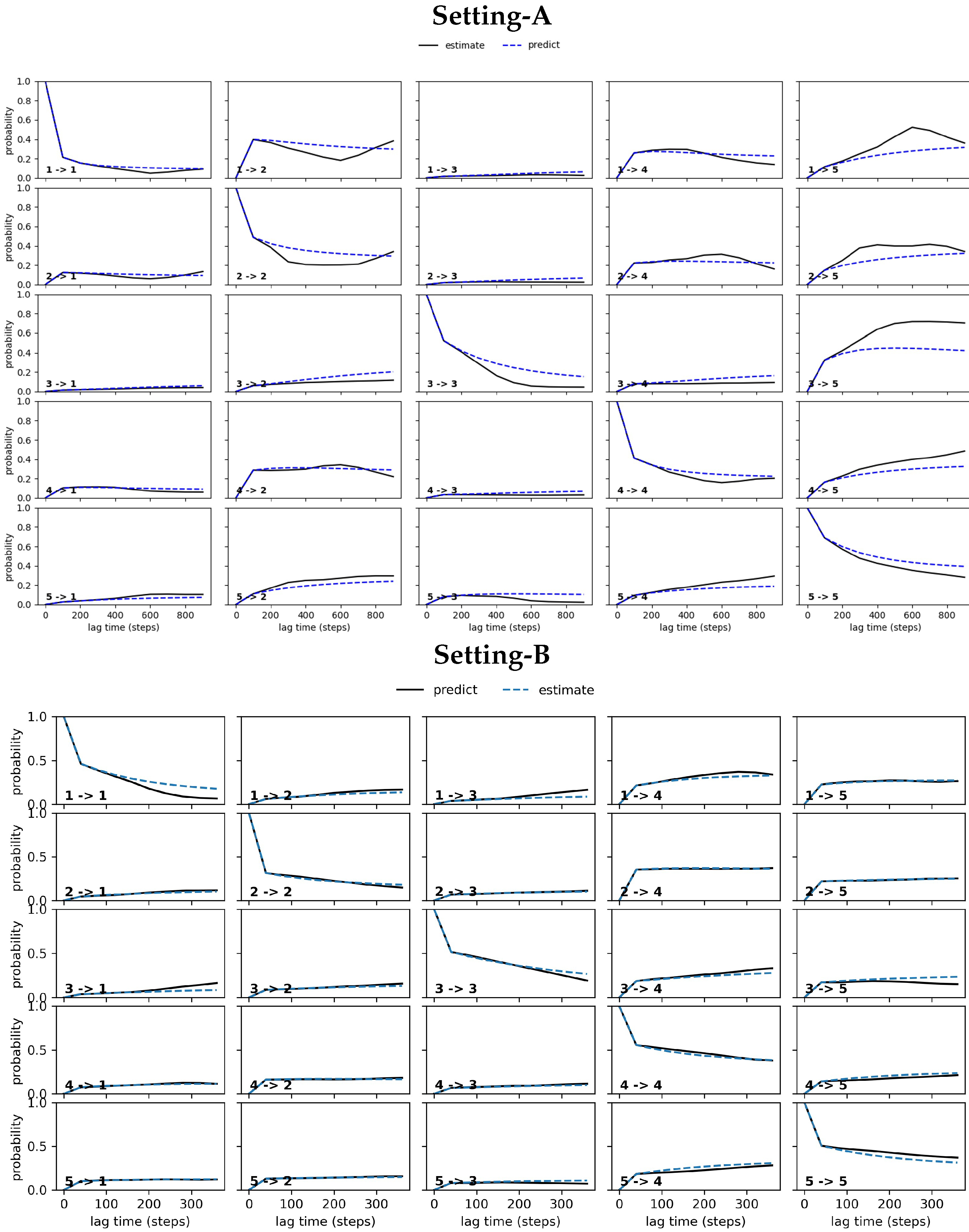
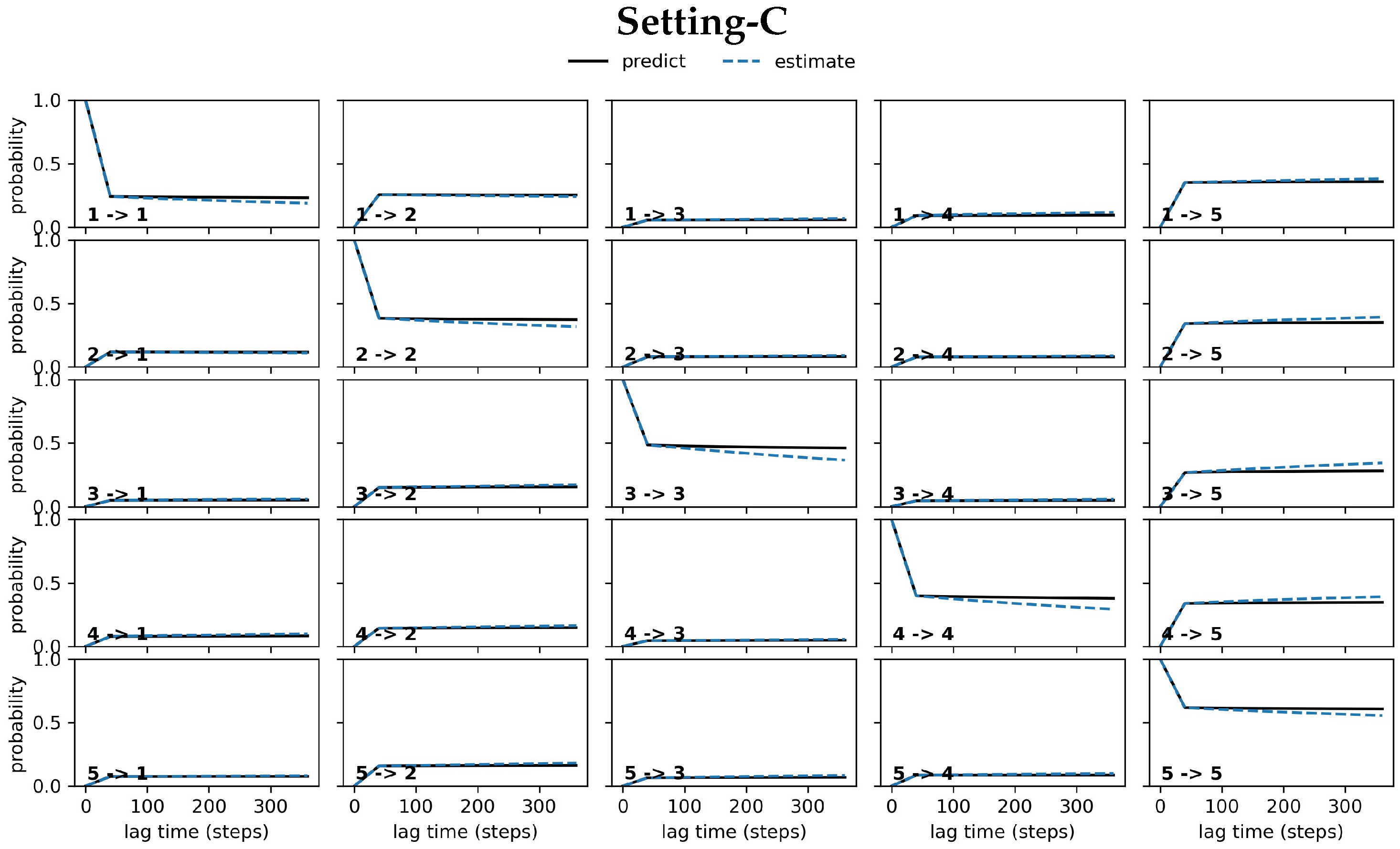
CK Test
4. Results
4.1. Evaluation Setup
4.2. Comparison of Models of Free Antibody Dynamics
4.2.1. Free Antibody MSM Evaluation via the Convergence Analysis
4.2.2. Free Antibody MSM Evaluation via the CK Test
4.3. Comparison of Models of Antigen-Bound Antibody Dynamics
4.3.1. Antigen-Bound Antibody MSM Evaluation via the Convergence Analysis
4.3.2. Antigen-Bound Antibody MSM Evaluation via the CK Test
4.3.3. Run-Time Comparison
4.4. Comparison of Free vs. Antigen-Bound Antibody Dynamics
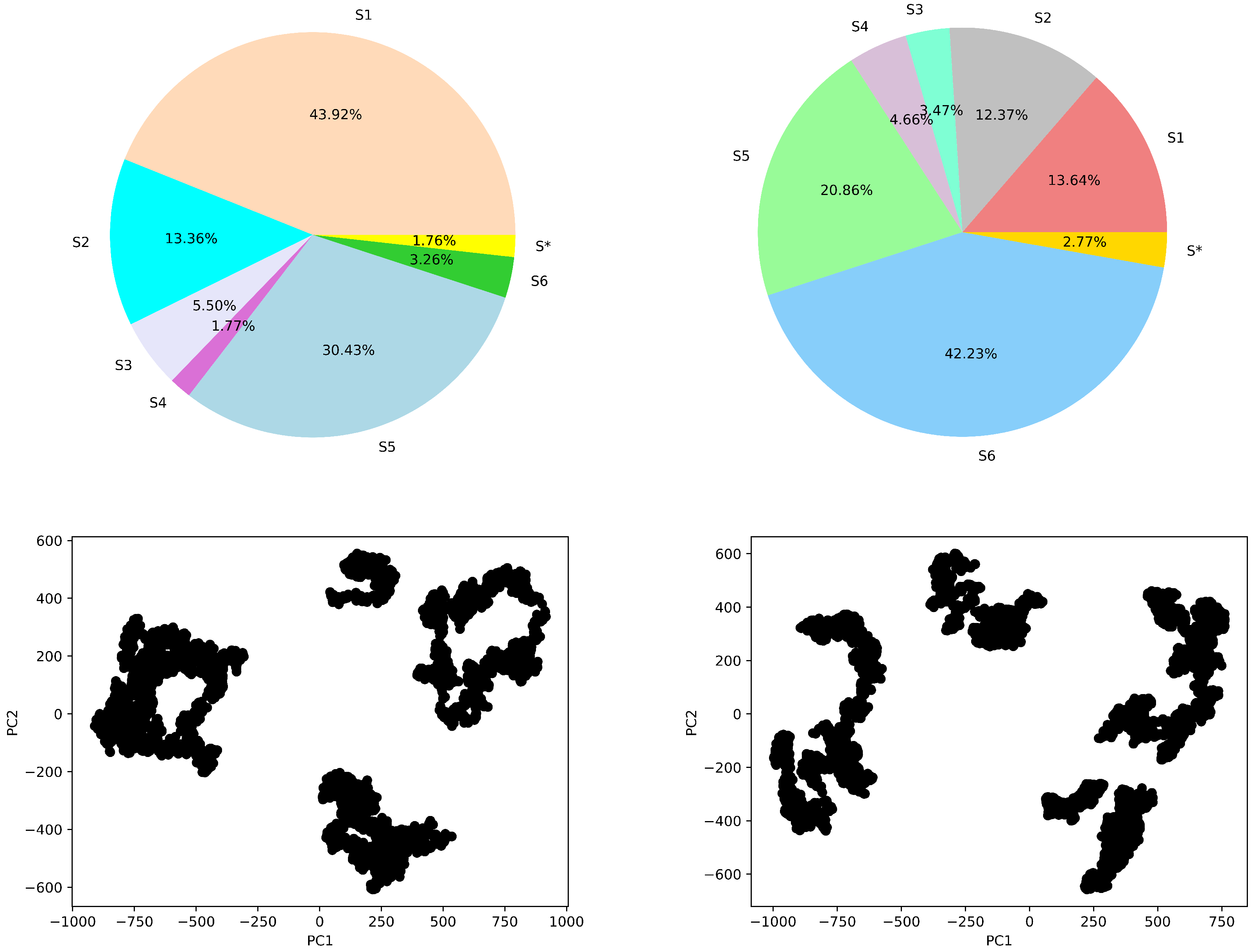
4.4.1. Macro-State Analysis: Comparison of Stationary State Distributions
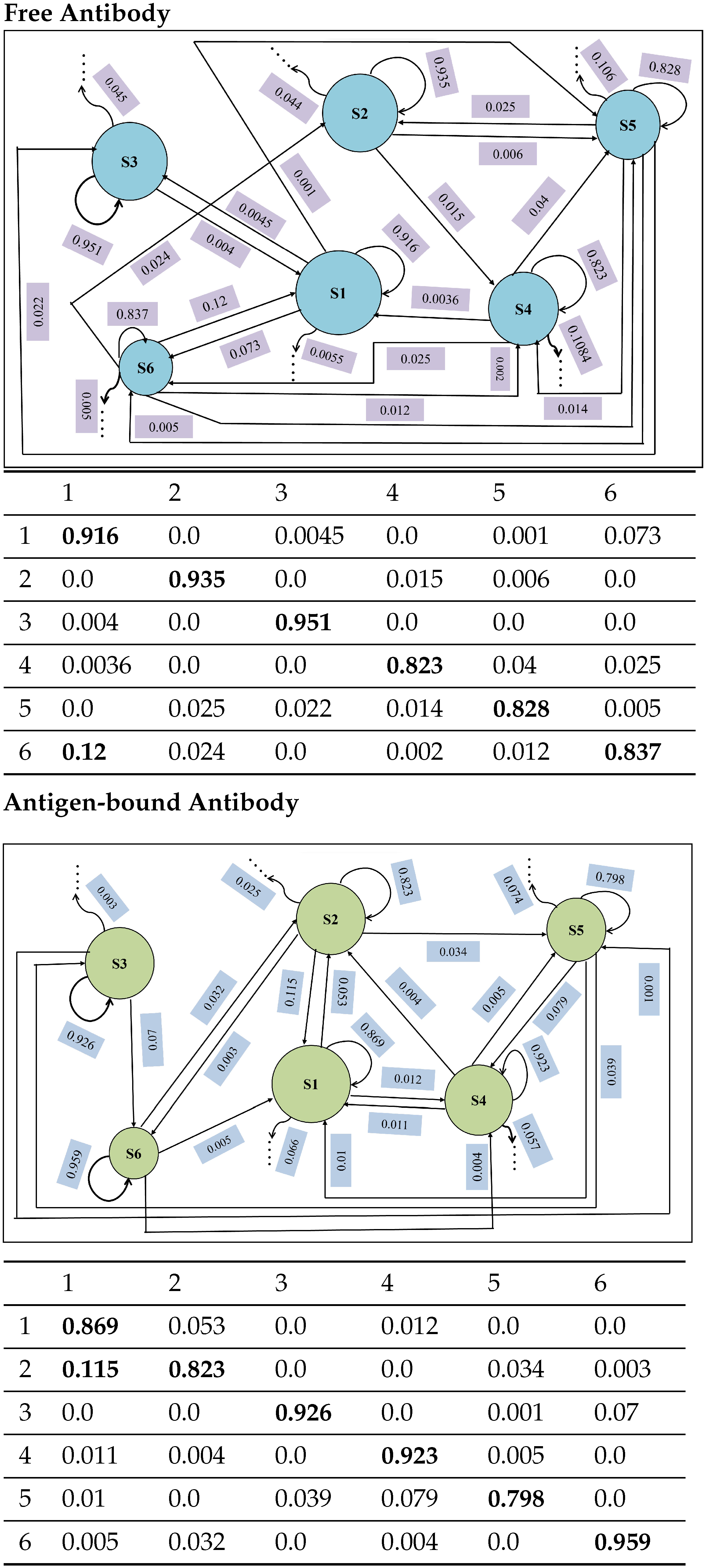
4.4.2. State-to-State Dynamics: Comparison of State Transitions
5. Conclusions
Supplementary Materials
Author Contributions
Funding
Institutional Review Board Statement
Informed Consent Statement
Data Availability Statement
Acknowledgments
Conflicts of Interest
Abbreviations
| CA Atom | Carbon Alpha Atom |
| CK Test | Chapman–Kolmogorov Test |
| GBMV | Generalized Born method using Molecular Volume |
| MD | Molecular Dynamics |
| MSM | Markov State Model |
| PCA | Principal Component Analysis |
| TICA | Time-lagged Independent Component Analysis |
| USR | Ultrafast Shape Recognition |
References
- Jumper, J.; Evans, R.; Pritzel, A.; Green, T.; Figurnov, M.; Ronneberger, O.; Tunyasuvunakool, K.; Bates, R.; Žídekdek, A.; Potapenko, A.; et al. Highly accurate protein structure prediction with AlphaFold. Nature 2021, 596, 583–589. [Google Scholar] [PubMed]
- Tunyasuvunakool, K.; Adler, J.; Wu, Z.; Green, T.; Zielinski, M.; Žídekdek, A.; Bridgl, A.; Cowie, A.; Meyer, C.; Laydon, A.; et al. Highly accurate protein structure prediction for the human proteome. Nature 2021, 595, 590–596. [Google Scholar]
- Akdel, M.; Pires, D.E.V.; Porta, P.; Pardo, E.; Jänes, J.A. A structural biology community assessment of AlphaFold 2 applications. bioRxiv 2021. [Google Scholar] [CrossRef]
- Maximova, T.; Moffatt, R.; Ma, B.; Nussinov, R.; Shehu, A. Principles and Overview of Sampling Methods for Modeling Macromolecular Structure and Dynamics. PLoS Comp. Biol. 2016, 12, e1004619. [Google Scholar]
- Pande, V.J.; Beauchamp, K.; Bowman, G.R. Everything you wanted to know about Markov State Models but were afraid to ask. Methods 2010, 52, 99–105. [Google Scholar]
- Chodera, J.D.; Noé, F. Markov state models of biomolecular conformational dynamics. Curr. Opin. Struct. Biol. 2014, 25, 135–144. [Google Scholar]
- Taylor, B.C.; Lee, C.T.; Amaro, R.E. Structural basis for ligand modulation of the CCR2 conformational landscape. Proc. Natl. Acad. Sci. USA 2019, 116, 8131–8136. [Google Scholar]
- Plattner, N.; Doerr, S.; De Fabritiis, G.; Noé, F. Complete protein–protein association kinetics in atomic detail revealed by molecular dynamics simulations and Markov modelling. Nat. Chem. 2017, 9, 1005. [Google Scholar]
- Plattner, N.; Noé, F. Protein conformational plasticity and complex ligand-binding kinetics explored by atomistic simulations and Markov models. Nat. Commun. 2015, 6, 7653. [Google Scholar]
- Malmstrom, R.D.; Lee, C.T.; Van Wart, A.T.; Amaro, R.E. Application of molecular-dynamics based markov state models to functional proteins. J. Chem. Theory Comput. 2014, 10, 2648–2657. [Google Scholar]
- Schwantes, C.R.; Pande, V.S. Improvements in Markov state model construction reveal many non-native interactions in the folding of NTL9. J. Chem. Theory Comput. 2013, 9, 2000–2009. [Google Scholar] [PubMed] [Green Version]
- Kabir, K.L.; Akhter, N.; Shehu, A. From molecular energy landscapes to equilibrium dynamics via landscape analysis and markov state models. J. Bioinf. Comput. Biol. 2019, 17, 1940014. [Google Scholar]
- Kabir, K.L.; Akhter, N.; Shehu, A. Connecting molecular energy landscape analysis with markov model-based analysis of equilibrium structural dynamics. In Proceedings of the International Conference on Bioinformatics and Computational Biology (BICOB), Honolulu, HI, USA, 18–20 March 2019; Volume 60, pp. 181–189. [Google Scholar]
- Kabir, K.L.; Hassan, L.; Rajabi, Z.; Akhter, N.; Shehu, A. Graph-based community detection for decoy selection in template-free protein structure prediction. Molecules 2019, 24, 854. [Google Scholar]
- Cazals, F.; Dreyfus, T. The structural bioinformatics library: Modeling in biomolecular science and beyond. Bioinformatics 2017, 33, 997–1004. [Google Scholar] [PubMed] [Green Version]
- Kabir, K.L.; Nussinov, R.; Ma, B.; Shehu, A. Antigen Binding Reshapes Antibody Energy Landscape and Conformation Dynamics. In Proceedings of the 2021 IEEE International Conference on Bioinformatics and Biomedicine (BIBM), Houston, TX, USA, 9–12 December 2021; pp. 2519–2526. [Google Scholar]
- Ballester, P.J.; Richards, W.G. Ultrafast shape recognition to search compound databases for similar molecular shapes. J. Comput. Chem. 2007, 28, 1711–1723. [Google Scholar]
- Zaman, A.B.; Kamranfar, P.; Domeniconi, C.; Shehu, A. Reducing ensembles of protein tertiary structures generated de novo via clustering. Molecules 2020, 25, 2228. [Google Scholar]
- Shehu, A.; Olson, B. Guiding the Search for Native-like Protein Conformations with an Ab-initio Tree-based Exploration. Intl. J. Robot. Res. 2010, 29, 1106–1127. [Google Scholar]
- Zaman, A.B.; De Jong, K.A.; Shehu, A. Guiding Protein Conformation Sampling with Conformation Space Maps. In Proceedings of the International Conference on Bioinformatics and Computational Biology (BICOB), Online, 21–23 March 2022; Volume 83, pp. 20–30. [Google Scholar]
- Molloy, K.; Shehu, A. Elucidating the Ensemble of Functionally-relevant Transitions in Protein Systems with a Robotics-inspired Method. BMC Struct. Biol. 2013, 13, S8. [Google Scholar]
- Zwanzig, R. From classical dynamics to continuous time random walks. J. Stat. Phys. 1983, 30, 255–262. [Google Scholar]
- Husic, B.E.; Pande, V.J. Markov State Models: From an Art to a Science. J. Am. Chem. Soc. 2018, 140, 2386–2396. [Google Scholar]
- Harrigan, M.P.; Sultan, M.M.; Hernndez, C.X.; Husic, B.E.; Eastman, P.; Schwantes, C.R.; Beauchamp, K.A.; McGibbon, R.T.; Pande, V.S. MSMBuilder: Statistical Models for Biomolecular Dynamics. Biophys. J. 2017, 112, 10–15. [Google Scholar] [CrossRef] [PubMed] [Green Version]
- Senne, M.; Trendelkamp-Schroer, B.; Mey, A.S.; Schutte, C.; Noé, F. EMMA: A Software Package for Markov Model Building and Analysis. J. Chem. Theory Comput. 2012, 8, 2223–2238. [Google Scholar] [CrossRef] [PubMed]
- Scherer, M.K.; Trendelkamp-Schroer, B.; Paul, F.; Pérez-Hernández, G.; Hoffmann, M.; Plattner, N.; Wehmeyer, C.; Prinz, J.; Noé, F. PyEMMA 2: A Software Package for Estimation, Validation, and Analysis of Markov Models. J. Chem. Theory Comput. 2015, 11, 5525–5542. [Google Scholar] [CrossRef]
- Bowman, G.R.; Beauchamp, K.A.; Boxer, G.; Pande, V.S. Progress and challenges in the automated construction of Markov state models for full protein systems. J. Chem. Phys. 2009, 131, 124101. [Google Scholar] [CrossRef] [Green Version]
- Ratcliffe, M.J.H. (Ed.) Encyclopedia of Immunobiology; Elsevier: Amsterdam, The Netherlands, 2016; Volume 7, p. 3126. [Google Scholar]
- Keskin, O. Binding induced conformational changes of proteins correlate with their intrinsic fluctuations: A case study of antibodies. BMC Struct. Biol. 2007, 7, 31. [Google Scholar] [CrossRef] [PubMed]
- Thielges, M.C.; Zimmermann, J.; Yu, W.; Oda, M.; Romesberg, F.E. Exploring the energy landscape of antibody− antigen complexes: Protein dynamics, flexibility, and molecular recognition. Biochemistry 2008, 47, 7237–7247. [Google Scholar] [CrossRef]
- Li, T.; Tracka, M.B.; Uddin, S.; Casas-Finet, J.; Jacobs, D.J.; Livesay, D.R. Redistribution of flexibility in stabilizing antibody fragment mutants follows Le Chatelier’s principle. PLoS ONE 2014, 9, e92870. [Google Scholar]
- Zhao, J.; Nussinov, R.; Ma, B. Antigen binding allosterically promotes Fc receptor recognition. MAbs 2019, 11, 58–74. [Google Scholar] [CrossRef]
- Chen, Y.; Wei, G.; Zhao, J.; Nussinov, R.; Ma, B. Computational Investigation of Gantenerumab and Crenezumab Recognition of Abeta Fibrils in Alzheimer’s Disease Brain Tissue. ACS Chem. Neurosci. 2020, 11, 3233–3244. [Google Scholar] [CrossRef]
- Sela-Culang, I.; Kunik, V.; Ofran, Y. The structural basis of antibody–antigen recognition. Front. Immunol. 2013, 4, 302. [Google Scholar] [CrossRef] [Green Version]
- Pritsch, O.; Hudry-Clergeon, G.; Buckle, M.; Petillot, Y.; Bouvet, J.P.; Gagnon, J.; Dighiero, G. Can immunoglobulin C(H)1 constant region domain modulate antigen binding affinity of antibodies? J. Clin. Investig. 1996, 98, 2235. [Google Scholar] [CrossRef] [PubMed]
- Adachi, M.; Kurihara, Y.; Nojima, H.; Takeda-Shitaka, M.; Kamiya, K.; Umeyama, H. Interaction between the antigen and antibody is controlled by the constant domains: Normal mode dynamics of the HEL–HyHEL-10 complex. Protein Sci. 2003, 12, 2125–2131. [Google Scholar] [CrossRef] [PubMed]
- Dam, T.K.; Torres, M.; Brewer, C.F.; Casadevall, A. Isothermal titration calorimetry reveals differential binding thermodynamics of variable region-identical antibodies differing in constant region for a univalent ligand. J. Biol. Chem. 2008, 283, 31366–31370. [Google Scholar] [CrossRef] [PubMed] [Green Version]
- Tudor, D.; Yu, H.; Maupetit, J.; Drillet, A.S.; Bouceba, T.; Schwartz-Cornil, I.; Lopalco, L.; Tuffery, P.; Bomsel, M. Isotype modulates epitope specificity, affinity, and antiviral activities of anti–HIV-1 human broadly neutralizing 2F5 antibody. Proc. Natl. Acad. Sci. USA 2012, 109, 12680–12685. [Google Scholar] [CrossRef] [PubMed] [Green Version]
- Li, T.; Tracka, M.B.; Uddin, S.; Casas-Finet, J.; Jacobs, D.J.; Livesay, D.R. Rigidity Emerges during Antibody Evolution in Three Distinct Antibody Systems: Evidence from QSFR Analysis of Fab Fragments. PLoS Comput. Biol. 2015, 11, e1004327. [Google Scholar] [CrossRef] [Green Version]
- Janda, A.; Bowen, A.; Greenspan, N.S.; Casadevall, A. Ig Constant Region Effects on Variable Region Structure and Function. Front. Microbiol. 2016, 7, 22. [Google Scholar] [CrossRef] [Green Version]
- Janda, A.; Casadevall, A. Circular Dichroism reveals evidence of coupling between immunoglobulin constant and variable region secondary structure. Mol. Immunol. 2010, 47, 1421–1425. [Google Scholar] [CrossRef] [Green Version]
- Correa, A.; Trajtenberg, F.; Obal, G.; Pritsch, O.; Dighiero, G.; Oppezzo, P.; Buschiazzo, A. Structure of a human IgA1 Fab fragment at 1.55 resolution: Potential effect of the constant domains on antigen-affinity modulation. Acta Crystallogr. D Biol. Crystallogr. 2013, 69, 388–397. [Google Scholar] [CrossRef] [Green Version]
- Janda, A.; Eryilmaz, E.; Nakouzi, A.; Cowburn, D.; Casadevall, A. Variable region identical immunoglobulins differing in isotype express different paratopes. J. Biol. Chem. 2012, 287, 35409–35417. [Google Scholar] [CrossRef] [Green Version]
- Cooper, L.J.; Shikhman, A.R.; Glass, D.D.; Kangisser, D.; Cunningham, M.W.; Greenspan, N.S. Role of heavy chain constant domains in antibody–antigen interaction. Apparent specificity differences among streptococcal IgG antibodies expressing identical variable domains. J. Immunol. 1993, 150, 2231–2242. [Google Scholar]
- Torosantucci, A.; Chiani, P.; Bromuro, C.; De Bernardis, F.; Palma, A.S.; Liu, Y.; Mignogna, G.; Maras, B.; Colone, M.; Stringaro, A.; et al. Protection by anti-beta-glucan antibodies is associated with restricted beta-1,3 glucan binding specificity and inhibition of fungal growth and adherence. PLoS ONE 2009, 4, e5392. [Google Scholar] [CrossRef] [PubMed] [Green Version]
- Tomaras, G.D.; Ferrari, G.; Shen, X.; Alam, S.M.; Liao, H.X.; Pollara, J.; Bonsignori, M.; Moody, M.A.; Fong, Y.; Chen, X.; et al. Vaccine-induced plasma IgA specific for the C1 region of the HIV-1 envelope blocks binding and effector function of IgG. Proc. Natl. Acad. Sci. USA 2013, 110, 9019–9024. [Google Scholar] [CrossRef] [PubMed] [Green Version]
- Kato, K.; Matsunaga, C.; Odaka, A.; Yamato, S.; Takaha, W.; Shimada, I.; Arata, Y. Carbon-13 NMR study of switch variant anti-dansyl antibodies: Antigen binding and domain-domain interactions. Biochemistry 1991, 30, 6604–6610. [Google Scholar] [CrossRef] [PubMed]
- Torres, M.; May, R.; Scharff, M.D.; Casadevall, A. Variable-region-identical antibodies differing in isotype demonstrate differences in fine specificity and idiotype. J. Immunol. 2005, 174, 2132–2142. [Google Scholar] [CrossRef] [Green Version]
- Su, C.T.; Lua, W.; Ling, W.; Ga, S.K. Allosteric Effects between the Antibody Constant and Variable Regions: A Study of IgA Fc Mutations on Antigen Binding. Antibodies 2018, 7, 20. [Google Scholar] [CrossRef] [Green Version]
- Wang, W.; Chen, Q. Antigen improves binding of IgGs to FcγRs in SPR analysis. Anal. Biochem. 2022, 640, 114411. [Google Scholar] [CrossRef]
- Kalé, L.; Skeel, R.; Bhandarkar, M.; Brunner, R.; Gursoy, A.; Krawetz, N.; Phillips, J.; Shinozaki, A.; Varadarajan, K.; Schulten, K. NAMD2: Greater Scalability for Parallel Molecular Dynamics. J. Comput. Phys. 1999, 151, 283–312. [Google Scholar] [CrossRef]
- Huang, J.; MacKerell, A.D., Jr. CHARMM36 all-atom additive protein force field: Validation based on comparison to NMR data. J. Comput. Chem. 2013, 34, 2135–2145. [Google Scholar] [CrossRef] [Green Version]
- Steinbach, M.; Ertöz, L.; Kumar, V. The challenges of clustering high dimensional data. In New Directions in Statistical Physics; Springer: Berlin/Heidelberg, Germany, 2004; pp. 273–309. [Google Scholar]
- Akhter, N.; Shehu, A. From Extraction of Local Structures of Protein Energy Landscapes to Improved Decoy Selection in Template-free Protein Structure Prediction. Molecules 2018, 23, 216. [Google Scholar] [CrossRef] [Green Version]
- Akhter, N.; Qiao, W.; Shehu, A. An Energy Landscape Treatment of Decoy Selection in Template-free Protein Structure Prediction. Computation 2018, 6, 39. [Google Scholar] [CrossRef] [Green Version]
- Akhter, N.; Chennupati, G.; Kabir, K.L.; Djidjev, H.; Shehu, A. Unsupervised and supervised learning over the energy landscape for protein decoy selection. Biomolecules 2019, 9, 607. [Google Scholar] [CrossRef] [PubMed] [Green Version]
- Akhter, N.; Chennupati, G.; Djidjev, H.; Shehu, A. Decoy selection for protein structure prediction via extreme gradient boosting and ranking. BMC Bioinform. 2020, 21, 1–21. [Google Scholar] [CrossRef] [PubMed]
- Noé, F.; Nuske, F. A variational approach to modeling slow processes in stochastic dynamical systems. Multiscale Model. Simul. 2013, 11, 635–655. [Google Scholar] [CrossRef] [Green Version]
- Prinz, J.H.; Wu, H.; Sarich, M.; Keller, B.; Senne, M.; Held, M.; Chodera, J.D.; Schütte, C.; Noé, F. Markov models of molecular kinetics: Generation and validation. J. Chem. Phys. 2011, 134, 174105. [Google Scholar] [CrossRef] [PubMed]


| ID | Setting-A | Setting-B | Setting-C |
|---|---|---|---|
| Free Antibody | 1 h 41 m | 1 h 17 m | 26 m |
| Antigen-bound Antibody | 2 h 5 m | 1 h 44 m | 29 m |
Publisher’s Note: MDPI stays neutral with regard to jurisdictional claims in published maps and institutional affiliations. |
© 2022 by the authors. Licensee MDPI, Basel, Switzerland. This article is an open access article distributed under the terms and conditions of the Creative Commons Attribution (CC BY) license (https://creativecommons.org/licenses/by/4.0/).
Share and Cite
Kabir, K.L.; Ma, B.; Nussinov, R.; Shehu, A. Fewer Dimensions, More Structures for Improved Discrete Models of Dynamics of Free versus Antigen-Bound Antibody. Biomolecules 2022, 12, 1011. https://doi.org/10.3390/biom12071011
Kabir KL, Ma B, Nussinov R, Shehu A. Fewer Dimensions, More Structures for Improved Discrete Models of Dynamics of Free versus Antigen-Bound Antibody. Biomolecules. 2022; 12(7):1011. https://doi.org/10.3390/biom12071011
Chicago/Turabian StyleKabir, Kazi Lutful, Buyong Ma, Ruth Nussinov, and Amarda Shehu. 2022. "Fewer Dimensions, More Structures for Improved Discrete Models of Dynamics of Free versus Antigen-Bound Antibody" Biomolecules 12, no. 7: 1011. https://doi.org/10.3390/biom12071011