1. Introduction
Stochastic Electrodynamics (SED) was independently developed by T. W. Marshall [
1,
2,
3] and T. Boyer [
4,
5] in the 1960s in order to give a classical explanation of quantum phenomena in terms of a real stochastic zeropoint field. While notable successes have been achieved by SED through time, some important problems have not yet been solved. From our point of view, the not-yet-solved fundamental problems of quantum mechanics require further research into the arena of SED. Perhaps these problems will be overcome when we are able to understand how the zeropoint field affects things, including gravity [
6,
7].
A branch of SED in the field of optics, the so-called Stochastic Optics (SO), devised by T. W. Marshall and E. Santos [
8,
9], emerged in the early 1980s as an alternative to Quantum Optics (QO). The goal of SO is to explain the experimental results using the zeropoint field (ZPF) instead of the photon concept as a particle, returning to the idea of light as something intrinsically undulatory. The detection of photons is understood from the subtraction to the total intensity of the corresponding one to pure zeropoint field at the position of the detector. It was in the 1990s when QO and SO found a bridge through quantum mechanics in phase space [
10,
11]. The Wigner formalism of QO resumes the idea of the zeropoint as a threshold for detection, and explicitly shows the effects of the vacuum field in the experiments. In general, the Wigner distribution is not positive-definite, which constitutes a break with respect to the point of view of SO. However, as it has been argued, when the signals are described according to actual experimental parameters the area of negativity of the Wigner function in phase space decreases [
12].
For a long time, experiments with photons produced in parametric down-conversion (PDC) have been performed with the aim of showing non-classical aspects of light [
13,
14,
15] and testing Bell’s inequalities [
16], as well as in the field of quantum communication [
17]. The Wigner representation of quantum optics in the Heisenberg picture (WRHP) opened the possibility of studying PDC experiments using classical evolution equations by simply adding the zeropoint field at the entrance of the crystal, and by taking into consideration the vacuum inputs at the different linear optical devices placed between the source and the detectors.
The WRHP approach was applied to type-I PDC [
18,
19] and type-II PDC [
20] within a Hamiltonian model, along with the theory of single and joint detection. The positivity of the Wigner function in PDC opened the door to a stochastic interpretation of the generated fields and its propagation through linear optical devices. Precisely, polarisation entanglement is understood in terms of correlated waves through the coupling of the vacuum field with the laser beam inside the nonlinear source. Experiments on non-classical aspects of light and Bell’s inequalities were analysed showing that the WRHP formalism constitutes an alternative way of analysing the experiments for calculation and interpretation purposes [
21]. The quantum behavior was then transferred to the detection due to the appearance of “negative probabilities”, given that the total intensity can remain below the zeropoint threshold for certain realisations of the field.
Furthermore, the theory of PDC was developed starting from the quantised Maxwell equations and passing to the Wigner formalism, in order to calculate the correlation time between the signal and idler fields [
22] and the spectrum of light [
23] in terms of typical experimental parameters. A similar treatment was given to the study of parametric down and up conversion [
24,
25]. For related experiments involving the process of parametric up conversion of the vacuum, see the work in [
26,
27,
28].
In [
20,
23], detailed discussions about the similarities and differences between the WRHP approach of Bell-type experiments using PDC, and a local realistic theory in which the hidden variables are represented by the ZPF amplitudes, can be consulted. Some reasonable hypotheses concerning the diminishment of the intensity fluctuations, by means of integrations over the surface and the time window of the detectors, could give rise to a possible way to link them by performing a modification of the quantum theory of detection in order to eliminate the “negative probabilities”. In [
29,
30], a local hidden variable model based on a real zeropoint field is presented, along with the conditions for this model to be compatible with the experimental results. Nevertheless, given the constraint imposed by the necessity of a minimum value of the intensity fluctuations [
31,
32], it prevents a full agreement between these models and the results concerning joint detection experiments.
In recent years, the WRHP formalism has been applied to the analysis of the influence of the vacuum field in experiments on quantum communication using PDC: (i) The first study focused on the Ekert’s cryptography protocol and the fundamental role of the ZPF in eavesdropping attacks [
33]. (ii) Partial and complete Bell-state analyses have been investigated, and it has been shown that the number of vacuum inputs at the experimental setup is closely related to the capacity to distinguish Bell states [
34,
35]. (iii) Entanglement swapping and the Rome teleportation experiment have been studied in order to give a different point of view of teleportation, based on the correlations mediated by the zeropoint field. The projection postulate is replaced by the consideration of a suitable contribution of vacuum inputs at the analysers [
36,
37].
The WRHP formalism has the peculiarity of highlighting the importance of the vacuum field in the transport, conformation and measurement of optical quantum information. Its relevance as an interpretive alternative to orthodox QO, and consistent to SO, is represented by the following underlying assumptions: (i) the quantum information is stored in the vacuum amplitudes, which are amplified at the source; (ii) entanglement is just an interplay of correlated waves; and (iii) the idle channels located inside the analysers constitute a fundamental source of noise that limits the information that can be extracted in the measurement.
In this paper, we investigate the role of the ZPF amplitudes as hidden variables in optical quantum communication. Although this step is given without having solved the problem of detection in SO, new insights are achieved that reinforce the role of the zeropoint field in the experiments.
The paper is organised as follows. In
Section 2, the basic aspects of WRHP formalism of PDC are reviewed, along with recent contributions of this approach to Bell-state distinguishability. In
Section 3, we study the relationship between Bell-state measurement (BSM), the role played by the vacuum amplitudes as stochastic variables, and the number of sets of zeropoint modes in a basic experiment in which the two photons do not interact. This relation has been previously demonstrated by a heuristic approach, and it has been applied to BSM of two photons hyperentangled in momentum and polarisation [
35].
Section 4 is devoted to investigating the relationship between zeropoint field and the compatibility theorem in quantum key distribution. In
Section 5, we analyse a teleportation experiment based on the Popescu’s scheme [
38], in which the qubit to be teleported is encoded in the momentum degree of freedom of one of the two entangled photons in polarisation. In [
37], the relationship between zeropoint field and the distinguishability of the four one-photon polarisation–momentum Bell-states was demonstrated by a heuristic argument, and here we give a fully consistent proof based on the coupling between the phases of the fields involved. Finally, in
Section 6, we discuss the main conclusions of our work.
The common denominator in the analyses given in
Section 3,
Section 4 and
Section 5 is the calculation of the field amplitudes at the detectors according to the corresponding setup, along with the expression of the intensity of light in terms of the modulus and phase of the different fields involved. The noise subtraction at the detectors constitute the last step of each analysis. New physical insights are given according to the consideration of the underlying assumptions concerning the role of the vacuum field supported by SO.
2. The WRHP Formalism of QO
In this section, the fundamental aspects of the Wigner formalism in the Heisenberg picture are reviewed [
18,
19,
20]. From now on, we refer to the electric field corresponding to narrow light beams, containing frequencies in an interval between
and
, and wave vectors whose transversal components are limited by an upper bound:
The electric field operator is expressed by the sum of two mutually conjugated operators
is the normalisation volume and
is the annihilation operator for a photon with wave vector
and polarisation vector
, where
. The sum is restricted to the set of modes that verify Equation (
1).
Equation (
3) corresponds to the Heisenberg picture, where all time dependence is included in the creation and annihilation operators
and
. The evolution of the operator
is described by the equation:
where
is the Hamiltonian. For instance, for the free electromagnetic field
For situations in which there is an interaction between electromagnetic fields, this dependence is more complex and contains all the dynamics of the process. In the Heisenberg picture, the state of the field is represented by a time independent density operator .
The Wigner transformation establishes a correspondence between the density operator and a distribution function in phase space:
where
The operators
and
are replaced by complex amplitudes, the annihilation operators
being replaced by random variables
, and the creation operators
by
. Then, the electric field of a light beam is represented by the amplitude:
The evolution equation for the amplitude
is given by the Moyal equation [
39]. A crucial property is that this equation coincides with the one derived from the application of the Heisenberg equation of motion (see Equation (
4)) in the case that the Hamiltonian is quadratic, which gives rise to linear evolution equations.
2.1. The Vacuum Field
The vacuum state is represented by a stochastic field:
where
The lowercase letter
refers to vacuum or zeropoint field. The amplitudes
and
are distributed according to the Wigner function for the vacuum state, which corresponds to the Gaussian [
19]:
From Equation (
11), the following correlation properties are fulfilled:
The consideration of Equations (
11)–(
14) in the study of the stochastic properties of the zeropoint radiation entails that the ZPF is a field of zero mean value, with an average energy per mode equal to
, and identical fluctuations.
2.2. The Theory of Detection
From now on, we work with slowly varying fields
instead of the amplitudes
, the relation between them being
where
is the central frequency of the beam. The relationship between
and
is
where
and
.
In the Wigner formalism, the expression for the single detection probability is:
where
, in appropriate units, is the intensity of light arriving at the detector, and
corresponds to the average intensity of the zeropoint field. Equation (
17) is completely equivalent to the standard single detection theory in the Hilbert formalism, which is based on the normal ordering of operators. This equation is similar but not equivalent to the corresponding one in SO:
where
means putting zero if the bracket is negative [
9].
Let us now consider joint detection. The corresponding expression is more complicated and involves more terms than the mere subtraction of the zeropoint intensity at the detectors [
19]. In experiments where the field operators at two detectors
A and
B commute, as in the case of Bell-type experiments, the joint detection probability can be expressed:
The proportionality constants in Equations (
17) and (
19) are irrelevant for many purposes, including the test of those “Bell’s inequalities” which are derived using additional hypotheses [
40]. However, those constants are very important for the test of genuine Bell’s inequalities, derived from local realism alone. Consequently, we write Equations (
17) and (
19) in the following form:
and are complicated functions of the amplitudes which take account of the evolution, including the effect of the source and the various optical devices present in the experiment. These devices may contain controllable parameters which have been labeled as and . The integrals extend over an appropriate detection window and the surface aperture of the detector. Finally, is the quantum efficiency of the detector.
2.3. Type II PDC in the WRHP Formalism
Parametric down-conversion is characterised by having a quadratic Hamiltonian which gives rise to linear evolution equations for the mode operators. The state (independent of time) that characterises the laser beam is a coherent state of the electromagnetic field, which in the Wigner formalism consists of the superposition of a classical wave and zeropoint radiation. As a result of the coupling between the pumping
)
u,
u being a unit vector perpendicular to
, and the zeropoint field inside the crystal (see Equation (
10)), two type-II radiation cones are generated, which are composed of pairs of conjugated beams with orthogonal polarisations [
20]:
where
e stands for extraordinary (i.e., horizontal “H”) polarisation,
o stands for ordinary (i.e., vertical “V”) polarisation, and
. Here,
and
are the incoming vacuum fields, i.e.,
G and
J are linear operators defined elsewhere [
20]. Their main effect is to select a set of modes that fulfills the matching conditions
and
.
By using Equation (
16), the cross-correlations, at any position and time, can be expressed in terms of the corresponding ones at the centre of the nonlinear source. We have:
where
is a function which vanishes when
is greater than the correlation time between the amplitudes
and
. On the other hand, by considering the amplitude
at the position
and times
t and
, the following autocorrelation property holds:
where
is a correlation function which goes to zero when
is greater than the coherence time of PDC light. A similar expression holds for
.
In PDC experiments involving polarisation, the following expression for the joint detection probability is used for calculation purposes:
2.4. Entanglement and Zeropoint Field
A key point of the WRHP formalism is the description of polarisation entanglement. In the standard Hilbert-space description entanglement corresponds to a superposition in tensor product of Hilbert spaces. For instance, the four polarisation Bell states constitute a basis for two photons maximally entangled in polarisation:
In type-II PDC, due to the matching conditions, the ordinary and extraordinary beams exit in the form of two cones, with a specific polarisation each. These two cones intersect in two points. Therefore, the beams in these intersections give rise to an interplay of correlated waves, through the distribution of the vacuum amplitudes in the different polarisation components of the field [
20]. For instance, the quantum predictions corresponding to the polarisation states
are reproduced in the Wigner framework by considering the following two correlated beams
where
(
) stands for
(
).
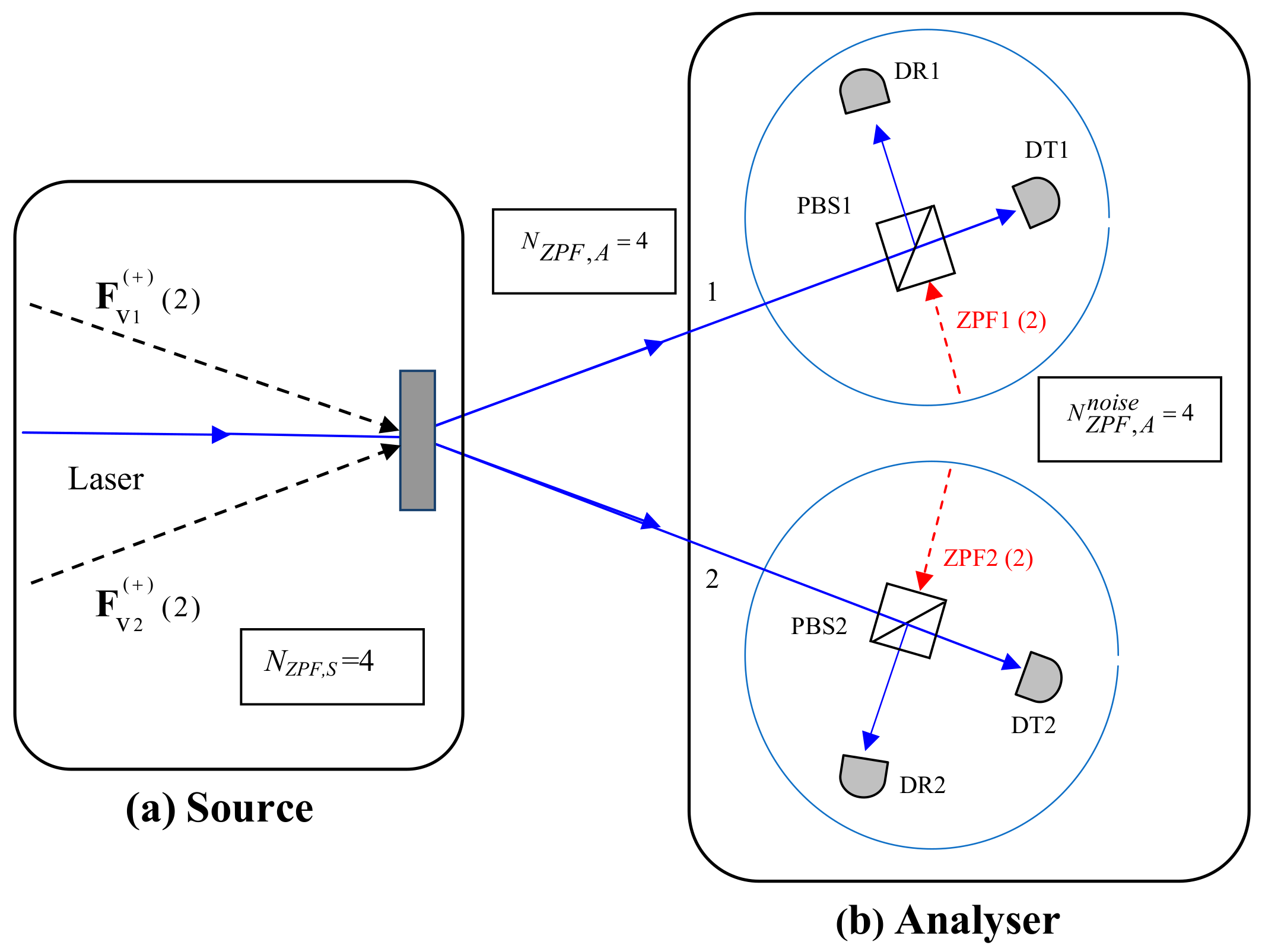
(
) represents the set of zeropoint amplitudes corresponding to the polarisation
of the entering zeropoint beam with wave vector
(see
Figure 1). The sets of zeropoint amplitudes that appear in each electric field component have been included for a better understanding of the correlation properties that characterise entanglement in the WRHP formalism. In Equations (
32) and (
33), the only non-vanishing cross-correlations are those concerning
and
, which is a consequence of Equations (
12)–(
14). On the other hand, the states
are described using the correlated beams [
33]:
where
(
) stands for
(
).
2.5. ZPF and the Limits on Optimal BSM
Bell-state analysis is a key aspect in quantum information [
41]. In optical communication, it is well-known that a complete distinguishability of the four Bell-states of two photons entangled in one degree of freedom (see Equations (
30) and (
31)) is not possible, by using only linear evolution and local measurement (LELM) [
42]. Hyperentanglement is a good resource for getting complete distinguishability [
43]. However, increasing the dimensionality of the Hilbert space also opens the possibility of exploring the capacity for maximal distinguishability.
This subject has brought about a lot of theoretical works, of which we summarise the main results [
44]. Let us consider two bosons entangled in
n dichotomic degrees of freedom. The dimension of the Hilbert space is
, and the maximal distinguishability of Bell-like states using LELM is bounded above by
: a single detection event at any of the
detectors does not discriminate Bell states, so that the maximal distinguishability is bounded by the
possibilities for the second detection. The maximum number of distinguishable Bell-states classes depends on the way in which the two particles propagate through the setup. If they are not brought together, the maximal distinguishability is
(each single detection area contains
detectors). If the two bosons interact at the apparatus, the maximum number of Bell-state classes that can be distinguished is equal to
. For instance, for
, the dimension of the Hilbert space is 4, the maximal distinguishability is equal to 2 if the two particles are not mixed at the apparatus, and 3 if they interact. Then, for
, it is not possible to distinguish the four Bell-states.
The original contribution of the WRHP approach to the subject of optical BSM is based on the counting of the different zeropoint inputs at the setup. Hyperentanglement implies the “activation” of a greater number of sets of ZPF modes at the source. As it has been proved elsewhere [
35], the upper bound to maximal distinguishability (
) just corresponds to the number of sets of ZPF modes that are amplified at the source of entanglement (
). On the other hand, measuring implies the existence of a fundamental noise inside the analyser, which limits the information that can be obtained. The zeropoint modes entering the idle channels inside the analyser must be subtracted, in an appropriate manner, to the number of sets of amplified ZPF modes entering the analyser, in order to obtain the maximal distinguishability.
If the two photons propagate from the source to the detectors via separated spatial channels, i.e., the photons do not interact, it has been demonstrated that the maximal distinguishability,
, is equal to the difference between the number of sets of amplified ZPF modes that enter the analyser,
, and the number of sets of ZPF modes entering the area corresponding to a single detection event,
, which is located inside the analyser. Hence,
where
coincides to
in the case in which there are no additional ZPF inputs between the source and the analyser (
=
=
). On the other hand,
with
=
being the total number of sets of ZPF modes that enter the idle channels inside the analyser. In this way,
This result coincides with the one predicted in [
44]. The case
n = 2 (polarisation–momentum hyperentanglement) has been studied with the WRHP approach in [
35]. On the other hand, Equation (
36) has been recently applied to the analysis of the four polarisation–momentum Bell-states corresponding to only one photon [
37].
3. Polarisation Entanglement, Zeropoint Field, and BSM
The motivation for this section comes from the following question: How do the ZPF amplitudes act in BSM, so that Equation (
36) is fulfilled in the case
? Let us consider the following basic setup. Four sets of ZPF amplitudes entering the crystal are amplified, giving rise to two correlated beams. Two polarising beam-splitters, PBS1 and PBS2, separate the horizontal and vertical components of the light fields, which are detected at DT1, DR1, DT2 and DR2 (see
Figure 2). The two sets of ZPF amplitudes entering the idle channels of each PBS are crucial. In this case,
=
= 4, and
= 4, in such a way that
= 2. It follows that
In this experiment, the first class corresponds to the states and . A joint detection can be produced at detectors DR1 and DT2, or DT1 and DR2. On the other hand, the second class contains the states and : the joint detection can be given at detectors DR1 and DR2, or DT1 and DT2. As a conclusion, this setup is unable to distinguish the value of .
The joint detection probabilities for this basic setup, calculated with the WRHP approach, can be consulted in [
33].
Let us now proceed to give a physical interpretation of Equation (
39) based on the role of the zeropoint amplitudes as “hidden” stochastic variables. For simplicity, we consider an identical distance separating the crystal from the respective PBSs and detectors, in such a way that the phase shift in Equation (
16) can be ignored. In addition, we take
=
in Equation (
19), so that the spacetime dependence is discarded. From Equations (
23), (
24), (
32) and (
33), we have:
where we have made the change
=
, in order to consider that the energy of the classical wave corresponding to the laser, which is proportional to the squared amplitude, must be divided into four amplitudes. On the other hand,
(
) stands for
(
), and
=
represents the vacuum beam entering the crystal with wave vector
. If we were considering the states
and
, Equation (
40) would not change, but the horizontal and vertical components should be exchanged in Equation (
41). Taking into consideration the zeropoint field entering the idle channel of each PBS, which transmits (reflects) horizontal (vertical) polarisation, the field amplitudes at the detectors DT1, DR1, DT2 and DR2, are:
where
=
represents the zeropoint beam entering the polarising beam-splitter PBSi. For the sake of clarity, we use the notation
for the vacuum fields entering the source, and “ZPF” for the corresponding ones entering the idle channels inside the analyser.
Let us calculate the intensity at the detectors. For simplicity, we consider that only four zeropoint modes enter the crystal, fulfilling the exact matching conditions, so that the operator
G (
J) can be replaced by 1 (
) [
19,
29]. By putting
V =
,
=
and
=
, the intensity at the detectors, retaining terms of order up to
, are:
where
and
Equations (
46)–(
49) correspond to the intensity of light at each detector in the case of
. If we were considering the states
, only
and
would change, by exchanging
and
in Equations (
48) and (
49). The single detection probability can be calculated by using Equation (
17). For instance, from Equations (
46) and (
51), we have:
where we have taken into account that
, which can be deduced from Equation (
11). Similar expressions hold for
,
and
, irrespective of the state. For this reason, a single detection event does not discriminate any of the four Bell states.
From Equations (
46)–(
49), the intensity above the threshold takes an identical value in DT1 and DR2 (DT2) (DR1 and DT2 (DR2)) for states
(
). The value of
does not appear in Equations (
46)–(
49) so that only two classes can be distinguished. The value of
depends on the crystal and the laser beam through the coupling parameter
, and the modulus and phase of two of the four vacuum amplitudes entering the crystal. Specifically, the wave coupling is represented by a first-order term in the parameter
g, which depends on the phase
given in Equation (
50).
We conjecture that detection in any of the four ideal detectors (
) would be produced when the vacuum amplitudes entering the crystal gave rise to constructive interference at the corresponding outgoing channel. For instance, if detection in, e.g., DT1, is produced in the case
, then the second detection event will occur in DR2 (DT2) in the case
(
). However, these two possibilities could be distinguished only by subtracting the total contribution of the zeropoint field entering PBS2, which is represented by the two sets of ZPF modes
and
. In fact, the stochastic intensity
(
) keep hidden the contribution of the vacuum amplitudes
and
(
and
) to the total intensity
(
). The difference,
= 2 (see Equation (
39)), which gives the maximal distinguishability in this experiment, is a proof of the visible presence of the vacuum field.
4. The Role of the Zeropoint Field in Quantum Cryptography
Quantum cryptography is based on the projection postulate and the compatibility theorem of quantum mechanics. The use of non-compatible observables in the send and reception of quantum information is the basic principle of the first protocol for quantum key distribution (QKD), known as BB84, that was developed by Bennett and Brassard in 1984 [
45]. Some years later, QKD based on entangled states was presented by Ekert in 1991 [
46]. This allowed the use of Bell’s inequalities in order to detect eavesdropping attacks in the case of projective measurements, which implies the introduction of hidden variables that destroy the quantum behaviour of the system.
Experiments on quantum cryptography using entangled photons generated in PDC have been analysed with the WRHP formalism [
33]. Although the Wigner formalism is purely quantum, its connection with SO gives rise to a new perspective that reinforces the crucial role of the zeropoint field. For instance, in the case of eavesdropping attacks, an essential ingredient is the noise introduced by Eve through the idle channels of their apparatuses, which gives rise to a change in the correlation properties of the light field. Hence, the hidden variables introduced during the attack can be identified to the zeropoint amplitudes entering the idle channels of the polarisers. In classical optics, where the intensities of light are so high that vacuum fluctuations can be neglected, the noise introduced by Eve does not have any influence. For this reason, attacks in classical cryptography can be made without being detected. In contrast, this noise is very important in quantum cryptography, and allows for the detection of the attack.
Let us now proceed to study the generation and measurement of linearly polarised signals with the WRHP approach, with the aim of investigating the role played by the vacuum field in the BB84 protocol. We consider the general case of signals described in Equation (
8). In classical optics, polarised light can be generated by using a linear polariser, so that the Malus law relates the outgoing and incoming intensities. Let us consider the action of a PBS. If a signal beam enters one of the channels, the light at each output channel is linearly polarised and the outgoing intensities are lower than the incoming one. However, if the intensity is decreased in such a way that only one photon can be detected, then the vacuum fluctuations become relevant. In the WRHP formalism, this implies that a zeropoint beam entering the idle channel of the PBS must be considered. For instance, a vertically polarised beam must be described by the sum of a signal (
) and the horizontal component of the ZPF (
):
The measurement of the polarisation in the diagonal basis can be accomplished by means of a half-wave-plate (HWP) and a PBS that transmits (reflects) horizontal (vertical) polarisation (see
Figure 3). The beam
leaving the HWP is:
On the other hand, to obtain the beams exiting the PBS, the vacuum field entering the idle channel,
, must be considered. We have:
Let us now calculate the total intensity at each of the outgoing channels,
and
. By putting
=
and
=
and by taking into account that
+
=
, the outgoing intensities are:
where
=
+
corresponds to the intensity entering the PBS. From the above equations, it can be seen that the intensity at each outgoing channel has an identical contribution,
, corresponding to the vertically polarised signal, and there is also an addend that represents the interference between
and
, with opposite values at each outgoing channel. Finally, there is a different contribution
(
), coming from the idle channel of the PBS, in the expression of
(
).
At this point, we should note that the intensity in each output channel can be greater than the corresponding one to the input, giving rise to
enhancement. This phenomenon is not produced in classical optics, where vacuum fluctuations do not have any influence. In contrast, enhancement is a key piece in SO [
47] and a basic ingredient of the wave-like description in the WRHP approach.
Let us now consider detection. It implies noise subtraction, i.e., the total contribution to the intensity coming from the zeropoint field itself must be subtracted. We have:
where
is the part of
corresponding to pure zeropoint field. The above equations explain
anticorrelation: detection (not detection) in one of the exit channels comes from a constructive (destructive) interference between the vertically polarised signal beam and the horizontal component of the zeropoint field that accompanies the signal. By performing an average with the Wigner function corresponding to the signal beam, and taking into account that
and
are uncorrelated, we obtain:
which implies an identical detection probability at each outgoing channel.
The uncertainty in the photon-path when different bases are chosen in the sending and reception of qubits is in the heart of secure KQD. In the WRHP approach, this is explained through anticorrelation at the exit channels, a typical effect based on wave interference, added to the consideration of a threshold for detection just at the zeropoint level.
5. The Meaning of Teleportation in Terms of the Zeropoint Field
At the end of the 1990s, quantum teleportation was achieved [
48,
49,
50]. Teleportation consists of transferring the quantum state of a two-state system
at a distant place, using Einstein–Podolsky–Rosen (EPR) entanglement of systems
and
and classical communication. A BSM on
and
gives Alice an information which, transmitted to Bob, allows him to manipulate
in order to put it in a state identical to the initial state of
. The Innsbruck experiment on teleportation was performed by means of two independent pairs of entangled photons, and one of the four photons as a trigger in order to prepare the state to be teleported [
49]. This scheme cannot be accomplished with
success due to the impossibility of a complete Bell-state analysis of two photons entangled only in one degree of freedom.
In contrast, in the Rome teleportation experiment, only two entangled photons are needed,
and
being replaced by two different properties of one photon, namely polarisation and momentum. One of these is teleported to the other photon in the pair [
50]. In the theoretical proposal of Popescu [
38], the two photons were entangled in momentum and polarisation was teleported. This experiment has been recently analysed with the Wigner formalism [
37]. We develop here this other version, used by Michler et al. [
51], taking advantage of the fact that photons produced in type-II PDC are already entangled in polarisation. A study of this experiment was done with the Wigner approach, with the aim of stressing the role of ZPF in teleportation [
52]. The significant contribution of this paper is that we analyse the mechanism leading to the fulfillment of Equation (
36) in one-photon polarisation–momentum BSM.
For the sake of clarity, we first analyse this experiment with the standard Hilbert space formalism. Let us consider the two-photon state:
where
H and
V represent the polarisation of the photons and
a and
b their momenta. The goal is to teleport the momentum degree of freedom from photon 1 to photon 2 by using their entanglement in polarisation. The Preparer uses a Mach–Zehnder interferometer in which the reflectivity
R (or the transmitivity
T) of the first beam-splitter and the phase
of the interferometer can be controlled at will. In this way, the momentum state of photon 1 becomes
After that, the resulting state of the two-photon system can be written by making use of the four-dimensional Bell-state basis of polarisation and momentum for photon 1 as
Alice detects photon 1 in one of its four possible states. Her analyser can consist of a set of three PBSs followed by four detectors (see
Figure 4). The two beams (represented by paths
and
) inside the different inputs of PBS1 (oriented in such a way that it transmits horizontal polarisation and reflects vertical). Each outgoing beam (represented by paths
and
) passes through a polarization analyser in the
basis, consisting of a half-wave-plate, a PBS, and two detectors. Now, depending on which of the four detectors (D1–D4) clicks, the state of photon 1 will collapse into one of its four possibilities expressed in Equation (
64). Alice informs Bob about her result. Bob, by making use of a quarter-wave-plate, a half-wave-plate, PBS4 (oriented like PBS1) and a polarisation rotator PR(90
), can always reconstruct the momentum state of photon 1.
In practice, to know whether teleportation has been successful, Bob’s signal enters a verification station. Beams concerning paths
and
come into the different inputs of a balanced beam-splitter BS2. By analysing coincidences between detectors D1 and D6 an interference pattern with the shape
should appear, where
C is a constant related with the efficiency of the detectors.
In the WRHP approach, the beams outgoing the crystal are given by Equations (
32) and (
33), by putting
. For simplicity, we discard the dependence on
and
t. Beam
(
) is sent to Alice (Bob). Now, beam
is passed through the Mach–Zehnder interferometer. The idle channel of BS1 constitutes a fundamental input of ZPF modes, in order to generate the superposition given in Equation (
63). By considering the action of mirrors M1, M2, and the zeropoint input beam
, the beams entering PBS1 are:
PBS1 transmits (reflects) horizontal (vertical) polarisation. The outgoing beams in paths
and
are:
In [
51],
(
) enter a polarising beam-splitter PBS2 (PBS3) that transmits (reflects) the diagonal polarisation at
(
). This is equivalent to consider the action of a half-wave-plate (with the optical axis at
) that rotates the polarisation plane of the beams
and
around the propagation direction, and that PBS2 (PBS3) transmits (reflects) horizontal (vertical) polarisation. The field amplitudes at the detectors D1, D2, D3 and D4 are:
where
and
represent the zeropoint beams entering the polarising beam-splitters PBS2 and PBS3.
Now, we analyse the verification measurements at Bob’s station. Beam
is passed through a polarising beam-splitter PBS4 that operates in the same way as PBS1, and the reflected beam enters a polarisation rotator that rotates
the polarisation in channel
. Then, the field amplitudes
and
entering BS2 are:
where
is the zeropoint field entering the idle channel of PBS4.
At this point, we analyse the cross-correlation properties of the light fields. The vacuum amplitudes entering the different polarising beam-splitters are uncorrelated with the signals and with each other. On the other hand, by taking into account that
=
(see Equation (
27)), we have:
The former equations contain the intrinsic nature of teleportation, which is mediated by the distribution of the ZPF amplitudes in each electric field component. By comparing Equations (
64) and (
75), we deduce that a photodetection at detector D1 would give rise to the teleportation of the prepared state to Bob’s photon. A detailed analysis of the reconstruction of the state in the WRHP approach can be consulted in [
37].
For the verification measurements, beams
and
enter a balanced non-polarising beam-splitter BS2. The field amplitudes at the detectors D5 and D6 are:
The joint detection probabilities are easily calculated by using Equation (
29) and by taking into account the correlation properties given by Equations (
75)–(
78). For instance, by considering the detector D1, we have:
and similar Equations hold for D2 by exchanging the + and − signs in Equations (
81) and (
82). Finally, the corresponding expressions concerning D3 (D4) are the same as for D1 (D2).
5.1. Hidden Variables and Complete One-Photon Polarisation–Momentum Bell-State Analysis
In this experiment,
is the number of sets of ZPF modes that are activated at the nonlinear crystal. The Preparer introduces two additional sets of ZPF modes through
, so that
. By taking into account that there are two idle channels inside the analyser, each introducing two sets of ZPF modes, we have
. By applying Equations (
36) and (
37), the maximal distinguishability is:
This result was demonstrated in [
37] by using a heuristic argument. Now, Equation (
83) is proved based on the consideration of the role of the ZPF amplitudes as hidden stochastic variables.
Let us calculate the total intensity corresponding to the exit channels of PBS1,
and
. By putting
,
,
and
, we have, by using Equations (
68) and (
69):
where
The phases of the signal beam, , and the zeropoint field entering the beam-splitter, , are coupled so that the light intensities and are anticorrelated: if two detectors were placed in channels and , each of them with a threshold just at the level of the zeropoint intensity, detection would happen only in one of the two channels.
The conditions for a constructive (destructive) interference in channel
(
) are:
and constructive (destructive) interference in channel
(
) implies:
From Equations (
87) and (
88), we deduce that the path choice of Alice’s photon is closely related to the coupling between the phases of the fields involved. Given that
and
are linear transformations of the zeropoint beams entering the crystal, Equations (
87) and (
88) involve the six sets of vacuum amplitudes entering the analyser (
).
Now, we obtain the intensities at the detectors D1, D2, D3 and D4. For instance, for detectors D1 and D2, concerning
, we have:
where
(
) stands for D1 (D2),
≡
and
≡
. In the same way, the intensities at the detectors D3 and D4 are:
where
() stands for D4 (D3), and .
From Equation (
89), it can be seen that the intensities at the detectors D1 and D2 contain three contributions: (i) the intensity of the transmitted or the reflected component of
; (ii) half of the total intensity at path
; and (iii) some addends, which depend on the phases
,
and
, given in Equations (
86) and (
90), with opposite values at the detectors D1 and D2. A similar reasoning holds for D3 and D4.
The intensities
and
, coming from the vacuum inputs entering PBS2 and PBS3 must be subtracted, along with the rest of addends involving pure ZPF contribution at each detector, in order to obtain the measurable intensity. From Equation (
89), it can be deduced that
(
) is maximum when Equation (
87) is fulfilled, along with the condition
(
). The same reasoning holds for detectors D3 and D4, so that
(
) is maximum when Equation (
88) is fulfilled, along with the condition
(
).
The values of
,
,
and
depend on the six sets of ZPF amplitudes entering the analyser, and the controllable experimental parameters
V,
g,
,
R,
T and
. Specifically, the phase
of the interferometer appears in the expressions of
and
. For a given value of these parameters, the hidden variables concerning
would define the path choice,
or
, of Alice’s photon exiting PBS1. Nevertheless, for a given path in which the intensity is maximum (see Equations (
84) and (
85)), the two possibilities concerning the detector to which the photon finally goes are hidden due to the noise coming from the ZPF entering the PBS before the detectors. These two possibilities could be distinguished only by subtracting the two sets of ZPF modes entering the corresponding detection area. This can be applied to any of the two paths exiting PBS1, so that the difference
gives the maximal distinguishability, and corresponds to the four polarisation–momentum Bell-states of the photon (see Equation (
83)). Let us emphasise that four represents the number of phases (
,
,
,
) that define the path choice of the photon from BS1 to the detectors, by subtracting the ZPF contribution at PBS2 and PBS3.
6. Discussion and Conclusions
In this paper, new results are presented that enhance the physical meaning of the vacuum field in optical quantum communication. These results have been obtained with the WRHP approach of QO, being consistent with the theory of SO based on the existence of a zeropoint field.
The underlying assumptions concerning the role of the zeropoint field in the arena of Bell-state analysis, along with the expressions that were heuristically obtained in previous works [
35,
37], have been confirmed by considering the role of the ZPF amplitudes as hidden variables (see
Section 3 and
Section 5.1). This represents an advance in the understanding of the internal mechanisms involving the propagation of the ZPF amplitudes through the setup, leading to the distinguishability of Bell-states.
In the Wigner formalism of QO, photodetection implies the subtraction of pure zeropoint field contribution to the light intensity. A part of this contribution comes from the noise entering the idle channels inside the analyser. The role of this noise in BSM is that the maximal distinguishability must be lower than the upper bound given by the number of sets of ZPF modes entering the analyser, in which the quantum information is stored. Given that the Wigner formalism is a bridge that connects QO to SO, the double role played by the ZPF as a store of information as well as as a fundamental limiting noise comes from the consideration of the vacuum field as a real stochastic field, irrespective of the problem of detection in SO (negative probabilities). What is remarkable is that the expressions that relate Bell-state distinguishability and zeropoint entries at the setup have been obtained by using a quantum formalism that resembles stochastic optics, just by adding the zeropoint field. These expressions have been demonstrated for experiments in which the two photons travel independently by the experimental setup, so that they do not interact. In further works, the general case, in which both photons are brought together at the setup, will be investigated.
Furthermore, the relationship between the compatibility theorem in QKD and zeropoint field has been emphasised. The projection postulate is an essential piece in secure quantum cryptography. Measuring implies the destruction of the vector state of the system, and this gives rise to the possibility of generating secure keys and detecting eavesdropping. In this sense, the compatibility theorem in quantum mechanics constitutes a basic ingredient in the BB84 protocol and other protocols for QKD. The analysis made in
Section 4 reinforces the role of the zeropoint field in optical quantum cryptography, and allows for a different point of view that is insides the internal mechanism leading to secure QKD.
A linearly polarised signal in the rectilinear basis must be superimposed to the orthogonal component of the ZPF. When this signal is measured in the diagonal basis, the phases of the signal and the ZPF are coupled, giving rise to anticorrelation at the output ports of the PBS. This anticorrelation explains that detection is produced only in one of the two detectors, once the contribution of the pure zeropoint intensity is subtracted. On the other hand, the zeropoint beam entering the idle channel of the PBS gives rise to enhancement, i.e., the total intensity at each of the outgoing channels can be greater than the incoming one. Enhancement and anticorrelation constitute two basic properties of the light description in SO [
8,
9]. In the WRHP formalism, these two differential features are linked to the preservation of the commutation rules of the electric field operator in unitary transformations [
33].


