Article

On the Classical Coupling between Gravity and Electromagnetism

1
Department of Physics & Astronomy, University of Nebraska-Lincoln, Lincoln, NE 68588, USA
2
Holland Computing Center, University of Nebraska-Lincoln, Lincoln, NE 68588, USA
*
Author to whom correspondence should be addressed.
Atoms 2015, 3(3), 320-338; https://doi.org/10.3390/atoms3030320
Submission received: 14 January 2015 / Revised: 30 May 2015 / Accepted: 17 June 2015 / Published: 30 June 2015

Abstract

:
Coupling between electromagnetism and gravity, manifested as the distorted Coulomb field of a charge distribution in a gravitational field, has never been observed. A physical system consisting of an electron in a charged shell provides a coupling that is orders of magnitude stronger than for any previously-considered system. A shell voltage of one megavolt is required to establish a gravitationally-induced electromagnetic force equal in magnitude to the force of gravity on an electron. The experimental feasibility of detecting these forces on an electron is discussed. The effect establishes a relation between Einstein’s energy-mass equivalence and the coupling between electromagnetism and gravity.

1. Introduction

Coupling between gravity and electromagnetism through the deflection of light around a massive object is a well-known effect. It was made popular by Einstein, who correctly predicted the angle of deflection of starlight around the Sun during a solar eclipse, verifying his general theory of relativity [1,2]. A less familiar example of coupling between gravity and electromagnetism is the distortion of electromagnetic fields in the presence of a gravitational field. The fields of point charges bend under the influence of gravity. This can be established by inspecting the fields of accelerating charges (Reference [3], Equations (14.13) and (14.14)) and applying the equivalence principle [4], which implies that the fields of a point charge at rest in a uniform gravitational field of strength g are identical to the fields of a point charge at rest in a uniformly-accelerating frame with upward acceleration g . The electric field lines are found to droop similar to the branches of a tree, and there is no magnetic field [5]. As a result, two neighboring charges held at equal heights experience a component of force in the vertical direction, as pointed out by Boyer [5]. This type of coupling between gravity and electromagnetism has never been observed.
Therefore, can gravity have an appreciable effect on electromagnetism? Griffiths pointed out that for two charges of opposite sign, electrostatic levitation, due to coupling between gravity and electromagnetism, is in principle possible, but experimentally inaccessible [6]. Rohrlich [7] and Boyer [5] have also stated that the distortion of the Coulomb field in a gravitational field is too small to be measured. To investigate this question, we consider an electron because it has a large charge-to-mass ratio, and instead of a second charged particle, we use a uniformly-charged spherical shell to increase the Coulomb energy. This system of an electron in a charged shell is depicted in Figure 1. It will be shown that there is an upward force on an electron positioned at the center of a positively-charged shell in the presence of a uniform gravitational field. This electric force can be made equal in magnitude to the gravitational force on the electron at a shell voltage of approximately 1 MV. Moreover, the electric force is gravitationally induced, and the balance is unaffected by the magnitude of the gravitational force. This feature distinguishes this phenomenon from others, such as magnetic, electric, acoustic and other forms of levitation [8,9,10]. Given that the observation of the free fall of electrons has been reported [11], it is clear that a demonstration of the coupling between electromagnetism and gravity in which the free fall of electrons is affected could be within reach experimentally.
Figure 1. Shell-charge system in a uniform gravitational field. This figure is an artistic representation of the effect of gravity on the electric fields of the shell. The electric field lines of the charged shell are shown in green, and equipotential lines are indicated in blue. The field inside the shell is much weaker than the field on the outside. The field lines on the inside convey the fact that, due to the presence of a uniform gravitational field, a uniform, vertical electric field is induced inside the shell [12]. Outside of the shell, the field lines droop downward. An electron (central white spot) is placed in the uniformly- and positively-charged shell (copper-colored sphere). At a shell voltage of about 1 MV, the electron will experience an upward, gravitationally-induced electric force that is balanced by its gravitational force.
Atoms 03 00320 g001
Starting from basic concepts, the model system is described, and an experiment is proposed in this paper. The following section will focus on the effect of gravity on electromagnetic fields. Section 3 investigates the interaction between two charged particles, referred to as an electric dumbbell [5,13]. This dumbbell model is extended to our proposed charged shell-electron system in Section 4. Our derivation is consistent with the self-force of a shell alone, which has been treated by Griffiths [13]. It will be shown that the classical calculation of the self-force for the proposed system exhibits the well-known 4/3 problem associated with the classical model of the electron [14,15,16,17,18,19,20,21,22,23,24,25]. This is expected, given that our charge distribution is spherically symmetric [26]. In Section 5, a brief historical account of this problem is provided. The experimental complication of charge redistribution is discussed in Section 6. Additionally, in Section 7, we discuss the experimental feasibility of observing a coupling between gravity and electromagnetism.

2. A Point Charge

In the absence of gravity, the electric field of a point charge is simply a Coulomb field. However, in the presence of a gravitational field, the Coulomb field becomes distorted. To describe this distortion, we first consider the “very strong principle of equivalence”, which states that “for every pointlike event in space-time, there exists a sufficiently small neighborhood such that in every local, freely falling frame in that neighborhood, all the laws of physics obey the laws of special relativity” [4]. This implies that laboratory size experiments performed in a uniformly-accelerating reference frame with upward acceleration g are indistinguishable from the same experiments performed in a non-accelerating reference frame that is in a uniform gravitational field of strength g . Therefore, the Liénard–Wiechert potentials for an accelerating point charge can be used to calculate the electromagnetic fields in an inertial frame, and the result can be extrapolated to a charge at rest in a gravitational field. The general expressions for the electromagnetic fields of an accelerating point charge q calculated from the Liénard–Wiechert potentials are:
E = q ( ( n ^ β ) ( 1 β 2 ) ( 1 n ^ · β ) 3 R 2 ) t r e t + q c ( n ^ × [ ( n ^ β ) × β ˙ ] ( 1 n ^ · β ) 3 R ) t r e t
B = ( n ^ × E ) t r e t
where n ^ is the unit vector pointing from the source point to the field point, β is the particle velocity divided by c , the speed of light,   R is the distance from the source point to the field point and t r e t is the retarded time [3]. Gaussian units are used in Equation (2.1), and they will continue to be used throughout the manuscript.
The gravitational field at the surface of the Earth is weak, static and nearly homogeneous across short distances. In this approximation, the field Equation (2.1) was used by Boyer to derive the electromagnetic fields of a point charge located at the origin of its rest frame in a uniform gravitational field to first order in g [5]. The magnetic field is zero, and the electric field is:
E ( x , y , z , t ) = q ( x 2 + y 2 + z 2 ) 3 / 2 [ i ^ ( x x 2 g c 2 y 2 g 2 c 2 z 2 g 2 c 2 ) + j ^ ( y x y g 2 c 2 )   + k ^ ( z x z g 2 c 2 ) ] .
In the derivation of Equation (2.2), the approximation to hyperbolic motion, β ˙ = ( g c ) x ^ , is used [5]. A plot of the electric field in Figure 2 provides a qualitative indication of how a gravitational field distorts the Coulomb field of a point charge [27].
Figure 2. Gravitationally-distorted Coulomb field of a point charge (blue point). The straight, black, dotted line indicates a horizontal field line when there is no gravity. The solid field lines are curved due to the presence of a vertical downward gravitational field g = 9.8  m / s 2 . At a horizontal distance of 10  cm (typical for table top experiments), the vertical component of the electric field E x is smaller than the horizontal component E y by a factor of 10 17 .
Atoms 03 00320 g002

3. An Electric Dumbbell

Now that we have a description of the electric field due to a point charge in a gravitational field, a second, identical particle is added to create an electric dumbbell. The electric dumbbell will be examined as a precursor to the system of interest, that is a charged particle inside a charged shell. In that system, each surface charge element of the shell, along with the central charged particle, form an electric dumbbell. A simple overview of the dumbbell is presented here, but the reader is referred to Boyer [5] and Griffiths [13] for detailed treatments of the system.
The electrostatic potential energy of the dumbbell is q 2 / d , where q is the charge of each particle and d is their separation distance. Einstein’s famous energy-mass equivalence relation suggests then that the mass of the two-particle system exceeds that of the sum of the two individual masses, by an amount:
m I = q 2 c 2 d .
If the dumbbell is placed in a gravitational field, the weight of the system will include a contribution from this interaction mass. It follows from the equivalence principle that the inertial mass of the system is also affected [4]. In fact, a recent experiment gave “the most precise direct test” of energy-mass equivalence of inertial mass using nuclear binding energies and atomic mass differences of different isotopes [28].
For the electric dumbbell, the electromagnetic forces between the two particles are no longer equal and opposite, but rather, there is a net force of the dumbbell on itself. For a dumbbell with horizontal orientation relative to the direction of the gravitational field, each individual point charge will experience a vertical component of force as a result of the distorted Coulomb field of the other charge (Figure 3). The vertical force experienced by one charge, F i ^ = q E i ^ , is equal to:
F = q 2 2 c 2 d g i ^ = 1 2 m I g i ^
where E i ^ is taken from Equation (2.2) with x = z = 0 and y = d . The entire system of two charges will then experience twice this force, effectively increasing the weight of the system by exactly the amount predicted by the energy argument. Thus, as Boyer showed, the increase in the weight of the system due to the interaction mass can be understood as the mutual electric forces between the charges [5].
If an arbitrarily-oriented dumbbell composed of different charges, q 1 and q 2 , is accelerated, the total self-force is given by F s e l f = ( q 1 q 2 c 2 d ) · [ a + ( a · d ^ ) d ^ ] , where d ^ is the direction of the dumbbell axis and a is the acceleration [13]. Defining ψ to be the angle d ^ makes with a , the component of F s e l f parallel to the acceleration a ,
F = ( q 1 q 2 a c 2 d ) ( 1 + cos 2 ψ )
is the purely inertial term from which the interaction mass, m I = q 1 q 2 c 2 d ( 1 + cos 2 ψ ) , is obtained. The force-derived interaction mass is dependent on the orientation of the dumbbell.
The forces experienced by the two charges can also be considered separately. The electric field Equation (2.2) is modified to describe the field of a point charge positioned at an arbitrary position ( x , y , z ) :
E ( x,y,z,t )= q [ ( xx ) 2 + ( yy ) 2 + ( zz ) 2 ] 3/2 { i ^ [ ( xx ) ( xx ) 2 g c 2   ( yy ) 2 g 2 c 2 ( zz ) 2 g 2 c 2 ]+ j ^ [ ( yy ) ( xx )( yy )g 2 c 2 ]   + k ^ [ ( zz ) ( xx )( zz )g 2 c 2 ]}
Taking only the field component parallel to the gravitational field, E i ^ , and expressing it in terms of the separation d = [ ( x x ) 2 + ( y y ) 2 + ( z z ) 2 ] 1 / 2 and angle ψ , where x x = d cos ψ , the force on one charge due to the other, F = q E i ^ , is:
F = q 1 q 2 d 2 [ cos ψ g 2 c 2 d ( 1 + cos 2 ψ ) ] i ^
The first term is the vertical component of an undistorted Coulomb field, and the second term gives the first-order correction to the Coulomb field in a gravitational field. When considering the force on the other charge, the angle ψ must be replaced with ψ + π . Thus, in a calculation of the total self-force of the system, the contribution of the first terms will cancel in accordance with Newton’s third law. Once again, we arrive at Equation (3.3) for the self-force of the dumbbell system.
Figure 3. Charged dumbbell. Two identical charged particles (blue points) in a gravitational field weigh more than the sum of their constituents. The excess mass, q 2 / c 2 d , follows from the energy mass equivalency. Boyer provided a force picture where the force due to curved field lines gives the same mass [5]. Only the field line connecting the two particles is depicted here. Each charge experiences both the downward gravitational force and the downward electric force.
Atoms 03 00320 g003

4. A Point Charge in a Charged Shell

Consider a spherical charged shell with a single charged particle at the center in a gravitational field. The electrostatic potential energy of the shell-charge system is found by calculating the work necessary to move the charge from infinity to the center of the shell. Taking the radius of the shell to be R and ignoring the energy needed to construct the shell, the electrostatic potential energy and energy-derived interaction mass of the system are:
U = q Q R  and  m I = q Q c 2 R
where Q = ρ   d a is the total charge of the shell.
Following the same procedure as for the dumbbell, we switch to a force argument, where the system is placed in a gravitational field. The central charge q and each infinitesimal charge element ρ  d a on the sphere’s surface constitute an electric dumbbell as described in the previous section. The vertical force on an infinitesimal charge element due to the central charge is given by:
d F ρ   d a = q ρ   d a R 2 [ cos θ g R 2 c 2 ( 1 + cos 2 θ ) ] i ^
where the field Equation (3.4) has been expressed in spherical coordinates. The spherical coordinate system is depicted in Figure 4. For a uniformly-charged shell, ρ is constant, and integration over the shell gives the total force on the shell due to the central charged particle:
F s = 2 3 q Q c 2 R g i ^
Likewise, the vertical force on the particle due to an infinitesimal charge element on the shell is given by:
d F q = q ρ   d a R 2 [ cos θ g R 2 c 2 ( 1 + cos 2 θ ) ] i ^
Integration gives the total force on the particle due to the shell: F q = F s . In the Appendix, the electric field is calculated along the entire vertical axis inside the shell, not just at the origin. The field is found to be constant for the entire vertical axis. Eriksen and Grøn have obtained the same result for the field using a different technique [12]. They show that the field is uniform throughout the entire interior of the shell to first order in g .
Figure 4. Coordinate system for the charged-shell charged-particle system. The particle (blue point) is positioned at the origin, which coincides with the center of the shell. The position of the area element d a of the shell is defined in terms of the angles θ and φ and the radius of the shell R. Gravity is in the negative x ^ direction.
Atoms 03 00320 g004
The force on the shell, F s , is identical to the force on the charged particle, F q , and the total self-force of the system is:
F t o t = 4 3 q Q c 2 R g i ^
This result can also be obtained by using Equation (3.3) to calculate the self-force of the shell-particle system where the angle ψ becomes θ and the integral is taken over the surface of the shell. The self-force-derived interaction mass of the shell-charge system is:
m I = 4 3 q Q c 2 R
which follows from Newton’s second law. However, a problem arises as we see that the force-derived mass is 4/3 that of the energy-derived mass.

5. The “4/3” Problem

In its early stages of development, particle electrodynamics consisted of macroscopic descriptions of particle-particle interactions (Coulomb’s law) and electromagnetic fields produced by charged particles and current sources (Maxwell’s equations). The work of Lorentz advanced the theory with a description of how charged particles respond to electromagnetic fields given by the famous expression F = q ( E + v c × B ) [14]. Lorentz’s goal was to account for macroscopic phenomena of electrodynamics in terms of the microscopic behavior of electrons and ions. His work, along with that of Abraham [15], even attempted to account for the structure of the electron. Their “classical” model of the electron consisted of a rigid spherical shell of uniformly-distributed charge density. However, several problems were soon identified with this model. Most relevant to our discussion is the 4/3 problem. Similar to the calculation for the charged particle in a charged shell system studied in the previous section, there is a 4/3 discrepancy between the self-force-derived mass and the energy-derived mass of the classical electron. We refer the reader to Griffiths for the detailed calculation [13]. Pearle has shown that by accounting for the proper time of each infinitesimal charge element in the self-force calculation, the 4/3 problem is resolved [16]. However, his calculation only applied to the special case of a spherically-symmetric shell. More recently, Ori and Rosenthal extended Pearle’s method to any charge configuration [17,18]. In the point-particle limit, they obtain Dirac’s covariant relativistic expression for the self-force of a point particle [19].
There also exists a 4/3 problem for the ratio of momentum-derived mass and energy-derived mass for the classical electron. This should not be confused with the self-force 4/3 problem under consideration thus far. Poincaré [20] and Rohrlich [21,22] each proposed an origin and corresponding resolution to the 4/3 problem for momentum-derived mass. Despite much debate regarding which of these resolutions is correct, it seems that there is no real incompatibility between them [13]. For our present discussion, the 4/3 factor [29] does not affect our conclusion.

6. The Complication of Charge Redistribution

So far, the material used to construct the spherical shell in the proposed model has not been specified. Experimentally, a convenient material is metal, because it is straightforward to apply a constant potential. However, if a conducting material is used, free charges will move under the influence of gravity, and there will no longer be a uniform charge distribution, as assumed in the analysis of the shell-charge system in Section 4. Thus, in this section, we consider the effect of gravity on the charged particles themselves rather than their fields.
A classical electrostatics description of a metal shell in a uniform gravitational field indicates that the conduction electrons will move in response to the gravitational field until the net force on them is zero. The shell is an equipotential surface after this sedimentation of electrons, and the total potential, which includes the electric and gravitational potentials, is a solution to Laplace’s equation. The details of the calculation can be found in the Appendix, Section A2. Inside the cavity of the shell, the electric field is found to be:
E = m e g e x ^
This field exerts a force on an electron that exactly opposes the force of gravity. Thus, a free electron inside the cavity feels no net force. Schiff and Barnhill obtained the same result for a metal drift tube using a quantum mechanical formalism [30].
A more thorough description of a conductor in a uniform gravitational field, given by Dessler, Michel, Rorschach and Trammell, includes the differentially-compressed lattice of positive ions in the metal, in addition to the sedimentation of conduction electrons [31]. Just as in the classical electrostatics approach, the metal surface is an equipotential surface. The reader is referred to [31,32] for the full calculation. The resulting “compression” electric field inside the cavity of the shell is:
E = ( m e g e + γ M g e ) x ^
where M is the atomic mass and γ is related to the material properties; specifically, it is regarded as the ratio of the elasticity modulus of the electron gas to that of the metal as a whole [31]. Dessler et al. estimated that the field inside a copper shell would be five orders of magnitude larger than the field predicted by Schiff and Barnhill and in the opposite direction [31]. A more modern prediction of γ for copper estimates that the field is 1500-times larger than the Schiff and Barnhill field and in the same direction [32]. The Dessler et al. field, given in Equation (6.2), is regarded as essentially correct; however, the values of γ are not fully understood theoretically [32].
This analysis of the gravitationally-induced electric field inside the cavity of a spherical conducting shell has not explicitly included coupling between gravity and electromagnetic fields. However, this is not expected to change the resulting field, because the condition of an equipotential surface must hold. Another feature of the electric field inside a conductor is that it is independent of the charge on the shell. This also results from the equipotential condition. Regardless of the total charge of the shell, the free charge will always redistribute in such a way so that a state of equilibrium is attained.
Establishing a uniform charge distribution is necessary if the resulting electric field inside the shell cavity is to be solely due to coupling between gravity and electromagnetism (i.e., curved field lines), as presented in Section 4. The preceding discussion of conducting shells suggests then that an insulating material, in which all charges are bound, should be used.

7. The Feasibility of Electron Free-Fall Experiments

We propose that a uniformly-charged, spherically-symmetric shell could be used, in principle, to demonstrate coupling between gravity and electromagnetism. The electric force on an electron, due to shell charge Q , along the vertical axis of the shell in a gravitational field is:
F e = 1 2 e Q c 2 R g i ^
where we have corrected the coefficient to account for the 4/3 problem. To reach a force equal in magnitude to the force of gravity on an electron, a shell voltage of:
V = Q R = 2 m e c 2 e = 1  MV
is required.
The coupling of gravitation and electromagnetism has been suggested by Griffiths as a means to levitate a dipole [6]. Griffiths’ dipole is equivalent to the electric dumbbell in Figure 3, except that the two point masses have equal, but opposite charge. As a result of being oppositely charged, the electric forces are directed upward, opposing the gravitational forces. Thus, levitation, where the electric force exactly balances the gravitational force, is, in principle, possible. In such a system, the levitation condition is dependent on the dipole separation. For dipole charges of ± e and a total mass twice that of an electron, levitation requires a separation distance of 1.4 × 10 15  m , half the classical electron radius. As Griffiths pointed out, this system is not experimentally accessible. The reason is that in an electron scattering experiment, the electrons stay within a distance of d = 10 15  m for only t = d v = d 2 q 2 / m e d ~ 10 23  s , in which time the effect of gravity cannot be measured with any current technique. Pushing two electrons together in a trap to a distance of 10 15  m requires trapping fields of 1  MV / 10 15  m and is also not experimentally accessible. Boyer also points out the difficulty in measuring the coupling between gravity and electromagnetism where the fractional distortion of the Coulomb field is on the order of 10 16 on Earth [5]. Even on a neutron star where g ~ 10 14  m / s 2 , the fractional distortion is still only 10 3 .
Realizing the charged-shell-electron system in the lab is less daunting, although still very challenging, as it would require the ability to observe electron free-fall. At the surface of the Earth, an electron experiences a gravitational potential gradient of m g = 5.6 × 10 11  eV / m . In a free-fall experiment for which the gravitational force on a single electron is dominant, all electric and potential gradients must be reduced to below this level.

7.1. Fairbank’s Experiments

William Fairbank and Fred Witteborn were the first to attempt an electron free-fall experiment [11,33,34,35]. Their experimental apparatus consisted of a vertical drift tube surrounded by a guide solenoid. A pulsed tunnel cathode at the bottom end of the tube served as the source of electrons. An electron multiplier positioned at the top enabled time-of-flight measurements from which the vertical force on the electron could be extrapolated. In addition to gravity, an adjustable vertical force was applied by passing current, vertically, through the drift tube walls. Variations in the work function across crystalline patches on the copper surface of the drift tube were expected to cause potential gradients on the order of 10 5 to 10 6   e V / m [34]. However, electron time-of-flight measurements indicated that all electromagnetic potential gradients were reduced to below 10 10  eV / m when the apparatus was cooled to below 4.5  K . This apparent reduction in potential variations was an unexpected result, but it turned out to be crucial for the success of the Witteborn–Fairbank (WF) electron free-fall experiment.
The results of the WF experiment were consistent with the presence of only one force, that of the applied electric field, acting on the electrons in the free-fall region of the drift tube. In the absence of an applied field, they measured a field value of zero to within ± 6 × 10 12  V / m [35]. Apparently, the gravitational force was cancelled by some other effect. This result was consistent with the prediction of Schiff and Barnhill that conduction gas electrons in a vertical metal tube would experience sedimentation resulting in an electron density gradient [30]. They calculated a resulting field of E = m e g / e directed downwards. This is the same field found for the shell in Equation (6.1).
Following publication of the WF results, Dessler, Michel, Rorschach and Trammell used an alternative treatment to calculate the gravitationally-induced electric field in metal. As discussed in the previous section, they considered the differentially-compressed lattice of positive ions in the metal, in addition to the sedimentation of conduction electrons [31]. Their result differed from that of Schiff–Barnhill in direction and by about five orders of magnitude; however, it did reduce to the Schiff–Barnhill result in the case of an incompressible lattice [31]. For copper, the Dessler et al. calculation predicts fields on the order of ~ 10 7  V / m [31]. Although there was no experimental evidence for this effect at the time, it seemed conceivable that these fields were simply being shielded by the same effect that was shielding the patch fields [11,31].
To better understand the apparent surface shielding observed in the WF experiment, the same apparatus was used to conduct free-fall experiments at temperatures ranging from 4.2 to 300  K [36]. At 300  K , the field was measured to be 7 × 10 6  V / m . A sharp transition in the field strength occurred below 4.5  K . At 4.2  K , the field was found to be smaller than 2 × 10 9  V / m , which was claimed to be consistent with the earlier measurement of 6 × 10 11  V / m . At the time of publication of these results, Lockhart et al. assumed that surface electrons on a layer of copper oxide ~ 20  Å thick on the inner surface of the drift tube were responsible for the shielding effect. However, there was, and still is, no theoretical model for this highly temperature-dependent shielding effect.
The possibility of a low-temperature shielding layer had been suggested by John Bardeen during an invited session of an American Physical Society meeting in 1968 [34]. Later, he proposed that an oxide layer on the surface undergoes a phase transition to a metallic state at 4.2  K , resulting in a positive surface charge and a two-dimensional conducting layer. The phase transition causes surface electrons to all come to the same electrostatic potential, and as a result, the fields outside the surface layer are reduced by several orders of magnitude. The reader is referred to [34] for a full account of Bardeen’s proposal.
The shielding effect, on which Fairbank’s electron free-fall measurement depends, has never been experimentally reproduced or theoretically understood, bringing into question the result [32]. However, in this context, it is interesting to note the results of Deslauriers et al. [37]. In experiments using trapped atomic ions as entangled quantum states, heating of trapped ions has been identified as an important source of decoherence. Deslauriers et al. found that cooling the trap electrodes from 300  K to 150  K resulted in a drop in ion heating by an order of magnitude or more. They state that, “these observations provide direct evidence that anomalous heating of trapped ions indeed originates from microscopic patch potentials, whose fluctuations are thermally driven and can be significantly suppressed by modest cooling of the electrodes” [37]. This result may be related to the “shielding” effect seen by Fairbank.

7.2. Modern Advancements in Technology

The WF experiments used electrons with energies less than 10 10  eV . Detection of single electrons was achieved with an electron multiplier. Counts were stored according to the elapsed time and recorded in intervals of 2.5  ms [11]. For an electron with energy equal to 10 10  eV (velocity 5.9  m / s ), the change in time-of-flight due to the force of gravity over a vertical flight path of 1  m is 34  ms . We consider now the feasibility of conducting an electron free-fall experiment with modern technology. Recent advancements are capable of providing much higher temporal resolution, making it possible to work at much higher electron energies than were used in the WF experiment. In fact, the effects of ambient fields could be reduced to the point that the unexplained shielding of patch potentials, which was never reproduced [32], would not be needed.
Consider an electron with energy 10 3  eV (velocity 1.9 × 10 4  m / s ). While it can be experimentally challenging to work with electrons at this energy, there are, for example, electron-molecule collision experiments that readily operate at or near this regime [38]. In the absence of any force, a 1  MeV electron would take 53  μs to travel 1  m . Now, consider this same electron at the Earth’s surface. The expected change in time-of-flight due to the force of gravity over 1  m is 0.74 × 10 12  s . Thus, any experiment designed to detect the force of gravity on a 1  MeV electron must have resolution better than a picosecond.
This resolution may be accessible, as fast sources capable of delivering sub- 100  fs pulses with <1 electron/pulse have been demonstrated [39,40]. Electron detectors currently on the market can reach a resolution of 30  ps [41]. However, detection schemes that use ultrafast phenomena in nanoscale structures allow for electronic switching times of 1  fs [42]. Plasmonic antennae (arrays of gold nanorods) have been shown to have an optical response faster than 20  fs [43]. It has been proposed that such a device, which exhibits near-field enhancement of the electric field, could be used as a femtosecond electron switch [43]. A system composed of a fast electron source and a femtosecond electron switch in conjunction with a standard multichannel plate could provide temporal resolution on the order of 100  fs . Furthermore, at 1  MeV , the electron’s velocity would be about two orders of magnitude above the expected shift in velocity due to patch potentials.
There is an additional complication in using a 100  fs pulse; the Heisenberg uncertainty principal dictates that it must have an energy spread no smaller than 3.3  MeV . To select a smaller energy spread, electron pulse compressors are becoming available with appropriate pulse duration, but currently, they only work at high (> keV ) energies [44]. Nevertheless, it may be possible to use laser pulses to select the electron flight time and reach a high time resolution [45,46].
Thus, advances in technology since the WF experiment could eliminate dependence on the surface shielding effect, and now may be the time for electron free-fall experiments to be reconsidered. Such free-fall experiments may serve to investigate the Dessler et al. field (Equation (6.2)), including the values of γ , which are not well understood theoretically.

7.3. Anticipated Difficulties

Charged particles readily couple to their environment through electric and magnetic fields, their gradients, radiation and residual gas scattering [32]. All of these interactions must be considered in the design and analysis of any free-fall experiment. The work in [32] provides an in-depth study of these experimental problems in the context of the WF experiment, including the complication of charge redistribution discussed in Section 6. In this work we propose to use 1  MeV electron energies, as opposed to the ~ 10 10  eV energies used in the WF experiment. Here, we reconsider two of the experimental requirements considered by Darling et al. that illustrate the point that higher energies are much easier to work with.
Collisions with residual gas particles can significantly affect time-of-flight measurements; thus, adequate vacuum pressures must be attained, such that the mean free path, l = ( σ n ) 1 , of the electron is greater than the length of the drift tube, where σ is the cross-section and n is the residual gas density. The cross-section for 1  MeV electrons interacting with nitrogen gas is σ = 9.85 × 10 16   cm 2 [47]. For a drift tube length of 1  m and temperature T = 300  K , the pressure, P = n k B T , must be less than 10 4  Torr , where k B is the Boltzmann constant. This pressure is readily attainable and much higher than the pressure of 10 12  Torr required in the WF experiment.
A solenoid magnetic field was used by WF to guide electrons down the axis of the drift tube, thus eliminating the effects of image charges. In order to limit interactions with magnetic field gradients, they used only electrons in the ground Landau state [11]. To load the lowest Landau state, a pinhole aperture can be used at the entrance to the uniform magnetic field region, such that its diameter (and thus, the width of the electron wave packet) matches the width of the lowest Landau state [48,49]. Thus, the projection of the electron wavefunction onto the ground Landau state is maximized. The separation between the electron source and the pinhole must also be chosen so that the pinhole is coherently illuminated [50]. For a 1  MeV electron and aperture diameter of 100  nm , the lowest Landau state can be loaded maximally for a source to aperture distance of 10  μm and magnetic field B = 3.6   G . These parameters can be experimentally attained with current technology.
As discussed in Section 6, gravity causes charges in a conductor to redistribute. The resulting compression field, given in Equation (6.2), would effectively mask the electric field due to the gravitational deflection of electric field lines. Thus, it may be necessary to use an insulating shell in the proposed experiment. Placing 1 MV on an insulating shell is a regime that to our knowledge has not yet been explored. The very fact that charges are not free to move on an insulator makes establishing a uniform charge distribution experimentally difficult. Whether or not it is possible to achieve highly uniform charge distributions on insulating materials is unknown to the authors at the time of writing this manuscript. Control parameters are likely to include the shape, surface preparation and size of the sphere. It is clear that some experimental feasibility study is necessary before embarking on the full proposed experiment.

8. Conclusions

While the classical coupling mechanism between gravity and the fields of a charge distribution is theoretically well established, no experiments have been performed to confirm the coupling. The proposed system of an electron inside a uniformly-charged shell increases the strength of the coupling significantly as compared to previously-discussed physical systems. The charged shell would affect the free-fall acceleration of electrons by an amount of g . This means that if electron free-fall can be observed, as previously reported by Fairbank et al., the effect of the coupling is also within experimental reach. Previous free-fall measurements relied on an unexplained shielding effect. The development of new ultrafast electron technology appears to remove the need to rely on this shielding effect. In contrast to earlier claims that the effect is too small to be observed, our discussion supports the view that now may be an opportune time to consider such experiments if the difficulty of uniformly charging an insulator can be overcome. Alternatively, free-fall experiments could be performed in metal drift tubes to investigate the gravitationally-induced electric field predicted by Dessler et al.

Appendix

In order to perform an experiment that is sensitive to the curvature of electric field lines using a charged shell as proposed in this manuscript, one must first be capable of performing electron free-fall measurements. In such an experiment, the electron would move along the vertical axis in the interior cavity of the shell. In this section, the electric field along the vertical axis is calculated for two cases: a uniformly-charged shell and a conducting shell with a non-uniform charge distribution. Consideration of a non-uniform surface charge density is motivated in Section 6.

A1. Uniformly-Charged Shell

For a shell with uniform charge density σ and total charge Q = 4 π R 2 σ , the vertical component of the electric field at any point ( x , y , z ) in the interior of the shell is given by:
E x ( x , y , z ) = σ [ ( x R cos θ ) g c 2 ( x R cos θ ) 2 g 2 c 2 ( y R cos φ sin θ ) 2 g 2 c 2 ( z R sin φ sin θ ) 2 ] [ ( x R cos θ ) 2 + ( y R cos φ sin θ ) 2 + ( z R sin φ sin θ ) 2 ] 3 / 2 d a
where d a = R 2 sin θ d θ d φ . This follows from Equation (3.4) when the source position is written in spherical coordinates according to Figure 4. Along the vertical x -axis, y = z = 0 , and the field expression reduces to:
E x ( x,y,z ) = σ [ ( xRcos θ ) g c 2 ( xRcos θ ) 2 + g 2 c 2 ( Rcos φ sin θ ) 2 + g 2 c 2 ( Rsin φ sin θ ) 2 ] [ ( xRcos θ ) 2 + ( Rcos φ sin θ ) 2 + ( Rsin φ sin θ ) 2 ] 3 2 d a     = σ [ ( x g x 2 c 2 g R 2 2 c 2 ) + ( 2 g R x c 2 R ) cos θ g R 2 2 c 2 cos 2 θ ] [ ( x R cos θ ) 2 + ( R cos φ sin θ ) 2 + ( R sin φ sin θ ) 2 ] 3 / 2 d a    = σ 0 2 π 0 π [ ( x g x 2 c 2 g R 2 2 c 2 ) + ( 2 g R x c 2 R ) cos θ g R 2 2 c 2 cos 2 θ ] [ R 2 + x 2 2 R x cos θ ] 3 / 2 R 2 sin θ d θ d φ     =2πσ R 2 [ A 0 π sin θ d θ [ R 2 + x 2 2Rxcos θ ] 3 2 +B 0 π sin θ cos θ d θ [ R 2 + x 2 2Rxcos θ ] 3 2        +C 0 π sin θ cos 2 θ d θ [ R 2 + x 2 2Rxcos θ ] 3 2 ]
where A = ( x g x 2 c 2 g R 2 2 c 2 ) , B = ( 2 g R x c 2 R ) and C = g R 2 2 c 2 .
Applying the substitutions u = cos θ and d u = sin θ d θ gives:
E x ( x , y , z ) = 2 π σ R 2 [ A 1 1 d u [ R 2 + x 2 2 R x u ] 3 2 + B 1 1 u   d u [ R 2 + x 2 2 R x u ] 3 2   + C 1 1 u 2 d u [ R 2 + x 2 2 R x u ] 3 2 ]
The solutions to the integrals are [51]:
1 1 d u [ R 2 + x 2 2 R x u ] 3 2 = 2 2 R x R 2 + x 2 2 R x u | 1 1 = 2 R ( R 2 x 2 )
1 1 u   d u [ R 2 + x 2 2 R x u ] 3 2 = 4 ( R 2 + x 2 ) 2 ( 2 R x u ) ( 2 R x ) 2 R 2 + x 2 2 R x u | 1 1 = 2 x R 2 ( R 2 x 2 )
and:
1 1 u 2 d u [ R 2 + x 2 2 R x u ] 3 2     = 2 ( 8 ( R 2 + x 2 ) 2 + 4 ( R 2 + x 2 ) ( 2 R x ) u + ( 2 R x ) 2 u 2 ) 3 ( 2 R x ) 3 R 2 + x 2 2 R x u | 1 1     = 4 x 2 + 2 R 2 3 R 3 ( R 2 x 2 )
Substituting these expressions back into Equation (A.3) gives:
E x ( x , y , z ) = 2 π σ R 2 [ ( x g x 2 c 2 g R 2 2 c 2 ) 2 R ( R 2 x 2 ) + ( 2 g R x c 2 R ) 2 x R 2 ( R 2 x 2 )   g R 2 2 c 2 4 x 2 + 2 R 2 3 R 3 ( R 2 x 2 ) ]
which reduces to:
E x = 2 3 Q g c 2 R
when the appropriate substitution for σ is used. Thus, the electric field is constant along the vertical axis inside a charged shell with a uniform surface charge density.

A2. Conducting Shell with Non-Uniform Charge Density

In a conducting material, free electrons will move in response to the gravitational field until the net force on them is zero:
F G + F E = F T = 0
Here, F G is the gravitational force, F E is the electric force and F T is the total (i.e., net) force on conduction electrons. Each of these forces is associated with a potential:
F G = V G
F E = V E
F T = ( V G + V E ) = V T
Since the net force is zero within the wall of the shell and at its surfaces, it follows that the total potential, V T , must be constant at these locations.
Next, observe that the gravitational potential, V G = m e g x , is a solution of Laplace’s equation:
2 V G = · ( V G ) = · ( m e g x ^ ) = 0
Since the gravitational force is constant and uniform in the x ^ direction, it follows from Equation (A.9) that the electric force must be, as well. As a result, the electric potential is also a solution of Laplace’s equation. The total potential, V T , which is a linear combination of V G and V E , must, then, also satisfy Laplace’s equation.
2 V T = 2 ( V G + V E ) = 0
The potential inside the cavity of the shell is determined using the fact that Laplace’s equation tolerates no local maxima or minima; extreme values of the potential must occur at the boundary [52]. It follows that the total potential inside the cavity is the same as the potential at the shell surface. Thus, an electron inside the cavity would experience an electric force that would exactly balance the gravitational force. The electric field inside the cavity of the shell is given by:
E = m g e x ^

Acknowledgments

Maria Becker, Adam Caprez, and Herman Batelaan gratefully acknowledge funding from NSF Grant Numbers 0969506 and 1306565. Maria Becker also gratefully acknowledges funding from the DOE GAANN Program Numbers 59954 and 68246.

Conflicts of Interest

The authors declare no conflict of interest.

References and Notes

  1. Einstein, A. The foundation of the general theory of Relativity. In The Principle of Relativity; Dover: New York, NY, USA, 1952; p. 163. [Google Scholar]
  2. Dyson, F.W.; Eddington, A.S.; Davidson, C. A determination of the deflection of light by the Sun’s gravitational field, from observations made at the total eclipse of 29 May 1919. Philos. Trans. R. Soc. 1920, 220A, 291–333. [Google Scholar] [CrossRef]
  3. Jackson, J.D. Classical Electrodynamics, 3rd ed.; Wiley: New York, NY, USA, 1999; p. 664. [Google Scholar]
  4. Ciufolini, I.; Wheeler, J.A. Gravitation and Inertia; Princeton University Press: Princeton, NJ, USA, 1995; p. 14. [Google Scholar]
  5. Boyer, T.H. Electrostatic potential energy leading to a gravitational mass change for a system of two point charges. Am. J. Phys. 1979, 47, 129–131. [Google Scholar] [CrossRef]
  6. Griffiths, D.J. Electrostatic levitation of a dipole. Am. J. Phys. 1986, 54, 744. [Google Scholar] [CrossRef]
  7. Rohrlich, F. Classical Charged Particles, 3rd ed.; World Scientific: Hackensack, NJ, USA, 2007; p. 219. [Google Scholar]
  8. Simon, M.D.; Geim, A.K. Diamagnetic levitation: Flying frogs and floating magnets. J. App. Phys. 2000, 87, 6200–6204. [Google Scholar] [CrossRef]
  9. Rhim, W.; Chung, S.K.; Barber, D.; Man, K.F.; Gutt, G.; Rulison, A.; Spjut, R.E. An electrostatic levitator for high-temperature containerless materials processing in 1-g. Rev. Sci. Instr. 1993, 64, 2961–2970. [Google Scholar] [CrossRef]
  10. Trinh, E.H. Compact acoustic levitation device for studies in fluid dynamics and material science in the laboratory and microgravity. Rev. Sci. Instr. 1985, 56, 2059–2065. [Google Scholar] [CrossRef]
  11. Witteborn, F.C.; Fairbank, W.M. Experiments to determine the force of gravity on single electrons and positrons. Nature 1968, 22, 436–440. [Google Scholar] [CrossRef]
  12. Eriksen, E.; Grøn, Ø. Electrodynamics of hyperbolically accelerated charges V. the field of a charge in the Rindler space and the Milne space. Ann. Phys. 2004, 313, 147–196. [Google Scholar] [CrossRef]
  13. Griffiths, D.J.; Owen, R.E. Mass renormalization in classical electrodynamics. Am. J. Phys. 1983, 51, 1120–1126. [Google Scholar] [CrossRef]
  14. Lorentz, H.A. The Theory of Electrons and Its applications to the Phenomena of Light and Radiant Heat, 2nd ed.; Dover Publications, Inc.: New York, NY, USA, 1952. [Google Scholar]
  15. Abraham, M. Prinzipien der Dynamik des Elektrons. Ann. Phys. 1903, 10, 105–179. [Google Scholar] [CrossRef]
  16. Pearle, P. Electromagnetism: Paths to Research; Teplitz, D., Ed.; Plenum: New York, NY, USA, 1982; Chapter 7. [Google Scholar]
  17. Ori, A.; Rosenthal, E. Universal self-force from an extended object approach. Phys. Rev. D 2003, 68, 041701. [Google Scholar] [CrossRef]
  18. Ori, A.; Rosenthal, E. Calculation of the self force using the extended-object approach. J. Math. Phys. 2003, 45, 2347–2364. [Google Scholar] [CrossRef]
  19. Dirac, P.A.M. Classical theory of radiating electrons. Proc. R. Soc. Lond. A 1938, 167, 148–169. [Google Scholar] [CrossRef]
  20. Poincaré, H. On the dynamics of the electron. Rend. Circ. Mat. Pulermo 1906, 21, 129–176. [Google Scholar] [CrossRef]
  21. Rohrlich, F. Electromagnetic momentum, energy, and mass. Am. J. Phys. 1970, 38, 1310–1316. [Google Scholar] [CrossRef]
  22. Rohrlich, F. Self-energy and stability of the classical electron. Am. J. Phys. 1960, 28, 639–643. [Google Scholar] [CrossRef]
  23. Rohrlich, F. The dynamics of a charged sphere and the electron. Am. J. Phys. 1997, 65, 1051–1056. [Google Scholar] [CrossRef]
  24. Yaghjian, A.D. Relativistic Dynamics of a Charged Sphere; Springer-Verlag: Berlin, Germany, 1992. [Google Scholar]
  25. Rohrlich, F. Classical Charged Particles, 3rd ed.; World Scientific: Hackensack, NJ, USA, 2007; Ch2; pp. 8–24. [Google Scholar]
  26. Jackson, J.D. Classical Electrodynamics, 3rd ed.; Wiley: New York, NY, USA, 1999; Section 16.3; pp. 750–757. [Google Scholar]
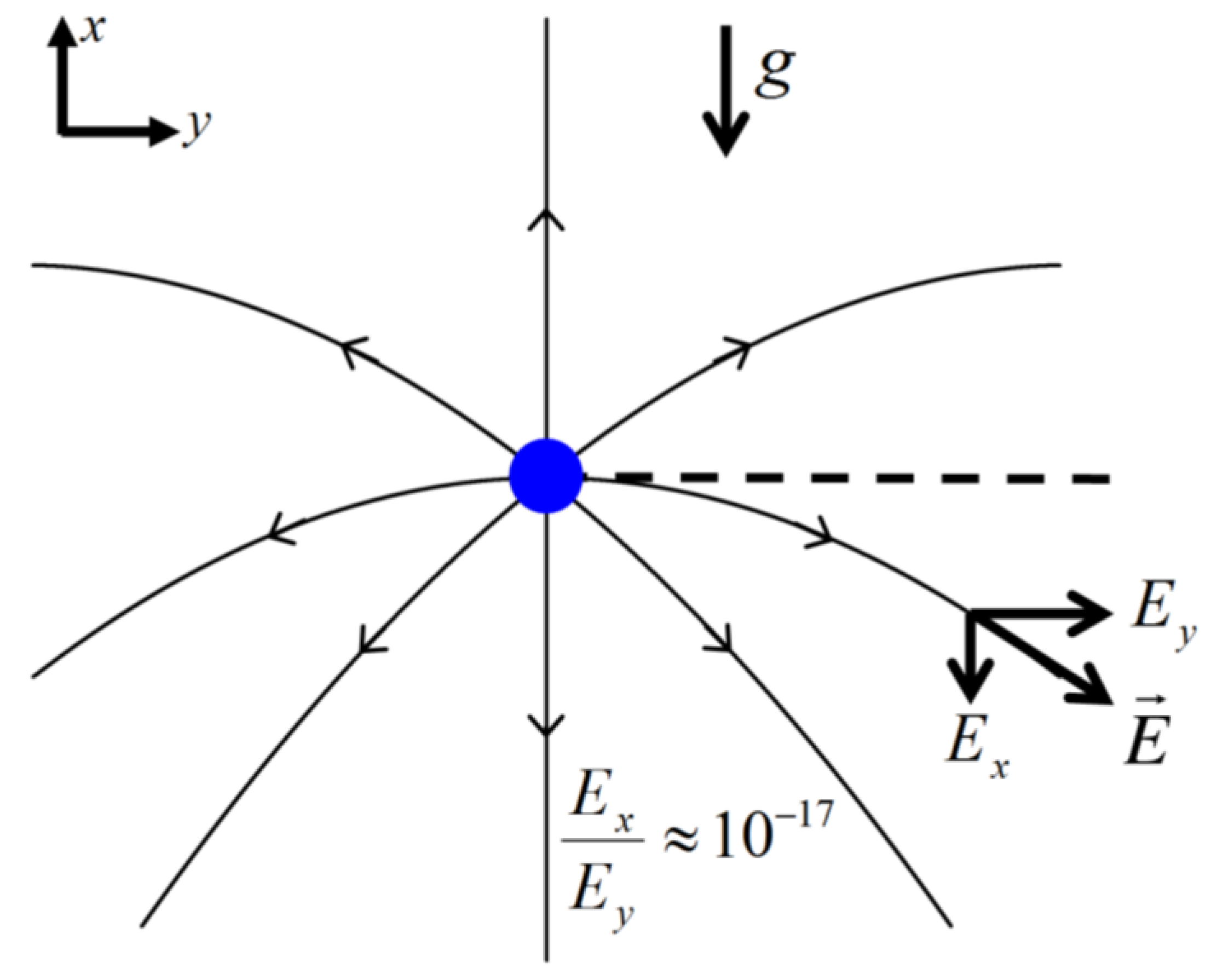
  27. In the introduction, the deflection of light in a gravitational field was mentioned, and now we have an expression for the deflection of electric field lines. It is interesting to note that electric field lines and light ray trajectories in a gravitational field have the same shape.
  28. Rainville, S.; Thompson, J.K.; Myers, E.G.; Brown, J.M.; Dewey, M.S.; Kessler, E.G., Jr.; Deslattes, R.D.; Börner, H.G.; Jentschel, M.; Mutti, P.; et al. World Year of Physics: A direct test of E = mc2. Nature 2005, 438, 1096–1097. [Google Scholar] [CrossRef] [PubMed]
  29. Many other notable contributions have been made towards resolving to the 4/3 problems that have not been mentioned here. For more extensive discussions on the theory of the classical electron the reader is referred to References [16,23,24,25].
  30. Schiff, L.I.; Barnhill, M.V. Gravitation-Induced Electric Field near a Metal. Phys. Rev. 1966, 151, 1067–1071. [Google Scholar] [CrossRef]
  31. Dessler, A.J.; Michel, F.C.; Rorschach, H.E.; Trammell, G.T. Gravitationally Induced Electric Fields in Conductors. Phys. Rev. 1968, 168, 737–743. [Google Scholar] [CrossRef]
  32. Darling, T.W.; Rossi, F.; Opat, G.I.; Moorhead, G.F. The fall of charged particles under gravity: A study of experimental problems. Rev. Mod. Phys. 1992, 64, 237–257. [Google Scholar] [CrossRef]
  33. Witteborn, F.C.; Fairbank, W.M. Experimental Comparison of the Gravitational Force on Freely Falling Electrons and Metallic Electrons. Phys. Rev. Lett. 1967, 19, 1049–1052. [Google Scholar] [CrossRef]
  34. Fairbank, J.D.; Deaver, B.S., Jr.; Everitt, C.W.F.; Michelson, P.F. Near Zero: New Frontiers of Physics; W.H. Freeman and Company: New York, NY, USA, 1988; Chapter 7. [Google Scholar]
  35. Witteborn, F.C.; Fairbank, W.M. Apparatus for measuring the force of gravity on freely falling electrons. Rev. Sci. Instrum. 1977, 48, 1–11. [Google Scholar] [CrossRef]
  36. Lockhart, J.M.; Witteborn, F.C.; Fairbank, W.M. Evidence for a Temperature-Dependent Surface Shielding Effect in Cu. Phys. Rev. Lett. 1977, 38, 1220–1223. [Google Scholar] [CrossRef]
  37. Deslauriers, L.; Olmschenk, S.; Stick, D.; Hensinger, W.K.; Sterk, J.; Monroe, C. Scaling and suppression of anomalous heating in ion traps. Phys. Rev. Lett. 2006, 97, 103007. [Google Scholar] [CrossRef] [PubMed]
  38. Graupner, K.; Field, T.; Mayhew, C.A.; Hoffmann, T.H.; May, O.; Fedor, J.; Allan, M.; Fabrikant, I.I.; Illenberger, E.; Braun, M.; et al. Low-Energy Attachment to the Dichlorodifluoromethane (CCl2F2) Molecule. J. Phys. Chem. A 2010, 114, 1474–1484. [Google Scholar] [CrossRef] [PubMed]
  39. Barwick, B.; Corder, C.; Strohaber, J.; Chandler-Smith, N.A.; Uiterwaal, C.J.; Batelaan, H. Laser-induced ultrafast electron emission from a field emission tip. New J. Phys. 2007, 9, 142. [Google Scholar] [CrossRef]
  40. Hommelhoff, P.; Kealhofer, C.; Kasevich, M.A. Ultrafast Electron Pulses from a Tungsten Tip Triggered by Low-Power Femtosecond Laser Pulses. Phys. Rev. Lett. 2006, 97, 247402. [Google Scholar] [CrossRef] [PubMed]
  41. Kiesel, H.; Renz, A.; Hasselbach, F. Observation of Hanbury Brown—Twiss anticorrelations for free electrons. Nature 2002, 418, 392–394. [Google Scholar] [CrossRef] [PubMed]
  42. Schiffrin, A.; Paasch-Colberg, T.; Karpowicz, N.; Apalkov, V.; Gerster, D.; Mühlbrandt, S.; Korbman, M.; Reichert, J.; Schultze, M.; Holzner, S.; Barth, J.V.; et al. Optical-field-induced current in dielectrics. Nature 2013, 493, 70–74. [Google Scholar] [CrossRef] [PubMed]
  43. Becker, M.; Huang, W.C.-W.; Batelaan, H.; Smythe, E.J.; Capasso, F. Measurement of the ultrafast temporal response of a plasmonic antenna. Ann. Phys. 2013, 525, L6–L11. [Google Scholar] [CrossRef]
  44. Van Oudheusden, T.; Pasmans, P.L.E.M.; van der Geer, S.B.; de Loos, M.J.; van der Wiel, M.J.; Luiten, O.J. Compression of Subrelativistic Space-Charge-Dominated Electron Bunches for Single-Shot Femtosecond Electron Diffraction. Phys. Rev. Lett. 2010, 105, 264801. [Google Scholar] [CrossRef] [PubMed]
  45. Freimund, D.L.; Aflatooni, K.; Batelaan, H. Observation of the Kapitza-Dirac effect. Nature 2001, 413, 142–143. [Google Scholar] [CrossRef] [PubMed]
  46. Hebeisen, C.T. Generation, Characterization and Applications of Femtosecond Electron Pulses. Unpublished Doctoral Thesis, University of Toronto, Toronto, ON, Canada, 2009. [Google Scholar]
  47. Itikawa, Y. Cross Sections for Electron Collisions with Nitrogen Molecules. J. Phys. Chem. Ref. Data 2006, 35, 31–53. [Google Scholar] [CrossRef]
  48. Gallup, G.A.; Batelaan, H.; Gay, T.J. Quantum-Mechanical Analysis of a Longitudinal Stern-Gerlach Effect. Phys. Rev. Lett. 2001, 86, 4508–4511. [Google Scholar] [CrossRef] [PubMed]
  49. Brown, L.S.; Gabrielse, G. Geonium theory: Physics of a single electron or ion in a Penning trap. Rev. Mod. Phys. 1986, 58, 233–311. [Google Scholar] [CrossRef]
  50. Bach, R.; Pope, D.; Liou, S.-H.; Batelaan, H. Controlled double-slit electron diffraction. New J. Phys. 2013, 15, 033018. [Google Scholar] [CrossRef]
  51. Integral Solutions can be Obtained from the “WolframAlpha Computational Knowledge Engine”. Available online: http://www.wolframalpha.com (accessed on 10 March 2015).
  52. Griffiths, D.J. Introduction to Electrodynamics, 3rd ed.; Addison Wesley: Upple Saddle River, NJ, USA, 1999; Chapter 3, Section 3.1; pp. 110–121. [Google Scholar]

