
Nanoparticle Interferometer by Throw and Catch
 , , and
Abstract
:1. Introduction
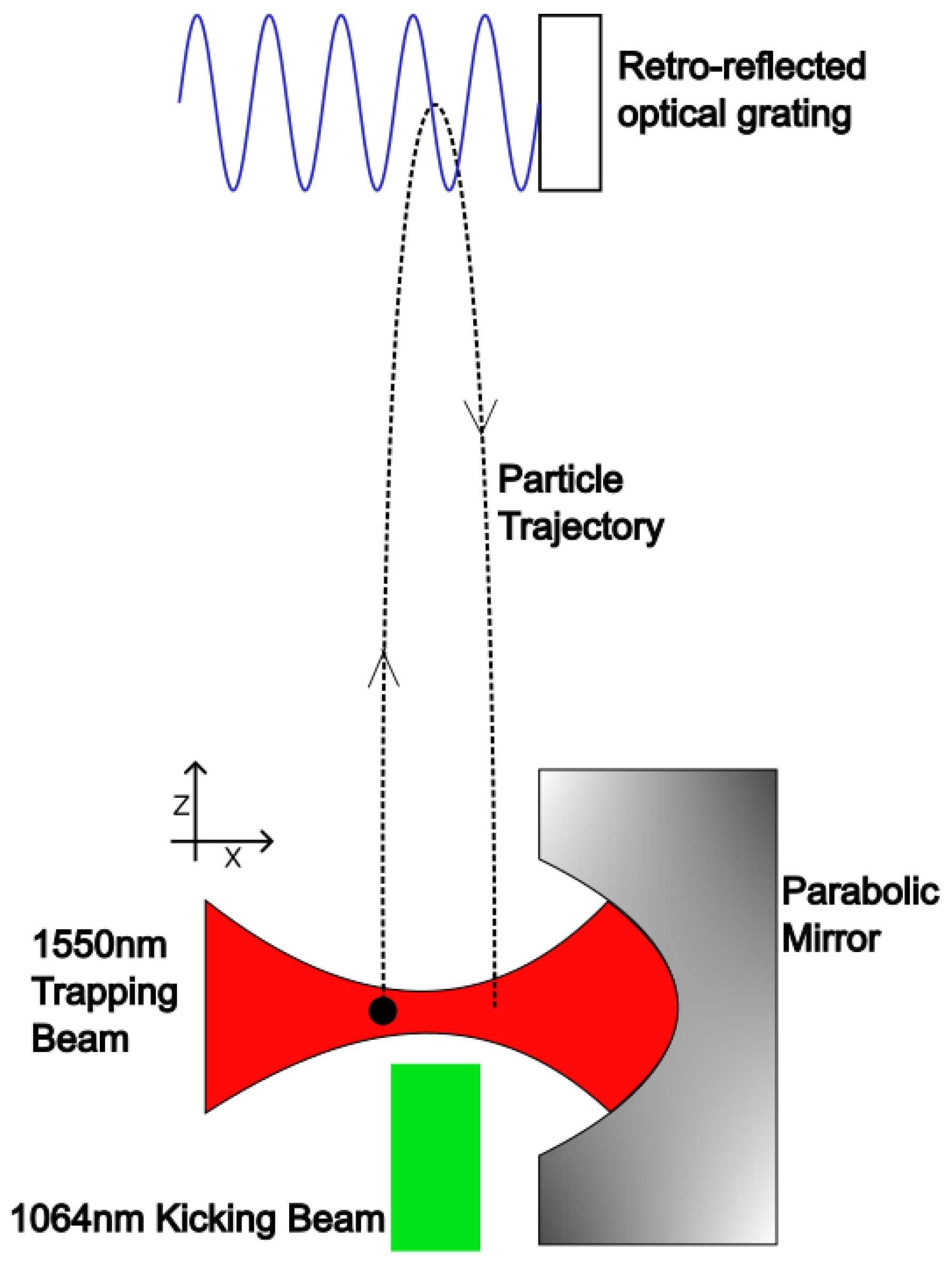
2. Experimental Setup
3. Theoretical Model
3.1. Background
3.2. Accounting for Decoherence and Particle Size
4. Practical Considerations
5. Results
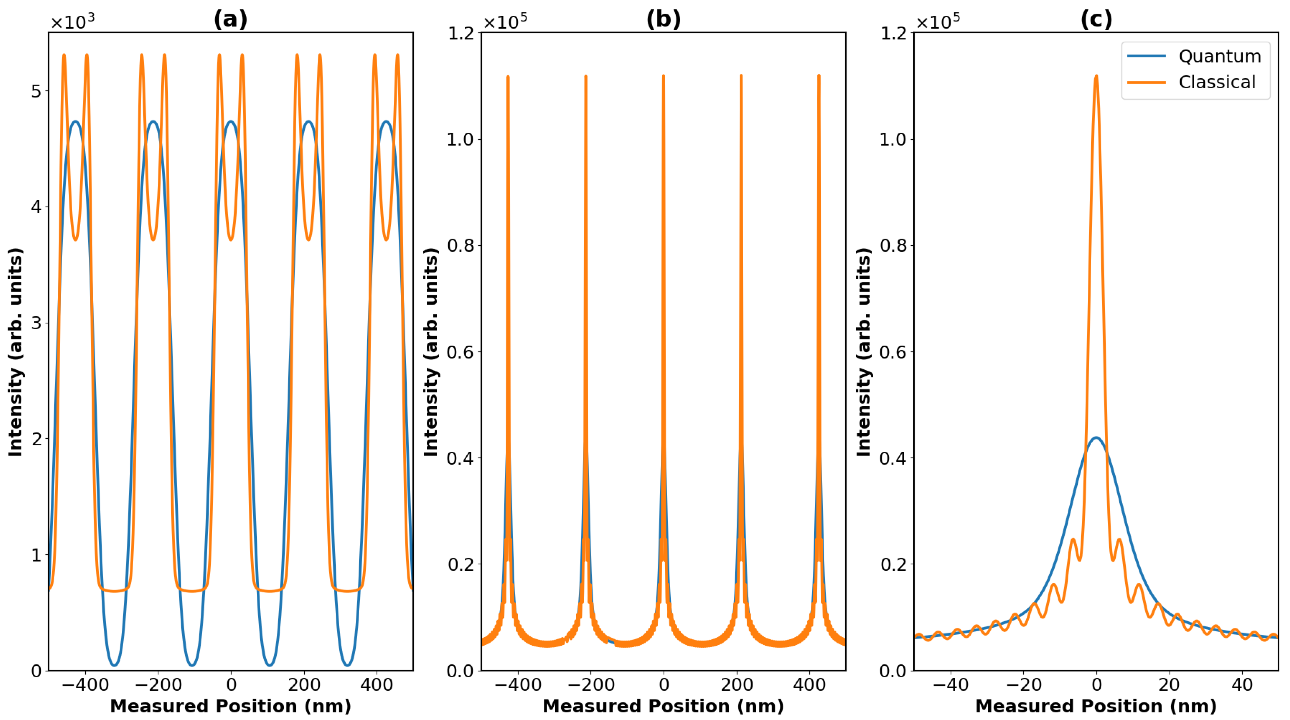
5.1. Expected Interference Patterns
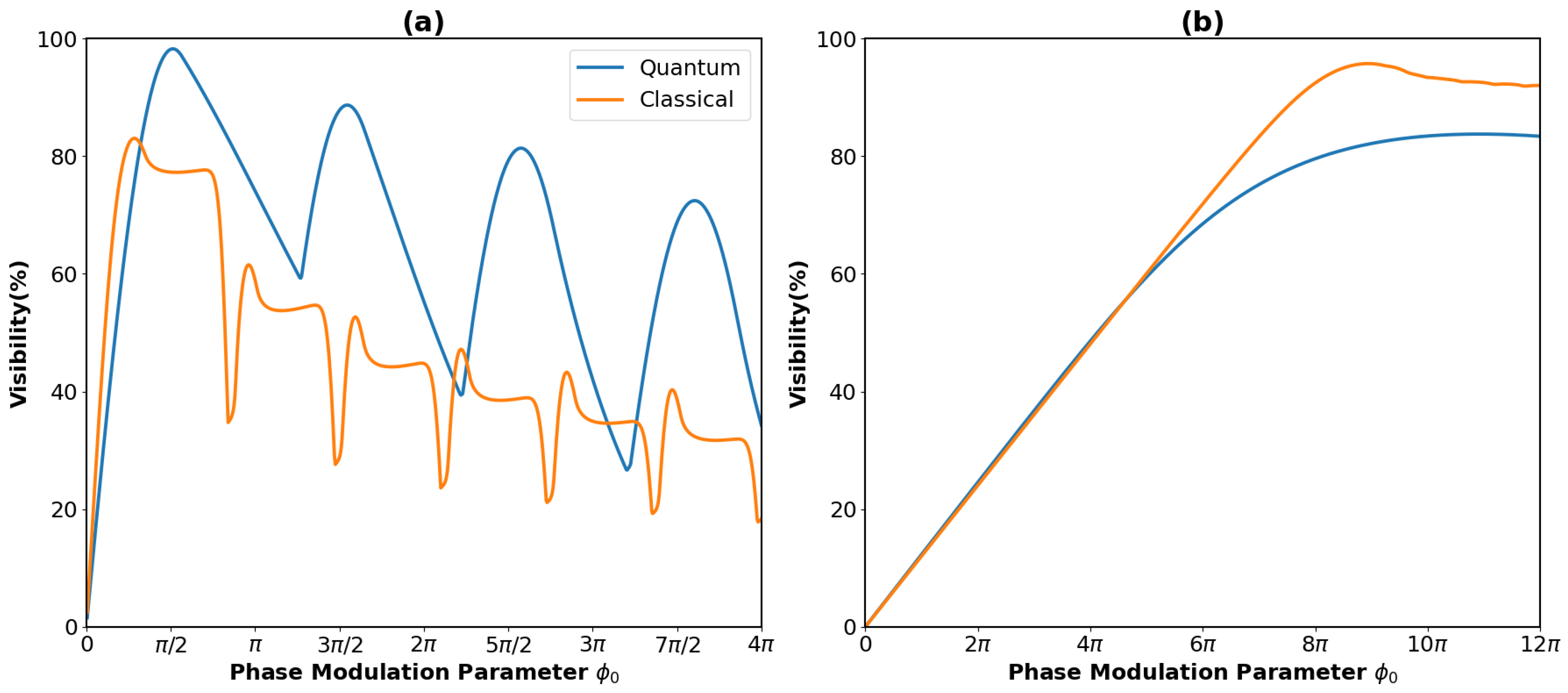
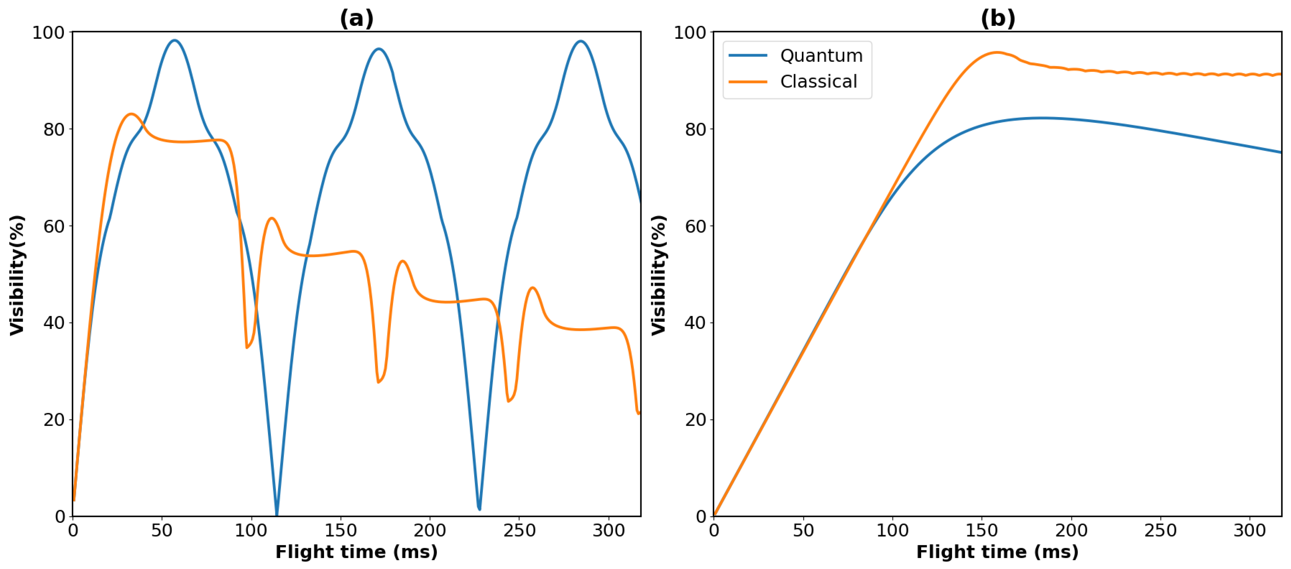
5.2. Quantum/Classical Distinctions
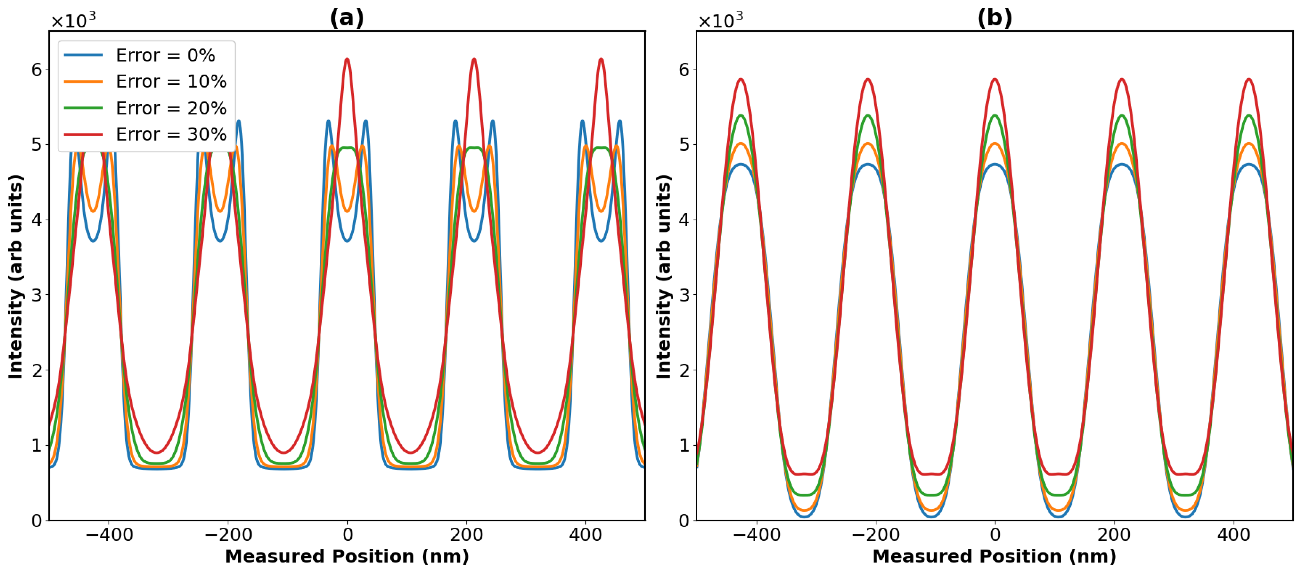
5.3. Throw- and Catch-Specific Decoherence
5.4. Experimental Progress
6. Conclusions
Author Contributions
Funding
Data Availability Statement
Acknowledgments
Conflicts of Interest
Appendix A. Incoherent Sources


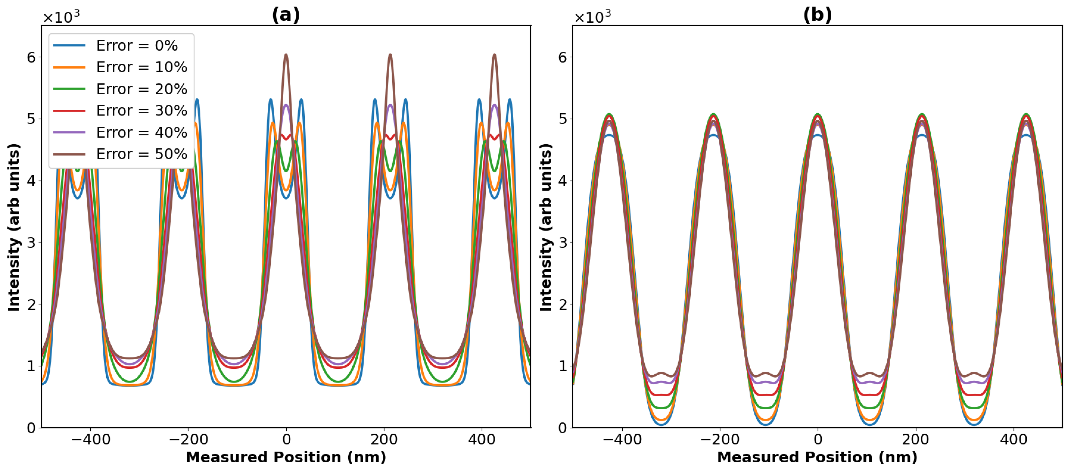
| Mass Error | Classical Fringe Visibility | Quantum Fringe Visibility |
|---|---|---|
| 0% | 77.3% | 98.2% |
| 10% | 75.6% | 95.1% |
| 20% | 72.4% | 88.3% |
| 30% | 66.0% | 81.1% |
| 40% | 67.1% | 74.5% |
| 50% | 68.7% | 71.4% |
Appendix B. Mie Scattering Correction
| 1 | Interference effects between the coherent part of the wave function can only occur if the size of the original source is smaller than the grating period . One furthermore needs , to ensure that the initial trapped state extends over many grating momenta, a necessary condition to guarantee the validity of the theoretical model used to describe the interferometric setup [21,23]. Both of these conditions are fulfilled for the case of study presented here. |
| 2 | |
| 3 | For the case of finite-size particles, we refer the reader to the derivation in [25]. |
| 4 | This is true for a particle optically levitated in vacuum. If the refractive index of the medium is greater than that of the particle, then the particle is pushed away from the maximum field strength region. |
| 5 | Despite the cooling requirements detailed in the previous section, we chose a 1 mK temperature here to demonstrate the relatively low cooling requirements needed to see visible fringes. In theory, should a better solution for recapture be found, this would be the new cooling requirement. Using the temperatures from the previous section would lead to slightly higher visibility fringes. |
References
- Young, T.I. The Bakerian Lecture. Experiments and calculations relative to physical optics. Philos. Trans. R. Soc. Lond. 1804, 94, 1–16. [Google Scholar]
- de Broglie, L. Research on the theory of quanta. Ann. Phys. 1925, 10, 22–128. [Google Scholar] [CrossRef]
- Davisson, C.J.; Germer, L.H. Reflection and Refraction of Electrons by a Crystal of Nickel. Proc. Natl. Acad. Sci. USA 1928, 14, 619–627. [Google Scholar] [CrossRef]
- Zurek, W.H. Decoherence, einselection, and the quantum origins of the classical. Rev. Mod. Phys. 2003, 75, 715–775. [Google Scholar] [CrossRef]
- Schlosshauer, M. Decoherence, the measurement problem, and interpretations of quantum mechanics. Rev. Mod. Phys. 2005, 76, 1267–1305. [Google Scholar] [CrossRef]
- Bose, S.; Mazumdar, A.; Morley, G.W.; Ulbricht, H.; Toroš, M.; Paternostro, M.; Geraci, A.A.; Barker, P.F.; Kim, M.S.; Milburn, G. Spin Entanglement Witness for Quantum Gravity. Phys. Rev. Lett. 2017, 119, 240401. [Google Scholar] [CrossRef]
- Marletto, C.; Vedral, V. Gravitationally Induced Entanglement between Two Massive Particles is Sufficient Evidence of Quantum Effects in Gravity. Phys. Rev. Lett. 2017, 119, 240402. [Google Scholar] [CrossRef] [PubMed]
- Estermann, I.; Stern, O. Beugung von Molekularstrahlen. Z. Phys. 1930, 61, 95–125. [Google Scholar] [CrossRef]
- Gould, P.L.; Ruff, G.A.; Pritchard, D.E. Diffraction of atoms by light: The near-resonant Kapitza-Dirac effect. Phys. Rev. Lett. 1986, 56, 827. [Google Scholar] [CrossRef] [PubMed]
- Keith, D.; Schattenburg, M.; Smith, H.I.; Pritchard, D. Diffraction of atoms by a transmission grating. Phys. Rev. Lett. 1988, 61, 1580. [Google Scholar] [CrossRef] [PubMed]
- Bordé, C.J. Atomic interferometry with internal state labelling. Phys. Lett. A 1989, 140, 10–12. [Google Scholar] [CrossRef]
- Kasevich, M.; Chu, S. Atomic interferometry using stimulated Raman transitions. Phys. Rev. Lett. 1991, 67, 181. [Google Scholar] [CrossRef] [PubMed]
- Hornberger, K.; Gerlich, S.; Haslinger, P.; Nimmrichter, S.; Arndt, M. Colloquium: Quantum interference of clusters and molecules. Rev. Mod. Phys. 2012, 84, 157. [Google Scholar] [CrossRef]
- Fein, Y.Y.; Geyer, P.; Zwick, P.; Kiałka, F.; Pedalino, S.; Mayor, M.; Gerlich, S.; Arndt, M. Quantum superposition of molecules beyond 25 kDa. Nat. Phys. 2019, 15, 1242–1245. [Google Scholar] [CrossRef]
- Clauser, J.F.; Li, S. Generalized Talbot–Lau Atom Interferometry. In Atom Interferometry; Berman, P.R., Ed.; Academic Press: San Diego, CA, USA, 1997; pp. 121–151. [Google Scholar]
- Arndt, M.; Nairz, O.; Voss-Andreae, J.; Keller, C.; Zouw, G.; Zeilinger, A. Wave-particle duality of C60 molecules. Nature 1999, 401, 680–682. [Google Scholar] [CrossRef]
- Brezger, B.; Hackermüller, L.; Uttenthaler, S.; Petschinka, J.; Arndt, M.; Zeilinger, A. Matter wave interferometer for large molecules. Phys. Rev. Lett. 2002, 88, 100404. [Google Scholar] [CrossRef] [PubMed]
- Arndt, M.; Hornberger, K. Testing the limits of quantum mechanical superpositions. Nat. Phys. 2014, 10, 271–277. [Google Scholar] [CrossRef]
- Juffmann, T.; Ulbricht, H.; Arndt, M. Experimental methods of molecular matter wave optics. Rep. Prog. Phys. 2013, 76, 086402. [Google Scholar] [CrossRef]
- Gonzalez-Ballestero, C.; Aspelmeyer, M.; Novotny, L.; Quidant, R.; Romero-Isart, O. Levitodynamics: Levitation and control of microscopic objects in vacuum. Science 2021, 374, eabg3027. [Google Scholar] [CrossRef]
- Bateman, J.; Nimmrichter, S.; Hornberger, K.; Ulbricht, H. Near-field interferometry of a free-falling nanoparticle from a point-like source. Nat. Commun. 2014, 5, 4788. [Google Scholar] [CrossRef]
- Vovrosh, J.; Rashid, M.; Hempston, D.; Bateman, J.; Paternostro, M.; Ulbricht, H. Parametric feedback cooling of levitated optomechanics in a parabolic mirror trap. JOSA B 2017, 34, 1421–1428. [Google Scholar] [CrossRef]
- Nimmrichter, S.; Hornberger, K. Theory of near-field matter wave interference beyond the eikonal approximation. Phys. Rev. A 2008, 78, 023612. [Google Scholar] [CrossRef]
- Hebestreit, E.; Frimmer, M.; Reimann, R.; Novotny, L. Sensing Static Forces with Free-Falling Nanoparticles. Phys. Rev. Lett. 2018, 121, 063602. [Google Scholar] [CrossRef] [PubMed]
- Belenchia, A.; Gasbarri, G.; Kaltenbaek, R.; Ulbricht, H.; Paternostro, M. Talbot–Lau effect beyond the point-particle approximation. Phys. Rev. A 2019, 100. [Google Scholar] [CrossRef]
- Nimmrichter, S. Macroscopic Matter Wave Interferometry; Springer: Berlin/Heidelberg, Germany, 2014. [Google Scholar]
- Laing, S.; Bateman, J. Bayesian inference for near-field interferometric tests of collapse models. arXiv 2023, arXiv:2310.05763. [Google Scholar]
- Hebestreit, E. Thermal Properties of Levitated Nanoparticles. Ph.D. Thesis, ETH Zurich, Zurich, Switzerland, 2017. [Google Scholar]
- Delić, U.; Reisenbauer, M.; Dare, K.; Grass, D.; Vuletić, V.; Kiesel, N.; Aspelmeyer, M. Cooling of a levitated nanoparticle to the motional quantum ground state. Science 2020, 367, 892–895. [Google Scholar] [CrossRef]
- Rohrbach, A.; Stelzer, E.H. Optical trapping of dielectric particles in arbitrary fields. JOSA A 2001, 18, 839–853. [Google Scholar] [CrossRef]
- Ransom, M.J.; Vladimirov, L.; Horridge, P.R.; Ralph, J.F.; Maskell, S. Integrated Expected Likelihood Particle Filters. In Proceedings of the 2020 IEEE 23rd International Conference on Information Fusion (FUSION), Rustenburg, South Africa, 6–9 July 2020; pp. 1–8. [Google Scholar]


| Parameter | amu Particle | amu Particle |
|---|---|---|
| Pressure | mbar | mbar |
| Initial temperature | 1 mK | 1 mK |
| Flight time | 58 ms | 142 ms |
| Phase modulation () |
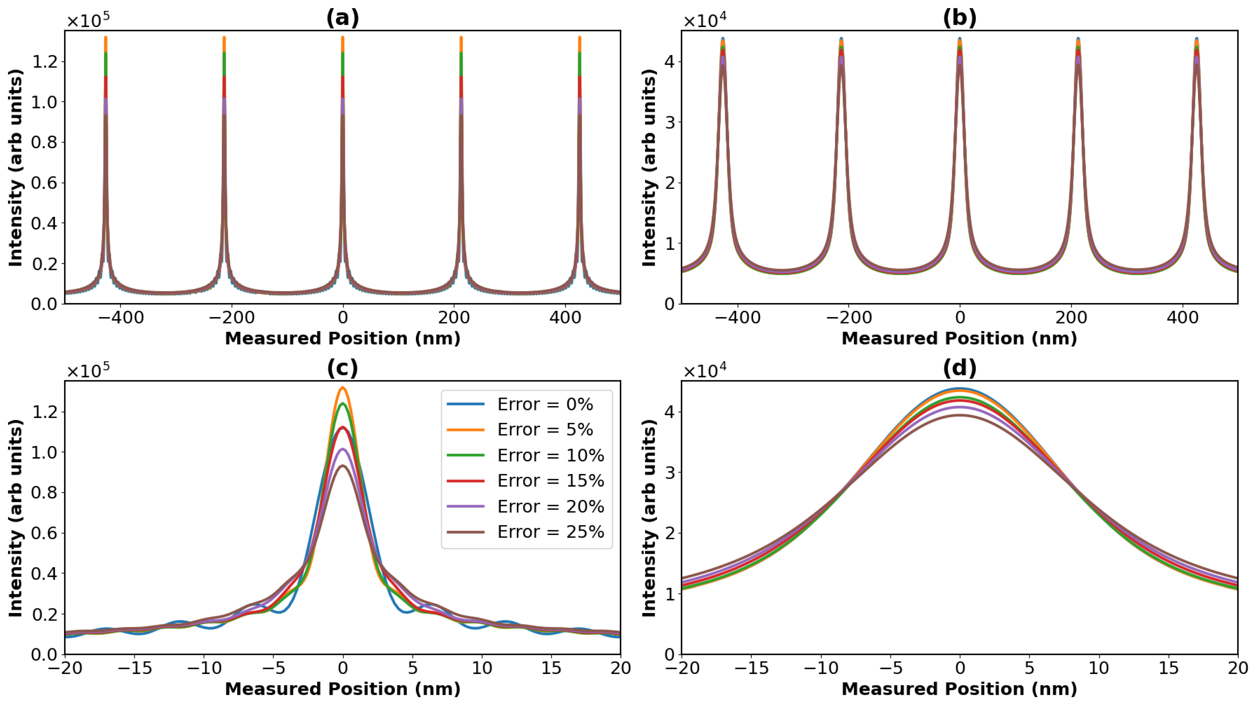
| Velocity Error | Classical Fringe Visibility | Quantum Fringe Visibility |
|---|---|---|
| 0% | 77.3% | 98.2% |
| 10% | 75.0% | 94.9% |
| 20% | 73.5% | 88.3% |
| 30% | 74.5% | 81.1% |
| Velocity Error | Classical Fringe Visibility | Quantum Fringe Visibility |
|---|---|---|
| 0% | 92.2% | 79.6% |
| 5% | 93.0% | 79.6% |
| 10% | 92.5% | 79.1% |
| 15% | 91.5% | 78.4% |
| 20% | 90.3% | 77.2% |
| 25% | 89.0% | 75.5% |
Disclaimer/Publisher’s Note: The statements, opinions and data contained in all publications are solely those of the individual author(s) and contributor(s) and not of MDPI and/or the editor(s). MDPI and/or the editor(s) disclaim responsibility for any injury to people or property resulting from any ideas, methods, instructions or products referred to in the content. |
© 2024 by the authors. Licensee MDPI, Basel, Switzerland. This article is an open access article distributed under the terms and conditions of the Creative Commons Attribution (CC BY) license (https://creativecommons.org/licenses/by/4.0/).
Share and Cite
Wardak, J.; Georgescu, T.; Gasbarri, G.; Belenchia, A.; Ulbricht, H. Nanoparticle Interferometer by Throw and Catch. Atoms 2024, 12, 7. https://doi.org/10.3390/atoms12020007
Wardak J, Georgescu T, Gasbarri G, Belenchia A, Ulbricht H. Nanoparticle Interferometer by Throw and Catch. Atoms. 2024; 12(2):7. https://doi.org/10.3390/atoms12020007
Chicago/Turabian StyleWardak, Jakub, Tiberius Georgescu, Giulio Gasbarri, Alessio Belenchia, and Hendrik Ulbricht. 2024. "Nanoparticle Interferometer by Throw and Catch" Atoms 12, no. 2: 7. https://doi.org/10.3390/atoms12020007