Variational Approaches to Two-Dimensionally Symmetry-Broken Dipolar Bose–Einstein Condensates

Abstract

It has been shown that quantum fluctuations in dipolar Bose–Einstein condensates (BECs) lead to a stabilisation against collapse, thereby providing access to a range of states with different symmetries. In this paper, we discuss variational approaches to approximately determine the phase diagrams for dipolar BECs that are trapped along the dipolar orientation and otherwise infinite in the perpendicular direction (thermodynamic limit). The two-dimensional symmetry breaking occurs in the plane perpendicular to the polarisation axis. We show in detail how to derive approximate expressions that are valid in a region where modulations to an otherwise unmodulated perfect superfluid emerge gradually with a small modulation amplitude and compare the results to rigorous numerics.

1. Introduction

The formation of self-organised structures is captivating to natural scientists from a broad range of subjects [1,2,3]. A curious phenomenon was conceived roughly fifty years [4,5,6] ago related to patterned solid-like distributions of the quantum wave function: It was conjectured that—despite displaying a regular spatial discrete translational symmetry akin to a solid with which we intuitively associate rigidity or resistance to shear—the superfluid fraction can remain significant. Therefore, this idea was coined as a superfluid crystal or “supersolid”.

A range of interesting physical phenomena are possible in Bose–Einstein condensates (BECs) exhibiting long-range interactions, including the formation of self-trapped droplets [7,8,9,10,11,12] or collective excitations [13,14,15,16,17] akin to superfluid helium [18]. In particular, BECs with strong dipolar interactions turned out to be a remarkable setting, thus permitting the realisation of a range of experimental breakthroughs [19,20,21,22,23,24,25,26,27,28,29,30,31,32]. Amongst the reasons as to why the experiments on dipolar BECs carry such significance is the fact that, instead of exhibiting a collapsing wave function [33,34] as expected from the mean-field theory, there is a significant stabilisation mechanism [35,36,37,38,39,40] at play that is due to (beyond mean-field) quantum-fluctuations [41,42]. Hence, the macroscopically visible mere existence of non-collapsing density distributions reveals information about the underlying microscopic beyond-mean field behaviour that is otherwise hard to access.

Due to the suppression of collapse, the characteristic roton softening of the dipolar interaction [13] becomes accessible, thereby providing a platform that permits the exploration of a range of features of the earlier-mentioned supersolid. These include the measurement of the superfluid–supersolid phase transition [26,27,28], supersolid excitation spectra [29,30], and transient behaviour [24,25], as well as the probing of nonclassical rotational inertia [31] and their temperature dependence [32,43].

Beyond its stabilising effect against collapse, quantum fluctuations have been predicted to also alter the phase diagram of BECs with two-dimensionally symmetry-broken states. Furthermore, it has been shown that the latter gives rise to new phases of matter [44,45,46,47], which display different supersolid properties [48] and a point in the phase diagram where the superfluid–supersolid phase transition becomes of second-order, rather than the first-order phase transition otherwise expected for such states [44]. Whereas they are experimentally challenging to create, there are already efforts towards realising two-dimensional supersolids [49,50,51,52].

The numerical simulation of these systems is computationally expensive; therefore, it is desirable to employ approximate variational techniques to identify interesting parameter regions, as well as to obtain a qualitative understanding of the underlying physics. Such variational techniques have been employed in [44,45]; however, a detailed derivation, as well as a discussion of its suitability, have not yet been provided thus far. In this paper, we would like to present the latter. In particular, we present a small amplitude expansion that permits a qualitative understanding of the phase diagram and, furthermore, yields some quantitatively reasonably correct results such as the location of the second-order point.

In Section 2, we provide the model employed to describe the dipolar Bose–Einstein condensate that displays appreciable quantum fluctuations. Section 3 presents a derivation of the expansion of the energy shift to fourth order in modulation amplitude and a subsequent single-mode approximation. After that, a comparison between infinite order and fourth order in amplitude, as well as full numerical results, are provided. In Section 5, we conclude.

2. Theoretical Model

We consider a zero-temperature quantum gas of N dipolar Bosonic atoms with mass m that are harmonically trapped along the dipolar polarization axis z. In order to be able to use variational approaches and to simplify the discussion, it is useful to consider a system that is unconfined in the $(x,y)$ plane perpendicular to the polarization axis. The particles composing the BEC interact via s-wave scattering with scattering length $a_{\mathrm{s}}$ and via an anisotropic long-range interaction between the atomic dipoles characterised by an associated length scale $a_{\mathrm{dd}}$ [53].

We use the convention that the wave function $\psi (\mathbf{r},t)$ of the atoms is normalised to the total particle number N, i.e., ${\int \left|\psi \right|}^2{\mathrm{d}}^{3}r=N$, and $\rho ={\left|\psi \right|}^2$ corresponds to the atomic density. We use scaled variables to simplify the discussion and express spatial coordinates in units of $\ell =12\pi a_{\mathrm{dd}}$ and time in units of $\tau =m{\ell }^2/\hslash$. With that, we can write the total energy E of the Bose–Einstein condensate as follows:

$$\begin{array}{cc}\hfill E& =\int \left(\frac{{|\nabla \psi \left(\mathbf{r}\right)|}^2}{2}+{U\left(z\right)\left|\psi \left(\mathbf{r}\right)\right|}^2+\frac{a_{\mathrm{s}}}{6a_{\mathrm{dd}}}{\left|\psi \left(\mathbf{r}\right)\right|}^4+\frac{2}{5}\gamma {\left|\psi \left(\mathbf{r}\right)\right|}^5\right){\mathrm{d}}^{3}r\hfill \\ \hfill & +\int \frac{{\left|\psi \left(\mathbf{r}\right)\right|}^2}{8\pi }\int V(\mathbf{r}-{\mathbf{r}}^{\prime }){\left|\psi \left({\mathbf{r}}^{\prime }\right)\right|}^2{\mathrm{d}}^3{r}^{\prime }{\mathrm{d}}^{3}r.\hfill \end{array}$$

(1)

The first and second term describe the single-particle contributions corresponding to the kinetic energy of the atoms and the energy due to the trapping potential $U\left(z\right)=\frac{1}{2}{\omega }_z^2{z}^2$, respectively. The third term describes the zero-range scattering interaction between the atoms, and the fourth contribution is the so-called Lee–Huang–Yang [54,55] correction describing quantum fluctuations to leading order in the strength of the atomic interactions. Here, we have introduced $\gamma =\frac{4}{3{\pi }^2}{\left(\frac{a_{\mathrm{s}}}{3a_{\mathrm{dd}}}\right)}^{5/2}[1+\frac{3}{2}{\left(\frac{a_{\mathrm{dd}}}{a_{\mathrm{s}}}\right)}^2]$ [35,36,41,42] to denote the strength of the quantum fluctuations. The fifth term is due to long-ranged dipolar interatomic interactions. We assume that the magnetic dipoles are aligned along the trapping direction z.

3. Variational Ansatz

It has already been shown that there is a special point [44] in the phase diagram in this system. Sufficiently close to this point, states with broken continuous translational symmetry with near-perfect superfluidity emerge gradually with arbitrarily small amplitudes on an otherwise unmodulated background, which is characteristic for a second-order phase-transition. In the following, we will simply refer to this point as a second-order point.

When sufficiently close to that point, it is reasonable to employ a small-amplitude approximation. This will be presented in Section 3.1. After that, we will use different single-mode approximations to describe the following symmetries: triangular or honeycomb lattices, stripe, and square lattices.

3.1. Small-Amplitude Expansion

In this subsection, we present a small-amplitude expansion that is valid close to the second-order point. This details and complements the results presented in [44,45]. More specifically, we consider a small-amplitude expansion of the energy-shift to the fourth order. This is the lowest possible order of expansion that permits understanding the essential physics of symmetry breaking: We will find that large amplitudes are suppressed (or rendered energetically unfavorably) by the fourth-order contribution, the second-order contribution in amplitude drives the transition for suitable parameters, and the third-order term leads to different symmetry-breaking scenarios, in that it determines whether the phase transition is of the first- or second-order and it leads to the formation of different lattice types. It is convenient to employ the Madelung transform and express the wave function as $\psi \left(\mathbf{r}\right)=\sqrt{\rho \left(\mathbf{r}\right)}{e}^{i\varphi }$. That permits rewriting the energy Equation (1) as follows:

$$\begin{array}{cc}\hfill E=& \int [-\frac{1}{2}{\psi }^{*}{\nabla }^2\psi +\frac{1}{2}{\omega }_z^2{z}^2{\left|\psi \right|}^2+\frac{a_s}{6a_{\mathrm{dd}}}{\left|\psi \right|}^4+\frac{2}{5}\gamma {\left|\psi \right|}^5\hfill \\ \hfill & +\frac{1}{8\pi }\int U_{\mathrm{dd}}(\mathbf{r}-{\mathbf{r}}^{\prime })|\psi \left({\mathbf{r}}^{\prime }\right){|}^2{\left|\psi \left(\mathbf{r}\right)\right|}^2{d}^3{r}^{\prime }]d^{3}r\hfill \\ \hfill =& \int [\frac{{(\nabla \rho )}^2}{8\rho }-\frac{{\nabla }^2\rho }{4}+\frac{1}{2}{\omega }_z^2{z}^2\rho +\frac{a_s}{6a_{\mathrm{dd}}}{\rho }^2+\frac{2}{5}\gamma {\rho }^{5/2}\hfill \\ \hfill & +\frac{1}{8\pi }\int U_{\mathrm{dd}}(\mathbf{r}-{\mathbf{r}}^{\prime })\rho \left({\mathbf{r}}^{\prime }\right)\rho \left(\mathbf{r}\right)d^3{r}^{\prime }]d^{3}r.\hfill \end{array}$$

(2)

Let ${\rho }_0$ denote the density of the ground state. In the following, we want to explore how small perturbations $\delta \rho$ to this state manifest as a shift $\delta E$ to the energy. The latter can be expressed as follows:

$$\begin{array}{cc}\hfill \delta E=& E({\rho }_0+\delta \rho )-E\left({\rho }_0\right)\hfill \\ \hfill =& \int \left[\frac{{(\nabla {\rho }_0+\nabla \delta \rho )}^2}{8({\rho }_0+\delta \rho )}-\frac{{\rho }_0+\delta \rho }{8{\rho }_0^2}{(\nabla {\rho }_0)}^2+\frac{\delta \rho {\nabla }^2{\rho }_0-{\rho }_0{\nabla }^2\delta \rho }{4{\rho }_0}\right]d^{3}r+\int {\mu }_0\delta \rho d^{3}r\hfill \\ \hfill & +\int [\frac{a_s}{6a_{\mathrm{dd}}}\delta {\rho }^2+\frac{2}{5}\gamma \left(\frac{15}{8}\sqrt{{\rho }_0}\delta {\rho }^2+\frac{5}{16}\frac{\delta {\rho }^3}{\sqrt{{\rho }_0}}-\frac{5}{128}\frac{\delta {\rho }^4}{{\rho }_0^{3/2}}+\cdots \right)\hfill \\ \hfill & +\frac{1}{8\pi }\delta \rho \left(\mathbf{r}\right)\int U_{\mathrm{dd}}(\mathbf{r}-{\mathbf{r}}^{\prime })\delta \rho \left({\mathbf{r}}^{\prime }\right)d^3{r}^{\prime }]d^{3}r.\hfill \end{array}$$

Here, we introduce the chemical potential of the non-perturbed state as follows:

$$\begin{array}{cc}\hfill {\mu }_0=& -\frac{\partial \varphi }{\partial t}=\frac{{(\nabla {\rho }_0)}^2}{8{\rho }_0^2}-\frac{{\nabla }^2{\rho }_0}{4{\rho }_0}+\frac{1}{2}{\omega }_z^2{z}^2+\frac{a_s}{3a_{\mathrm{dd}}}{\rho }_0+\gamma {\rho }_0^{3/2}+\frac{1}{4\pi }\int U_{\mathrm{dd}}(\mathbf{r}-{\mathbf{r}}^{\prime }){\rho }_0\left({\mathbf{r}}^{\prime }\right)d^3{r}^{\prime }.\hfill \end{array}$$

We restrict our considerations to situations where the total particle number is conserved. Therefore, the possible perturbations are constrained by $\int \delta \rho d^{3}r=0$. This constraint gives rise to the following:

$$\begin{array}{cc}\hfill \delta E& =\int [\frac{{(\nabla {\rho }_0)}^2}{8{\rho }_0}\left(-\frac{2\delta \rho }{{\rho }_0}+{\left(\frac{\delta \rho }{{\rho }_0}\right)}^2-{\left(\frac{\delta \rho }{{\rho }_0}\right)}^3+{\left(\frac{\delta \rho }{{\rho }_0}\right)}^4+\cdots \right)\hfill \\ \hfill & +\frac{2\nabla {\rho }_0·\nabla \delta \rho +{(\nabla \delta \rho )}^2}{8{\rho }_0}\left(1-\frac{\delta \rho }{{\rho }_0}+{\left(\frac{\delta \rho }{{\rho }_0}\right)}^2-{\left(\frac{\delta \rho }{{\rho }_0}\right)}^3+{\left(\frac{\delta \rho }{{\rho }_0}\right)}^4+\cdots \right)+\hfill \\ \hfill & \frac{\delta \rho {\nabla }^2{\rho }_0-{\rho }_0{\nabla }^2\delta \rho }{4{\rho }_0}]d^{3}r+\int [\frac{a_s}{6a_{\mathrm{dd}}}\delta {\rho }^2+\frac{2}{5}\gamma \left(\frac{15}{8}\sqrt{{\rho }_0}\delta {\rho }^2+\frac{5}{16}\frac{\delta {\rho }^3}{\sqrt{{\rho }_0}}-\frac{5}{128}\frac{\delta {\rho }^4}{{\rho }_0^{3/2}}+\cdots \right)\hfill \\ \hfill & +\frac{1}{8\pi }\delta \rho \left(\mathbf{r}\right)\int U_{\mathrm{dd}}(\mathbf{r}-{\mathbf{r}}^{\prime })\delta \rho \left({\mathbf{r}}^{\prime }\right)d^3{r}^{\prime }]d^{3}r.\hfill \end{array}$$

As there is only confinement in the polarization direction z, the unmodulated state ${\rho }_0$ only depends on z; therefore, ${\rho }_0\left(\mathbf{r}\right)={\rho }_0\left(z\right)$. Since the dipole–dipole interaction is anisotropic (i.e., attractive along the polarization direction z and repulsive in the transverse direction), the roton instability (crystallization) of the dipolar BEC can occur in the transverse plane only. As ansatz for the full density $\rho ={\rho }_0+\delta \rho$, including the perturbation $\delta \rho$ occurring in the transverse unconfined plane, it is reasonable to assume the form

$$\delta \rho ={\rho }_0\left(z\right)P(x,y)$$

(3)

if the amplitude of P is sufficiently small and the error of the factorisation remains small. In other words, we assume that P is a periodic function containing two variational parameters, the periodicity in the transverse plane $k_{\perp }=2\pi /\lambda$, and its amplitude A. Given that the equation of motion is nonlinear and even contains a three-dimensional convolution, it is not at all evident that such a factorisation holds for a certain parameter region. However, if the amplitude of P remains sufficiently small, such that the main spatial variation is already captured by ${\rho }_0$, the error of the factorisation remains small, since we can undertake an expansion in the small amplitude of P. In that sense, P has both the character of a variational and a perturbative function.

With this ansatz, we can find the following expression for $\delta E$:

$$\begin{array}{cc}\hfill \delta E& =\frac{1}{8}{\int }_{-\infty }^{+\infty }{\rho }_0\left(z\right)dz{\int }_0^{L_x}{\int }_0^{L_y}\left[{\left(\frac{\partial P}{\partial x}\right)}^2+{\left(\frac{\partial P}{\partial y}\right)}^2\right]\left(1-P+P^2-P^3+P^4+\cdots \right)dxdy\hfill \\ \hfill & +\frac{a_s}{6a_{\mathrm{dd}}}{\int }_{-\infty }^{+\infty }{\rho }_0^2\left(z\right)dz{\int }_0^{L_x}{\int }_0^{L_y}{P}^{2}dxdy\hfill \\ \hfill & +\gamma {\int }_{-\infty }^{+\infty }{\rho }_0^{5/2}\left(z\right)dz{\int }_0^{L_x}{\int }_0^{L_y}\left(\frac{3}{4}{P}^2+\frac{1}{8}{P}^3-\frac{1}{64}{P}^4+\cdots \right)dxdy\hfill \\ \hfill & +\frac{1}{2}\int {\rho }_0\left(z\right)P(x,y)\frac{1}{{\left(2\pi \right)}^{3/2}}\int \left(\frac{k_z^2}{k_z^2+k_{\perp }^2}-\frac{1}{3}\right){\rho }_0\left(k_z\right)P\left(k_{\perp }\right)e^{i\mathbf{k}·\mathbf{r}}{d}^{3}k{d}^{3}r.\hfill \end{array}$$

(4)

Here, we use the analytical expression for the Fourier transform of the dipolar interaction. The convention for the Fourier transform we employ is as follows:

$$\begin{array}{c}\hfill f\left(\mathbf{k}\right)=\frac{1}{{\left(2\pi \right)}^{3/2}}\int f\left(\mathbf{r}\right)e^{-i\mathbf{k}·\mathbf{r}}{d}^{3}r.\end{array}$$

(5)

Therefore, ${\rho }_0\left(k_z\right)=\frac{1}{\sqrt{2\pi }}\int {\rho }_0\left(z\right)e^{-i{k}_{z}z}dz$, and $P\left(k_{\perp }\right)=\frac{1}{2\pi }\int P(x,y)e^{-i{\mathbf{k}}_{\perp }·{\mathbf{r}}_{\perp }}{d}^2{r}_{\perp }$. Here, we introduced the transverse coordinates ${\mathbf{r}}_{\perp }=(x,y)$ and ${\mathbf{k}}_{\perp }=(k_x,k_y)$, respectively.

As an approximation for ${\rho }_0\left(z\right)$, we assume a Thomas–Fermi profile:

$${\rho }_0\left(z\right)=\frac{3n_{2\mathrm{D}}}{4{\sigma }_z}\left(1-\frac{z^2}{{\sigma }_z^2}\right).$$

(6)

Here, we introduce the auxiliary two-dimensional density $n_{2\mathrm{D}}=N/\mathcal{A}$ as the ratio between total particle number N and the transverse area $\mathcal{A}$. Both N and $\mathcal{A}$ diverge in the thermodynamic limit, but $n_{2\mathrm{D}}$ remains finite and well-defined. The amplitude of ${\rho }_0\left(z\right)$ is chosen in such a way that ${\int }_{-{\sigma }_z}^{{\sigma }_z}{\rho }_0\left(z\right)\mathrm{d}z=n_{2\mathrm{D}}$.

With the Thomas–Fermi profile for ${\rho }_0\left(z\right)$, we are now in a position to evaluate the chemical potential ${\mu }_0$ of the unmodulated state. As for the derivation of the Thomas–Fermi profile it is generally assumed that the kinetic energy is zero, we neglect the kinetic contribution to ${\mu }_0$ as well. Furthermore, we assume that one can neglect the Lee–Huang–Yang correction for this consideration. With that, we find the following:

$$\begin{array}{cc}\hfill {\mu }_0& =\frac{1}{2}{\omega }_z^2{z}^2+\frac{a_s}{3a_{\mathrm{dd}}}{\rho }_0+\frac{1}{4\pi }\int U_{\mathrm{dd}}(\mathbf{r}-{\mathbf{r}}^{\prime }){\rho }_0\left({\mathbf{r}}^{\prime }\right)d^3{r}^{\prime }\hfill \\ \hfill & =\frac{1}{2}{\omega }_z^2{z}^2+\frac{a_s}{3a_{\mathrm{dd}}}{\rho }_0\left(z\right)+\frac{1}{2\pi }\int \frac{2}{3}\int {\rho }_0\left(z^{\prime }\right)e^{i{k}_z{z}^{\prime }}d{z}^{\prime }{e}^{-i{k}_{z}z}d{k}_z\hfill \\ \hfill & =\frac{1}{2}{\omega }_z^2{z}^2+\frac{a_s}{3a_{\mathrm{dd}}}{\rho }_0\left(z\right)+\int \frac{2}{3}{\rho }_0\left(z^{\prime }\right)\delta (z-z^{\prime })d{z}^{\prime }\hfill \\ \hfill & =\frac{1}{2}{\omega }_z^2{z}^2+\frac{a_s}{3a_{\mathrm{dd}}}{\rho }_0\left(z\right)+\frac{2}{3}{\rho }_0\left(z\right).\hfill \end{array}$$

The last equation can be solved for ${\rho }_0\left(z\right)$, which allows us to identify an approximate width ${\sigma }_z$ via

$${\rho }_0\left(z\right)=\frac{{\mu }_0}{\frac{a_{\mathrm{s}}}{3a_{\mathrm{dd}}}+\frac{2}{3}}\left(1-\frac{\frac{1}{2}{\omega }_z^2}{{\mu }_0}{z}^2\right).$$

(7)

By comparing the amplitude and width of Equation (7) with (6), one can readily obtain the chemical potential ${\mu }_0$ and the width ${\sigma }_z$ of the Thomas–Fermi profile as

$$\begin{array}{cc}\hfill {\mu }_0& =\frac{n_{2\mathrm{D}}}{4{\sigma }_z}\left(\frac{a_{\mathrm{s}}}{a_{\mathrm{dd}}}+2\right)\hfill \end{array}$$

(8)

$$\begin{array}{cc}\hfill {\sigma }_z& ={\left(\frac{n_{2\mathrm{D}}(a_{\mathrm{s}}/a_{\mathrm{dd}}+2)}{2{\omega }_z^2}\right)}^{1/3}.\hfill \end{array}$$

(9)

We are now in a position where we can evaluate the energy shift due to the periodic perturbation $P(x,y)$. In the following two subsections, we will evaluate the respective expressions for different symmetries.

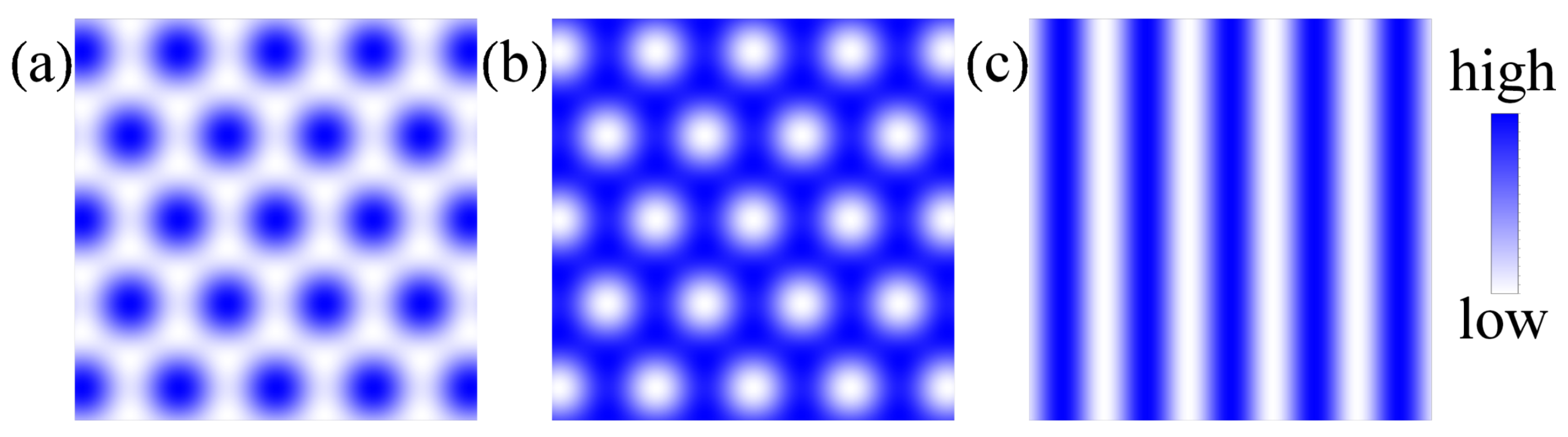
3.2. Hexagonal and Honeycomb Lattices

Thus far, we did not yet specify the symmetry for the periodic perturbation $P(x,y)$. Let us assume that $P(x,y)$ features a triangular symmetry and that further Fourier peaks can be neglected. In that situation, a reasonable ansatz for P is given by

$$P(x,y)=A\sum _{j=1}^{3}cos({\mathbf{k}}_j·{\mathbf{r}}_{\perp }+{\theta }_j),\sum _{j=1}^3{\mathbf{k}}_j=0,$$

(10)

which gives rise to two distinct density distributions depending on the sign of the modulation amplitude A. As shown in Figure 1, the normalized total density $1+P(x,y)$ features a triangular and a honeycomb profile for positive and negative A, respectively.

The most complicated contribution to calculate is the shift in energy due to the dipolar long-range interaction. The other contributions are quite straightforward. Therefore, we will only present the calculation for the dipolar term in detail and state the other cases for the sake of completeness.

$$\begin{array}{cc}\hfill & \Delta E_{\mathrm{ddi}}=\frac{1}{2}\int {\rho }_0\left(z\right)P(x,y)\frac{1}{{\left(2\pi \right)}^{3/2}}\int \left(\frac{k_z^2}{k_z^2+k_{\perp }^2}-\frac{1}{3}\right){\rho }_0\left(k_z\right)P\left(k_{\perp }\right)e^{i\mathbf{k}·\mathbf{r}}{d}^{3}k{d}^{3}r\hfill \\ \hfill & =\frac{1}{2}\int \frac{3n_{2\mathrm{D}}}{4{\sigma }_z}\left(1-\frac{z^2}{{\sigma }_z^2}\right)A\sum _{j=1}^{3}cos({\mathbf{k}}_j·{\mathbf{r}}_{\perp }+{\theta }_j)\frac{1}{{\left(2\pi \right)}^{3/2}}\int \left(\frac{k_z^2}{k_z^2+k_{\perp }^2}-\frac{1}{3}\right)\hfill \\ \hfill & ·\frac{3n_{2\mathrm{D}}(-k_z{\sigma }_{z}cos\left(k_z{\sigma }_z\right)+sin\left(k_z{\sigma }_z\right))}{\sqrt{2\pi }{k}_z^3{\sigma }_z^2}\pi A\sum _{j^{\prime }=1}^3(\delta ({\mathbf{k}}_{\perp }-{\mathbf{k}}_{j^{\prime }})e^{i{\theta }_{j^{\prime }}}+\delta ({\mathbf{k}}_{\perp }+{\mathbf{k}}_{j^{\prime }})e^{-i{\theta }_{j^{\prime }}})e^{i\mathbf{k}·\mathbf{r}}{d}^{3}k{d}^{3}r\hfill \\ \hfill & =\frac{3A^2}{4}{\left(\frac{3n_{2\mathrm{D}}}{4{\sigma }_z}\right)}^2{L}_x{L}_y{\int }_{-{\sigma }_z}^{{\sigma }_z}\left(1-\frac{z^2}{{\sigma }_z^2}\right)\left(\frac{2-(e^{-k_{\perp }(z+{\sigma }_z)}+e^{k_{\perp }(z-{\sigma }_z)})(1+k_{\perp }{\sigma }_z)}{k_{\perp }^2{\sigma }_z^2}-\frac{1}{3}\left(1-\frac{z^2}{{\sigma }_z^2}\right)\right)dz\hfill \\ \hfill & ={\left(\frac{3n_{2\mathrm{D}}}{4{\sigma }_z}\right)}^2{A}^2{L}_x{L}_y\left(\frac{3-3k_{\perp }^2{\sigma }_z^2+2k_{\perp }^3{\sigma }_z^3-3{(1+k_{\perp }{\sigma }_z)}^2{e}^{-2k_{\perp }{\sigma }_z}}{k_{\perp }^5{\sigma }_z^4}-\frac{4{\sigma }_z}{15}\right).\hfill \end{array}$$

We find the following for the other contributions to the energy:

$$\begin{array}{cc}\hfill \Delta E_{\mathrm{loc}}& =\frac{a_s}{6a_{\mathrm{dd}}}\frac{3n_{2\mathrm{D}}^2}{5{\sigma }_z}{\int }_0^{L_x}{\int }_0^{L_y}{\left(A\sum _{j=1}^{3}cos({\mathbf{k}}_j·{\mathbf{r}}_{\perp }+{\theta }_j)\right)}^{2}dxdy=\frac{3a_s{n}_{2\mathrm{D}}^2}{20{\sigma }_z{a}_{\mathrm{dd}}}{A}^2{L}_x{L}_y\hfill \\ \hfill \Delta E_{\mathrm{kin}}& =\frac{n_{2\mathrm{D}}}{8}{A}^2{k}_{\perp }^2\left(\frac{3}{2}-\frac{3}{4}Acos({\theta }_1+{\theta }_2+{\theta }_3)+\frac{15}{8}{A}^2+\cdots \right)L_x{L}_y\hfill \\ \hfill \Delta E_{\mathrm{LHY}}& =\frac{45\pi \gamma n_{2\mathrm{D}}}{128}{\left(\frac{3n_{2\mathrm{D}}}{4{\sigma }_z}\right)}^{3/2}\left[\frac{3}{4}{A}^2+\frac{1}{8}{A}^{3}cos({\theta }_1+{\theta }_2+{\theta }_3)-\frac{15}{256}{A}^4+\cdots \right]L_x{L}_y.\hfill \end{array}$$

In summary, the total shift in energy per atom is given by the sum of all contributions and yields

$$\begin{array}{cc}\hfill \frac{\Delta E}{N}& =\frac{\Delta E_{\mathrm{kin}}+\Delta E_{\mathrm{loc}}+\Delta E_{\mathrm{LHY}}+\Delta E_{\mathrm{ddi}}}{n_{2\mathrm{D}}{L}_x{L}_y}\hfill \\ \hfill & =A^2[\frac{3k_{\perp }^2}{16}+\frac{3a_s{n}_{2\mathrm{D}}}{20a_{\mathrm{dd}}{\sigma }_z}+\frac{135\pi \gamma }{512}{\left(\frac{3n_{2\mathrm{D}}}{4{\sigma }_z}\right)}^{3/2}\hfill \\ \hfill & +\frac{9n_{2\mathrm{D}}}{16{\sigma }_z}\left(\frac{3-3k_{\perp }^2{\sigma }_z^2+2k_{\perp }^3{\sigma }_z^3-3{(1+k_{\perp }{\sigma }_z)}^2{e}^{-2k_{\perp }{\sigma }_z}}{k_{\perp }^5{\sigma }_z^5}-\frac{4}{15}\right)]\hfill \\ \hfill & +A^3\left[-\frac{3k_{\perp }^2}{32}+\frac{45\pi \gamma }{1024}{\left(\frac{3n_{2\mathrm{D}}}{4{\sigma }_z}\right)}^{3/2}\right]cos({\theta }_1+{\theta }_2+{\theta }_3)\hfill \\ \hfill & +A^4\left[\frac{15k_{\perp }^2}{64}-\frac{675\pi \gamma }{32768}{\left(\frac{3n_{2\mathrm{D}}}{4{\sigma }_z}\right)}^{3/2}\right]\hfill \\ \hfill & +\mathcal{O}\left(A^5\right).\hfill \end{array}$$

(11)

Without loss of generality, let us assume that ${\theta }_1+{\theta }_2+{\theta }_3=2p\pi$, $p\in \mathbb{N}$. The same discussion with a relative minus sign applies for the case ${\theta }_1+{\theta }_2+{\theta }_3=(2p+1)\pi$.

The expression of Equation (11) permits a qualitative discussion. It has already been discussed [44,45] that the contribution of $\mathcal{O}\left(A^3\right)$ is responsible for the fact that there is a point where the superfluid–supersolid phase transition is of the second order. This point is associated with a vanishing prefactor of $A^3$, which resembles the second-order insulator–superfluid phase transition of a Bose–Hubbard model [56]:

$$\left[-\frac{3k_{\perp }^2}{32}+\frac{45\pi \gamma }{1024}{\left(\frac{3n_{2\mathrm{D}}}{4{\sigma }_z}\right)}^{3/2}\right]=0.$$

(12)

It is clear that [44,45], without contributions due to quantum fluctuations $\gamma =0$, the first term $-\frac{3k_{\perp }^2}{32}$ stemming from kinetic contributions cannot be cancelled. We notice, furthermore, that, due to quantum fluctuations, the sign of the prefactor of $A^3$ can also change its sign, thus giving rise to density distributions with honeycomb symmetry for large densities $n_{2\mathrm{D}}$.

As the expansion presented is particularly well-suited for small modulation amplitudes, it can be expected that its estimate for the second-order point is reasonably accurate. Apart from that, note that the fourth-order contribution $\mathcal{O}\left(A^4\right)$ can also change its sign for a sufficiently large $n_{2\mathrm{D}}$. Such a change in sign means that patterns would cease to exist. However, in practice, the necessary density $n_{2\mathrm{D}}$ is tremendously large such that it has no relevance in practice. To give an idea of the order of magnitude, it requires roughly three times the density of the second-order point; therefore, it is entirely precluded due to three-body losses.

3.3. Square and Stripe Lattices

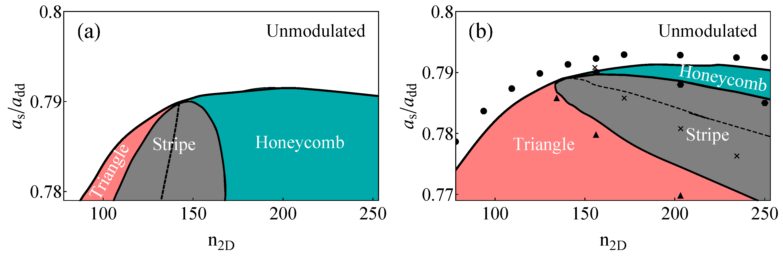
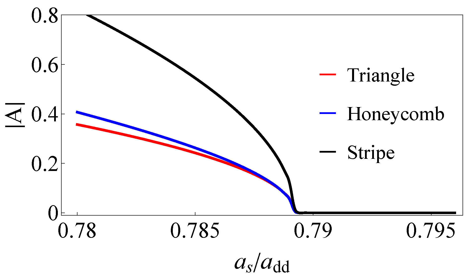
We can perform the same analysis for a square, i.e., $P(x,y)=A{\sum }_{j=1}^{2}cos({\mathbf{k}}_j·{\mathbf{r}}_{\perp }+{\theta }_j)$ with $|{\mathbf{k}}_1|=|{\mathbf{k}}_2|$ and ${\mathbf{k}}_{1,2}$ being orthogonal to each other and the stripe lattice, i.e., $P(x,y)=Acos(\mathbf{k}·{\mathbf{r}}_{\perp }+\theta )$, which leads to

$$\begin{array}{cc}\hfill \frac{\Delta E_{\mathrm{square}}}{N}=& A^2\left[\frac{k^2}{8}+\frac{3g{n}_{2\mathrm{D}}}{10{\sigma }_z}+\frac{45\pi \gamma }{256}{\left(\frac{3n_{2\mathrm{D}}}{4{\sigma }_z}\right)}^{3/2}+\frac{3g_{\mathrm{dd}}{n}_{2\mathrm{D}}}{8{\sigma }_z}\left(f\left(k{\sigma }_z\right)-\frac{4}{15}\right)\right]\hfill \\ \hfill & +A^4\left[\frac{3k^2}{32}-\frac{135\pi \gamma }{16384}{\left(\frac{3n_{2\mathrm{D}}}{4{\sigma }_z}\right)}^{3/2}\right].\hfill \end{array}$$

(13)

$$\begin{array}{cc}\hfill \frac{\Delta E_{\mathrm{stripe}}}{N}=& A^2\left[\frac{k^2}{16}+\frac{3g{n}_{2\mathrm{D}}}{20{\sigma }_z}+\frac{45\pi \gamma }{512}{\left(\frac{3n_{2\mathrm{D}}}{4{\sigma }_z}\right)}^{3/2}+\frac{3g_{\mathrm{dd}}{n}_{2\mathrm{D}}}{16{\sigma }_z}\left(f\left(k{\sigma }_z\right)-\frac{4}{15}\right)\right]\hfill \\ \hfill & +A^4\left[\frac{k^2}{64}-\frac{45\pi \gamma }{32768}{\left(\frac{3n_{2\mathrm{D}}}{4{\sigma }_z}\right)}^{3/2}\right]\hfill \end{array}$$

(14)

We note that the cubic contribution in this case vanishes. Therefore, the variational prediction in this case is that the phase transition from the unmodulated superfluid state to the modulated square or stripe state is always of the second order. Such a second-order phase transition occurs when the coefficient of $A^2$ changes its sign. Note that the kinetic energy no longer gives rise to a cubic term in the small amplitude $\mathcal{O}\left(A^3\right)$. Of course, this is a direct consequence of the specific ansatz we chose, and there is a systematic overestimation of the region of continuous transitions. One has to be cautious that its validity is only given close to the second-order point.

4. Discussion

In this section, we discuss the validity of our variational approach by comparing the results of the full-order ansatz, the small-amplitude expansion, and the numerical simulation.

In order to identify regions where the small-amplitude expansion is appropriate, we performed a variational analysis using the energy functional Equation (1), simply minimized using an expansion to the infinite order, and compared its result to the small-amplitude expansion presented in the last subsection. The full numerical results have already been published elsewhere [44,45], and we only add them in this work to benchmark our variational results.

The situation is sketched in Figure 2. The phase diagram obtained from the small amplitude approximation, i.e., the fourth-order perturbation energy from Equation (11), is displayed in Figure 2a. One can note that such a fourth-order theory predicts three modulated ground states (i.e., triangle, stripe, and honeycomb states) in addition to the trivial unmodulated state. The phase boundaries associated with these different symmetry-broken states are depicted with black lines. It is worth emphasizing that the triangle, stripe, and honeycomb states coexist at a common critical point (i.e., $n_{2\mathrm{D}}=140.5$, $a_s/a_{\mathrm{dd}}=0.789$), which is identical to the second-order point mentioned before. The characteristic behaviour associated with a second-order phase transition is the gradual continuous change of the modulation amplitude across the critical point, as shown in Figure 3. Before proceeding, we would like to point out that the triangle and honeycomb states remained stable in the stripe ground state regime with higher energy as well, and their energies crossed at the black dashed line.

To check the validity of the simple fourth-order perturbation theory, we calculated the total shift to the energy due to amplitude modulation to infinite order as well. The corresponding regime of each ground state is shown in Figure 2b. By comparing panels (a) and (b), one can readily notice the large difference between the fourth-order prediction and the calculation containing all orders in modulation amplitude. Although they yield the same second-order point, as well as the same phase boundary between the unmodulated flat state and the respective modulated states, the stripe phase moved towards a higher density region, thus giving space to a largely expanded triangular lattice. In addition to that, we also computed the border of each state numerically via imaginary time propagation, the results of which are shown by the dots in Figure 2b. The triangle, hexagon, and circle markers stand for the transition points between different ground states, while the crosses represent the critical point where the triangle and honeycomb states have the same energy as the metastable states. One can notice that, apart from a small shift in the second-order point, the full (or infinite-order) variational analysis agrees with the numerical result quite well, whereas the fourth-order perturbation ansatz can qualitatively predict the existence of various ground states. However, a quantitative comparison illustrates its deficiency.

Evidently, the reason as to why the fourth-order perturbation theory deviated substantially is due to the fact that it is valid only around the second-order point where the modulation amplitude is sufficiently small, as emphasized before. Hence, when the modulation amplitude increases as the interaction strength or density moves away from the second-order point (e.g., see Figure 3), the contributions of higher orders in amplitude A in Equations (11) and (14) can no longer be neglected. This becomes clear when comparing Figure 2a,b.

5. Conclusions

We have derived a perturbative variational ansatz (or small amplitude approximation) in detail to complement works that have already been published. This small amplitude approximation permits a qualitative understanding of the curious behaviour displayed by dipolar BECs in the thermodynamic limit: One can reveal why quantum fluctuations give rise to a second-order point, stabilise new phases such as stripes or honeycombs, and can determine which phases one can expect. However, as expected, the fourth order failed to deliver quantitatively satisfactory results, in particular when the modulation amplitude was not small compared to the background.

We established that by comparing the results of an expansion to the fourth order in amplitude (small-amplitude expansion) with a full variational analysis (to infinite order), as well as by employing rigorous numerical results. We demonstrated that the full variational perturbative result agrees with the numerical result reasonably well. Furthermore, such a perturbative approach also reveals the underlying role of quantum fluctuations in the emergence of novel states, i.e., the Lee–Huang–Yang correction can alter the energies of triangle and honeycomb states.

In summary, in this setting, the combination of a small-amplitude expansion and a full variational analysis to the infinite order proved to be a simple and extremely useful tool to analyze and understand the physics of dipolar BECs without the need to employ computationally expensive numerical simulations. Similar tools might be useful to the study of emergent phenomena in similar systems, such as multi-component dipolar BECs [57,58] or other long-range interacting quantum gases [59,60], as well as in phase–field crystal models [61].

References

1. Turing, A.M. The Chemical Basis of Morphogenesis. Philos. Trans. R. Soc. Lond. Ser. B-Biol. Sci. 1952, 23, 237. [Google Scholar] [CrossRef]
2. Pismen, L.M. Patterns and Interfaces in Dissipative Dynamics, 1st ed.; Springer: Berlin/Heidelberg, Germany, 2006. [Google Scholar] [CrossRef] [Green Version]
3. Cross, M.C.; Hohenberg, P.C. Pattern formation outside of equilibrium. Rev. Mod. Phys. 1993, 65, 851–1112. [Google Scholar] [CrossRef] [Green Version]
4. Andreev, A.F.; Lifshitz, I.M. Quantum theory of defects in crystals. Sov. Phys. JETP 1969, 29, 1107–1113. [Google Scholar] [CrossRef]
5. Leggett, A.J. Can a solid be “superfluid”? Phys. Rev. Lett. 1970, 25, 1543–1546. [Google Scholar] [CrossRef] [Green Version]
6. Chester, G.V. Speculations on Bose-Einstein condensation and quantum crystals. Phys. Rev. A 1970, 2, 256–258. [Google Scholar] [CrossRef]
7. O’Dell, D.; Giovanazzi, S.; Kurizki, G.; Akulin, V.M. Bose-Einstein Condensates with 1/r Interatomic Attraction: Electromagnetically Induced “Gravity”. Phys. Rev. Lett. 2000, 84, 5687–5690. [Google Scholar] [CrossRef] [Green Version]
8. Maucher, F.; Henkel, N.; Saffman, M.; Królikowski, W.; Skupin, S.; Pohl, T. Rydberg-Induced Solitons: Three-Dimensional Self-Trapping of Matter Waves. Phys. Rev. Lett. 2011, 106, 170401. [Google Scholar] [CrossRef]
9. Petrov, D.S. Quantum Mechanical Stabilization of a Collapsing Bose-Bose Mixture. Phys. Rev. Lett. 2015, 115, 155302. [Google Scholar] [CrossRef] [PubMed] [Green Version]
10. Macia, A.; Sánchez-Baena, J.; Boronat, J.; Mazzanti, F. Droplets of Trapped Quantum Dipolar Bosons. Phys. Rev. Lett. 2016, 117, 205301. [Google Scholar] [CrossRef] [Green Version]
11. Cabrera, C.R.; Tanzi, L.; Sanz, J.; Naylor, B.; Thomas, P.; Cheiney, P.; Tarruell, L. Quantum liquid droplets in a mixture of Bose-Einstein condensates. Science 2018, 359, 301–304. [Google Scholar] [CrossRef] [PubMed] [Green Version]
12. Ferioli, G.; Semeghini, G.; Masi, L.; Giusti, G.; Modugno, G.; Inguscio, M.; Gallemí, A.; Recati, A.; Fattori, M. Collisions of Self-Bound Quantum Droplets. Phys. Rev. Lett. 2019, 122, 090401. [Google Scholar] [CrossRef] [Green Version]
13. Santos, L.; Shlyapnikov, G.V.; Lewenstein, M. Roton-Maxon Spectrum and Stability of Trapped Dipolar Bose-Einstein Condensates. Phys. Rev. Lett. 2003, 90, 250403. [Google Scholar] [CrossRef] [Green Version]
14. Henkel, N.; Nath, R.; Pohl, T. Three-Dimensional Roton Excitations and Supersolid Formation in Rydberg-Excited Bose-Einstein Condensates. Phys. Rev. Lett. 2010, 104, 195302. [Google Scholar] [CrossRef] [PubMed] [Green Version]
15. Macrì, T.; Maucher, F.; Cinti, F.; Pohl, T. Elementary excitations of ultracold soft-core Bosons across the superfluid-supersolid phase transition. Phys. Rev. A 2013, 87, 061602. [Google Scholar] [CrossRef] [Green Version]
16. Cinti, F.; Macrì, T.; Lechner, W.; Pupillo, G.; Pohl, T. Defect-induced supersolidity with soft-core Bosons. Nat. Commun. 2014, 5, 3235. [Google Scholar] [CrossRef] [PubMed] [Green Version]
17. Mottl, R.; Brennecke, F.; Baumann, K.; Landig, R.; Donner, T.; Esslinger, T. Roton-Type Mode Softening in a Quantum Gas with Cavity-Mediated Long-Range Interactions. Science 2012, 336, 1570–1573. [Google Scholar] [CrossRef] [PubMed] [Green Version]
18. Landau, L. On the Theory of Superfluidity. Phys. Rev. 1949, 75, 884–885. [Google Scholar] [CrossRef]
19. Kadau, H.; Schmitt, M.; Wenzel, M.; Wink, C.; Maier, T.; Ferrier-Barbut, I.; Pfau, T. Observing the Rosenzweig instability of a quantum ferrofluid. Nature 2016, 530, 194–197. [Google Scholar] [CrossRef] [Green Version]
20. Schmitt, M.; Wenzel, M.; Böttcher, F.; Ferrier-Barbut, I.; Pfau, T. Self-bound droplets of a dilute magnetic quantum liquid. Nature 2016, 539, 259–262. [Google Scholar] [CrossRef] [Green Version]
21. Ferrier-Barbut, I.; Kadau, H.; Schmitt, M.; Wenzel, M.; Pfau, T. Observation of Quantum Droplets in a Strongly Dipolar Bose Gas. Phys. Rev. Lett. 2016, 116, 215301. [Google Scholar] [CrossRef] [Green Version]
22. Chomaz, L.; Baier, S.; Petter, D.; Mark, M.J.; Wächtler, F.; Santos, L.; Ferlaino, F. Quantum-Fluctuation-Driven Crossover from a Dilute Bose-Einstein Condensate to a Macrodroplet in a Dipolar Quantum Fluid. Phys. Rev. X 2016, 6, 041039. [Google Scholar] [CrossRef] [Green Version]
23. Tanzi, L.; Lucioni, E.; Famà, F.; Catani, J.; Fioretti, A.; Gabbanini, C.; Bisset, R.N.; Santos, L.; Modugno, G. Observation of a Dipolar Quantum Gas with Metastable Supersolid Properties. Phys. Rev. Lett. 2019, 122, 130405. [Google Scholar] [CrossRef] [PubMed] [Green Version]
24. Böttcher, F.; Schmidt, J.N.; Wenzel, M.; Hertkorn, J.; Guo, M.; Langen, T.; Pfau, T. Transient Supersolid Properties in an Array of Dipolar Quantum Droplets. Phys. Rev. X 2019, 9, 011051. [Google Scholar] [CrossRef] [Green Version]
25. Chomaz, L.; Petter, D.; Ilzhöfer, P.; Natale, G.; Trautmann, A.; Politi, C.; Durastante, G.; van Bijnen, R.M.W.; Patscheider, A.; Sohmen, M.; et al. Long-Lived and Transient Supersolid Behaviors in Dipolar Quantum Gases. Phys. Rev. X 2019, 9, 021012. [Google Scholar] [CrossRef] [Green Version]
26. Tanzi, L.; Roccuzzo, S.M.; Lucioni, E.; Famà, F.; Fioretti, A.; Gabbanini, C.; Modugno, G.; Recati, A.; Stringari, S. Supersolid symmetry breaking from compressional oscillations in a dipolar quantum gas. Nature 2019, 574, 382–385. [Google Scholar] [CrossRef] [PubMed] [Green Version]
27. Hertkorn, J.; Schmidt, J.N.; Böttcher, F.; Guo, M.; Schmidt, M.; Ng, K.S.H.; Graham, S.D.; Büchler, H.P.; Langen, T.; Zwierlein, M.; et al. Density Fluctuations across the Superfluid-Supersolid Phase Transition in a Dipolar Quantum Gas. Phys. Rev. X 2021, 11, 011037. [Google Scholar] [CrossRef]
28. Ilzhöfer, P.; Sohmen, M.; Durastante, G.; Politi, C.; Trautmann, A.; Natale, G.; Morpurgo, G.; Giamarchi, T.; Chomaz, L.; Mark, M.J.; et al. Phase coherence in out-of-equilibrium supersolid states of ultracold dipolar atoms. Nat. Phys. 2021. [Google Scholar] [CrossRef]
29. Guo, M.; Böttcher, F.; Hertkorn, J.; Schmidt, J.N.; Wenzel, M.; Büchler, H.P.; Langen, T.; Pfau, T. The low-energy Goldstone mode in a trapped dipolar supersolid. Nature 2019, 574, 386–389. [Google Scholar] [CrossRef] [Green Version]
30. Natale, G.; van Bijnen, R.M.W.; Patscheider, A.; Petter, D.; Mark, M.J.; Chomaz, L.; Ferlaino, F. Excitation Spectrum of a Trapped Dipolar Supersolid and Its Experimental Evidence. Phys. Rev. Lett. 2019, 123, 050402. [Google Scholar] [CrossRef] [Green Version]
31. Tanzi, L.; Maloberti, J.G.; Biagioni, G.; Fioretti, A.; Gabbanini, C.; Modugno, G. Evidence of superfluidity in a dipolar supersolid from nonclassical rotational inertia. Science 2021, 371, 1162–1165. [Google Scholar] [CrossRef]
32. Sohmen, M.; Politi, C.; Klaus, L.; Chomaz, L.; Mark, M.J.; Norcia, M.A.; Ferlaino, F. Birth, Life, and Death of a Dipolar Supersolid. Phys. Rev. Lett. 2021, 126, 233401. [Google Scholar] [CrossRef]
33. Bortolotti, D.C.E.; Ronen, S.; Bohn, J.L.; Blume, D. Scattering Length Instability in Dipolar Bose-Einstein Condensates. Phys. Rev. Lett. 2006, 97, 160402. [Google Scholar] [CrossRef] [Green Version]
34. Lahaye, T.; Metz, J.; Fröhlich, B.; Koch, T.; Meister, M.; Griesmaier, A.; Pfau, T.; Saito, H.; Kawaguchi, Y.; Ueda, M. d-Wave Collapse and Explosion of a Dipolar Bose-Einstein Condensate. Phys. Rev. Lett. 2008, 101, 080401. [Google Scholar] [CrossRef] [Green Version]
35. Wächtler, F.; Santos, L. Quantum filaments in dipolar Bose-Einstein condensates. Phys. Rev. A 2016, 93, 061603. [Google Scholar] [CrossRef] [Green Version]
36. Bisset, R.N.; Wilson, R.M.; Baillie, D.; Blakie, P.B. Ground-state phase diagram of a dipolar condensate with quantum fluctuations. Phys. Rev. A 2016, 94, 033619. [Google Scholar] [CrossRef] [Green Version]
37. Baillie, D.; Wilson, R.M.; Bisset, R.N.; Blakie, P.B. Self-bound dipolar droplet: A localized matter wave in free space. Phys. Rev. A 2016, 94, 021602. [Google Scholar] [CrossRef] [Green Version]
38. Saito, H. Path-Integral Monte Carlo Study on a Droplet of a Dipolar Bose–Einstein Condensate Stabilized by Quantum Fluctuation. J. Phys. Soc. Jpn. 2016, 85, 053001. [Google Scholar] [CrossRef]
39. Wächtler, F.; Santos, L. Ground-state properties and elementary excitations of quantum droplets in dipolar Bose-Einstein condensates. Phys. Rev. A 2016, 94, 043618. [Google Scholar] [CrossRef] [Green Version]
40. Baillie, D.; Blakie, P.B. Droplet Crystal Ground States of a Dipolar Bose Gas. Phys. Rev. Lett. 2018, 121, 195301. [Google Scholar] [CrossRef] [PubMed] [Green Version]
41. Lima, A.R.P.; Pelster, A. Quantum fluctuations in dipolar Bose gases. Phys. Rev. A 2011, 84, 041604(R). [Google Scholar] [CrossRef] [Green Version]
42. Lima, A.R.P.; Pelster, A. Beyond mean-field low-lying excitations of dipolar Bose gases. Phys. Rev. A 2012, 86, 063609. [Google Scholar] [CrossRef] [Green Version]
43. Sánchez-Baena, J.; Politi, C.; Maucher, F.; Ferlaino, F.; Pohl, T. Heating a dipolar quantum fluid into a solid. Nat. Commun. 2023, 14, 1868. [Google Scholar] [CrossRef]
44. Zhang, Y.C.; Maucher, F.; Pohl, T. Supersolidity around a Critical Point in Dipolar Bose-Einstein Condensates. Phys. Rev. Lett. 2019, 123, 015301. [Google Scholar] [CrossRef] [PubMed] [Green Version]
45. Zhang, Y.C.; Pohl, T.; Maucher, F. Phases of supersolids in confined dipolar Bose-Einstein condensates. Phys. Rev. A 2021, 104, 013310. [Google Scholar] [CrossRef]
46. Hertkorn, J.; Schmidt, J.N.; Guo, M.; Böttcher, F.; Ng, K.S.H.; Graham, S.D.; Uerlings, P.; Langen, T.; Zwierlein, M.; Pfau, T. Pattern formation in quantum ferrofluids: From supersolids to superglasses. Phys. Rev. Res. 2021, 3, 033125. [Google Scholar] [CrossRef]
47. Young-S., L.E.; Adhikari, S.K. Supersolid-like square- and honeycomb-lattice crystallization of droplets in a dipolar condensate. Phys. Rev. A 2022, 105, 033311. [Google Scholar] [CrossRef]
48. Gallemí, A.; Santos, L. Superfluid properties of a honeycomb dipolar supersolid. Phys. Rev. A 2022, 106, 063301. [Google Scholar] [CrossRef]
49. Norcia, M.A.; Politi, C.; Klaus, L.; Poli, E.; Sohmen, M.; Mark, M.J.; Bisset, R.N.; Santos, L.; Ferlaino, F. Two-dimensional supersolidity in a dipolar quantum gas. Nature 2021, 596, 357–361. [Google Scholar] [CrossRef]
50. Schmidt, J.N.; Hertkorn, J.; Guo, M.; Böttcher, F.; Schmidt, M.; Ng, K.S.H.; Graham, S.D.; Langen, T.; Zwierlein, M.; Pfau, T. Roton Excitations in an Oblate Dipolar Quantum Gas. Phys. Rev. Lett. 2021, 126, 193002. [Google Scholar] [CrossRef]
51. Biagioni, G.; Antolini, N.; Alaña, A.; Modugno, M.; Fioretti, A.; Gabbanini, C.; Tanzi, L.; Modugno, G. Dimensional Crossover in the Superfluid-Supersolid Quantum Phase Transition. Phys. Rev. X 2022, 12, 021019. [Google Scholar] [CrossRef]
52. Klaus, L.; Bland, T.; Poli, E.; Politi, C.; Lamporesi, G.; Casotti, E.; Bisset, R.N.; Mark, M.J.; Ferlaino, F. Observation of vortices and vortex stripes in a dipolar condensate. Nat. Phys. 2022, 18, 1453–1458. [Google Scholar] [CrossRef] [PubMed]
53. Lahaye, T.; Menotti, C.; Santos, L.; Lewenstein, M.; Pfau, T. The physics of dipolar Bosonic quantum gases. Rep. Prog. Phys. 2009, 72, 126401. [Google Scholar] [CrossRef]
54. Lee, T.D.; Yang, C.N. Many-Body Problem in Quantum Mechanics and Quantum Statistical Mechanics. Phys. Rev. 1957, 105, 1119–1120. [Google Scholar] [CrossRef]
55. Lee, T.D.; Huang, K.; Yang, C.N. Eigenvalues and Eigenfunctions of a Bose System of Hard Spheres and Its Low-Temperature Properties. Phys. Rev. 1957, 106, 1135–1145. [Google Scholar] [CrossRef]
56. Sachdev, S. Quantum Phase Transitions, 2nd ed.; Cambridge University Press: Cambridge, UK, 2011. [Google Scholar] [CrossRef] [Green Version]
57. Bisset, R.N.; Ardila, L.A.P.; Santos, L. Quantum Droplets of Dipolar Mixtures. Phys. Rev. Lett. 2021, 126, 025301. [Google Scholar] [CrossRef]
58. Smith, J.C.; Baillie, D.; Blakie, P.B. Quantum Droplet States of a Binary Magnetic Gas. Phys. Rev. Lett. 2021, 126, 025302. [Google Scholar] [CrossRef]
59. Han, W.; Zhang, X.F.; Wang, D.S.; Jiang, H.F.; Zhang, W.; Zhang, S.G. Chiral Supersolid in Spin-Orbit-Coupled Bose Gases with Soft-Core Long-Range Interactions. Phys. Rev. Lett. 2018, 121, 030404. [Google Scholar] [CrossRef] [Green Version]
60. Mivehvar, F.; Piazza, F.; Donner, T.; Ritsch, H. Cavity QED with quantum gases: New paradigms in many-body physics. Adv. Phys. 2021, 70, 1–153. [Google Scholar] [CrossRef]
61. Steinberg, A.B.; Maucher, F.; Gurevich, S.V.; Thiele, U. Exploring bifurcations in Bose–Einstein condensates via phase field crystal models. Chaos Interdiscip. J. Nonlinear Sci. 2022, 32, 113112. [Google Scholar] [CrossRef]
Figure 1. Sketch of the modulated density profiles 1 + P ( x , y ) with the modulation P ( x , y ) featuring either a triangular symmetry [see Equation (10)] or a stripe symmetry (c). The triangular state in (a) and the honeycomb state in (b) correspond to positive and negative modulation amplitude A, respectively. Here, the blue (white) color represents the high (low) density.
Atoms 11 00102 g001
Figure 2. Phase diagram as function of a s / a dd and n 2 D . We illustrate the error of the different methods by comparing the variational approach to the small-amplitude prediction [lines in (a)], infinite order [lines in (b)] and the full numerics [dots in (b)]. Here, the solid lines represent the boundaries between different ground states, while the dashed line indicates the location where the energy crosses between the metastable triangle and honeycomb states; the black triangles, hexagons, circles and crosses represent the numerically obtained respective phase boundaries.
Atoms 11 00102 g002
Figure 3. Dependence of the variational modulus of the amplitudes of the triangle, honeycomb, and stripe pattern on a s / a dd at fixed 2D density n 2 D = 140.5 . The phase transition is of second order.
Atoms 11 00102 g003
Disclaimer/Publisher’s Note: The statements, opinions and data contained in all publications are solely those of the individual author(s) and contributor(s) and not of MDPI and/or the editor(s). MDPI and/or the editor(s) disclaim responsibility for any injury to people or property resulting from any ideas, methods, instructions or products referred to in the content.