
Improved Line Intensity Analysis of Neutral Helium by Incorporating the Reabsorption Processes in a Helium Collisional-Radiative Model

Abstract
:1. Introduction
2. Experiment
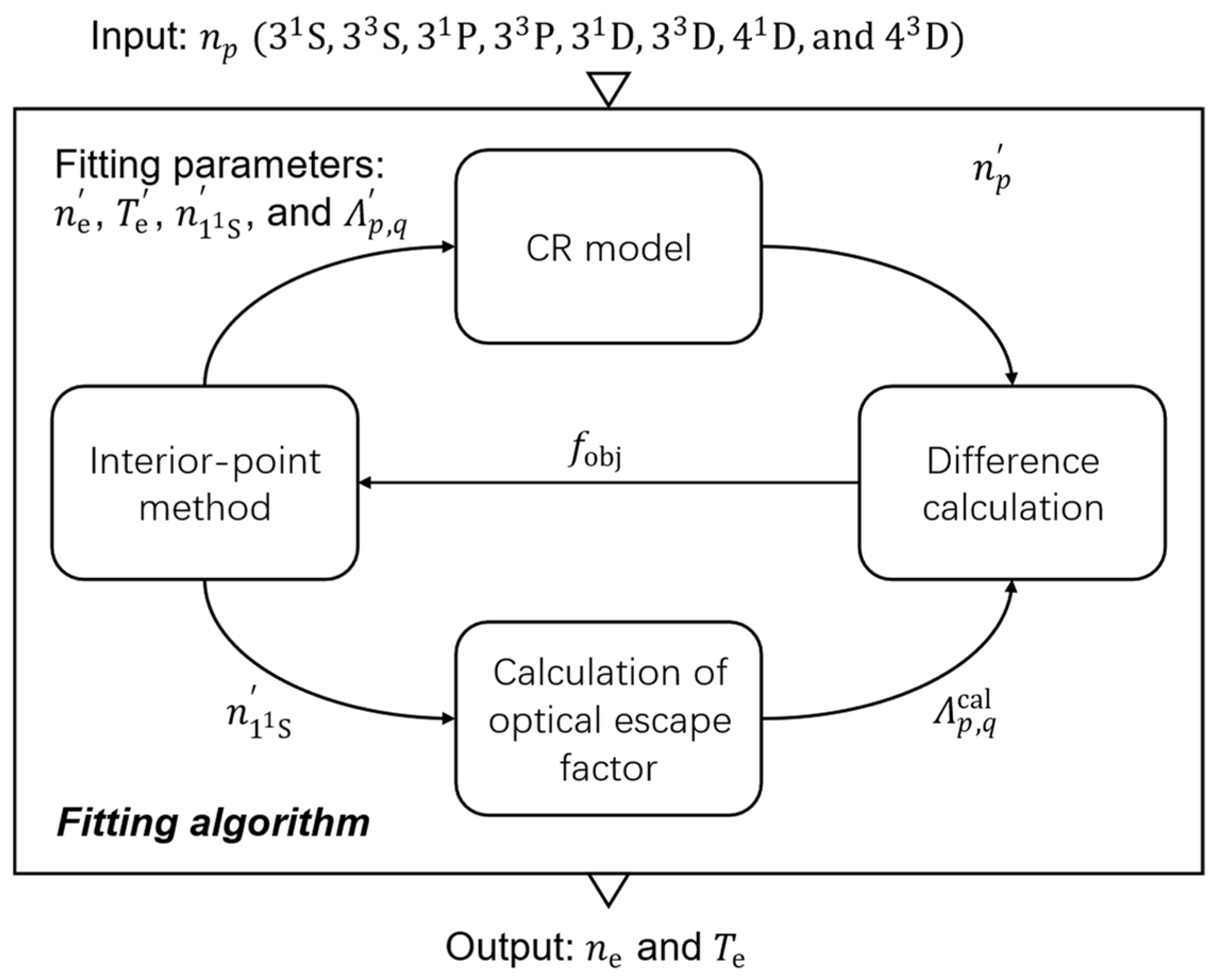
3. Model Extension
3.1. Optical Escape Factor
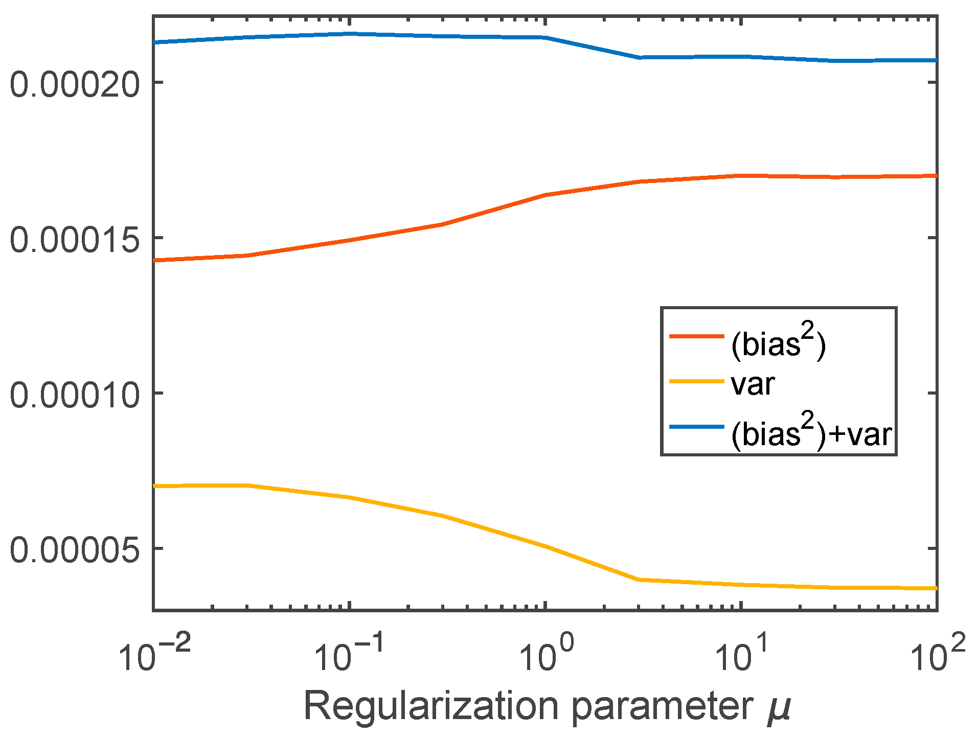
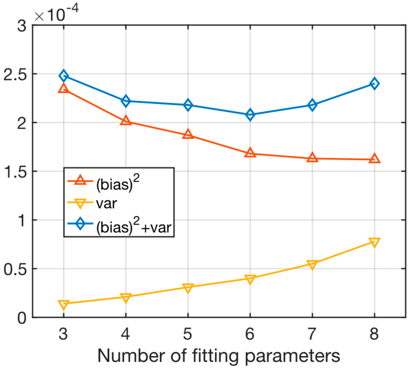
3.2. Bias–Variance Analysis
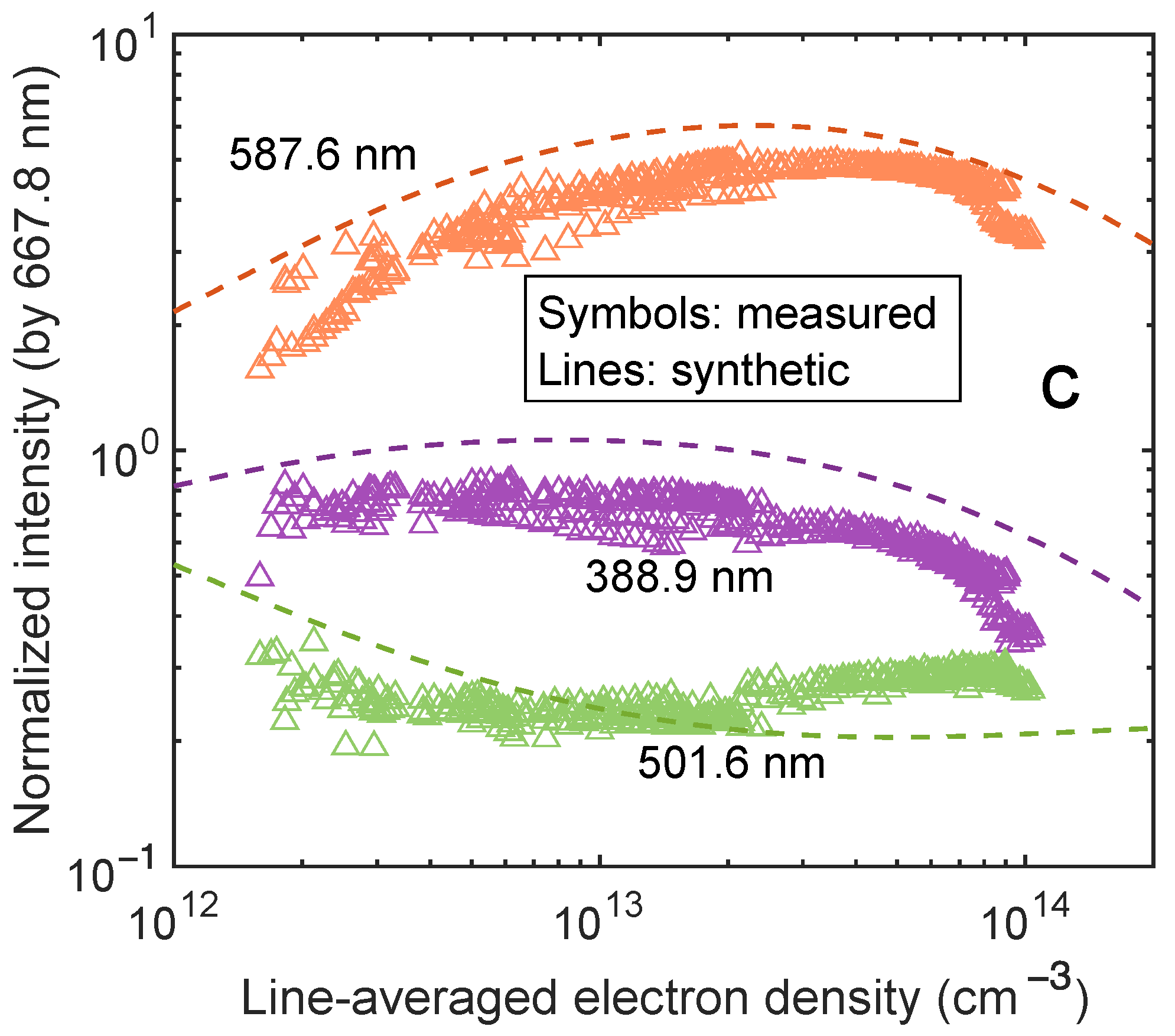
4. Results and Discussion
5. Conclusions
Author Contributions
Funding
Institutional Review Board Statement
Informed Consent Statement
Data Availability Statement
Conflicts of Interest
References
- Lin, K.; Nezu, A.; Akatsuka, H. Optical emission spectroscopy diagnosis of low-pressure microwave discharge helium plasma based on collisional-radiative model. Jpn. J. Appl. Phys. 2022, 61, 116001. [Google Scholar] [CrossRef]
- Yuji, T.; Fujii, S.; Mungkung, N.; Akatsuka, H. Optical emission characteristics of atmospheric-pressure nonequilibrium microwave discharge and high-frequency DC pulse discharge plasma jets. IEEE Trans. Plasma Sci. 2009, 37, 839–845. [Google Scholar] [CrossRef]
- Goto, M.; Morita, S. Determination of the hydrogen and helium ion densities in the initial and final stages of a plasma in the Large Helical Device by optical spectroscopy. Phys. Plasmas 2003, 10, 1402. [Google Scholar] [CrossRef] [Green Version]
- Onishi, H.; Yamazaki, F.; Hakozaki, Y.; Takemura, M.; Nezu, A.; Akatsuka, H. Measurement of electron temperature and density of atmospheric-pressure non-equilibrium argon plasma examined with optical emission spectroscopy. Jpn. J. Appl. Phys. 2021, 60, 026002. [Google Scholar] [CrossRef]
- Sawada, K.; Yamada, Y.; Miyachika, T.; Ezumi, N.; Iwamae, A.; Goto, M. Collisional-radiative model for spectroscopic diagnostic of optically thick helium plasma. Plasma Fusion Res. 2010, 5, 001. [Google Scholar] [CrossRef] [Green Version]
- Kajita, S.; Suzuki, K.; Tanaka, H.; Ohno, N. Helium line emission spectroscopy in recombining detached plasmas. Phys. Plasmas 2018, 25, 063303. [Google Scholar] [CrossRef]
- Lee, W.; Oh, C. Optical diagnostics of helium recombining plasmas with collisional radiative model. Phys. Plasmas 2018, 25, 113504. [Google Scholar] [CrossRef]
- Nishijima, D.; Hollmann, E.M. Determination of the optical escape factor in the He I line intensity ratio technique applied for weakly ionized plasmas. Plasma Phys. Control. Fusion 2007, 49, 791. [Google Scholar] [CrossRef]
- Goto, M. Collisional-radiative model for neutral helium in plasma revisited. J. Quant. Spectrosc. Radiat. Transf. 2003, 76, 331–344. [Google Scholar] [CrossRef]
- Fujimoto, T. A collisional-radiative model for helium and its application to a discharge plasma. J. Quant. Spectrosc. Radiat. Transfer 1979, 21, 439–455. [Google Scholar] [CrossRef]
- Ralchnko, Y.V.; Janev, R.K.; Kato, T.; Fursa, D.V.; Bray, I.; Heer, F.J.D. Cross Section Database for Collisional Processes of Helium Atom with Charged Particles. I. Electron Impact Processes; Rep. NIFS-DATA-59 2000; NISF: Nagoya, Japan, 2000. [Google Scholar]
- Shah, M.B.; Elliott, D.S.; McCallion, P.; Gilbody, H.B. Single and double ionisation of helium by electron impact. J. Phys. B 1988, 21, 2751–2761. [Google Scholar] [CrossRef]
- Fujimoto, T. Semi-Empirical Cross Section and Rate Coefficients for Excitation and Ionization by Electron Collision and Photoionization of Helium; Rep. IPP-AM-8 1978; Institute of Nagoya Physics, Nagoya University: Nagoya, Japan, 1978. [Google Scholar]
- Goto, M.; Fujimoto, T. Collisional-Radiative Model for Neutral Helium in Plasma: Excitation Cross Section and Singlet-Triplet Wave-Function Mixing; Rep. NIFS-DATA-43 1997; NISF: Nagoya, Japan, 1997. [Google Scholar]
- Goto, M.; Morita, S. Determination of the line emission locations in a large helical device on the basis of the Zeeman effect. Phys. Rev. E 2002, 65, 026401. [Google Scholar] [CrossRef]
- Schweer, B.; Mank, G.; Pospieszczyk, A.; Brosda, B.; Pohlmeyer, B. Electron temperature and electron density profiles measured with a thermal He-beam in the plasma boundary of TEXTOR. J. Nucl. Mater. 1992, 196–198, 174–178. [Google Scholar] [CrossRef]
- Goto, M.; Sawada, K. Determination of electron temperature and density at plasma edge in the Large Helical Device with opacity-incorporated helium collisional-radiative model. J. Quant. Spectrosc. Radiat. Transf. 2014, 137, 23–28. [Google Scholar] [CrossRef]
- Kajita, S.; Ohno, N. Practical selection of emission lines of He I to determine the photon absorption rate. Rev. Sci. Instrum. 2011, 82, 023501. [Google Scholar] [CrossRef] [PubMed]
- Iida, Y.; Kado, S.; Tanaka, S. Calculation of spatial distribution of optical escape factor and its application to He I collisional-radiative model. Phys. Plasmas 2010, 17, 123301. [Google Scholar]
- Irons, F.E. The escape factor in plasma spectroscopy-I. the escape factor defined and evaluated. J. Quant. Spectrosc. Radiat. Transf. 1979, 22, 1–20. [Google Scholar] [CrossRef]
- Fujimoto, T. Plasma Spectroscopy; Clarendon Press: Oxford, UK, 2004. [Google Scholar]
- Akatsuka, H.; Suzuki, M. Numerical study on population inversion and lasing conditions in an optically thick recombining helium plasma. Contrib. Plasma Phys. 1994, 34, 539–561. [Google Scholar] [CrossRef]
- Kim, S.; Koh, K.; Lustig, M.; Boyd, S.; Gorinevsky, D. An interior-point method for large-scale l1-regularized least squares. IEEE J. Sel. Top. Signal Process. 2007, 1, 606–617. [Google Scholar] [CrossRef]
- Zhang, Y. Solving large-scale linear programs by interior-point methods under the Matlab Environment. Optim. Methods Softw. 1998, 10, 1–31. [Google Scholar] [CrossRef]
- Rajasekhar Reddy, M.; Nithish Kumar, B.; Madhusudana Rao, N.; Karthikeyan, B. A new approach for bias–variance analysis using regularized linear regression. In Advances in Bioinformatics, Multimedia, and Electronics Circuits and Signals; Springer: Singapore, 2020. [Google Scholar]
- Wilson, R.C.; Hancock, E. Bias-variance analysis for controlling adaptive surface meshes. Comput. Vis. Image Underst. 2000, 77, 25–47. [Google Scholar] [CrossRef]
- Doroudi, S. The bias-variance tradeoff: How data science can inform educational debates. AERA Open 2020, 6, 1–18. [Google Scholar] [CrossRef]


| Wavelength λp,q (nm) | Transition (n2S+1L→n′2S′+1L′) | Ap,q (s−1) |
|---|---|---|
| 728.135 | 1.8291 × 10⁷ | |
| 706.525 | 2.7849 × 10⁷ | |
| 501.568 | 1.3368 × 10⁷ | |
| 388.864 | 0.9472 × 10⁷ | |
| 667.815 | 6.3676 × 10⁷ | |
| 587.566 | 7.0693 × 10⁷ | |
| 492.193 | 1.9855 × 10⁷ | |
| 447.150 | 2.4574 × 10⁷ |
| Number of Fitting Parameters | Fitting Parameter |
|---|---|
| 3 | , , |
| 4 | , , , |
| 5 | , , , , |
| 6 | , , , , , |
| 7 | , , , , , , |
| 8 | , , , , , , |
Disclaimer/Publisher’s Note: The statements, opinions and data contained in all publications are solely those of the individual author(s) and contributor(s) and not of MDPI and/or the editor(s). MDPI and/or the editor(s) disclaim responsibility for any injury to people or property resulting from any ideas, methods, instructions or products referred to in the content. |
© 2023 by the authors. Licensee MDPI, Basel, Switzerland. This article is an open access article distributed under the terms and conditions of the Creative Commons Attribution (CC BY) license (https://creativecommons.org/licenses/by/4.0/).
Share and Cite
Lin, K.; Goto, M.; Akatsuka, H. Improved Line Intensity Analysis of Neutral Helium by Incorporating the Reabsorption Processes in a Helium Collisional-Radiative Model. Atoms 2023, 11, 94. https://doi.org/10.3390/atoms11060094
Lin K, Goto M, Akatsuka H. Improved Line Intensity Analysis of Neutral Helium by Incorporating the Reabsorption Processes in a Helium Collisional-Radiative Model. Atoms. 2023; 11(6):94. https://doi.org/10.3390/atoms11060094
Chicago/Turabian StyleLin, Keren, Motoshi Goto, and Hiroshi Akatsuka. 2023. "Improved Line Intensity Analysis of Neutral Helium by Incorporating the Reabsorption Processes in a Helium Collisional-Radiative Model" Atoms 11, no. 6: 94. https://doi.org/10.3390/atoms11060094