Article

On Rayleigh–Taylor Dynamics

1
Department of Applied Mathematics & Statistics, Stony Brook University, Stony Brook, NY 11794, USA
2
Department of Mathematics and Statistics, University of Western Australia, Perth, WA 6009, Australia
*
Author to whom correspondence should be addressed.
Atoms 2023, 11(12), 155; https://doi.org/10.3390/atoms11120155
Submission received: 16 September 2023 / Revised: 29 November 2023 / Accepted: 1 December 2023 / Published: 8 December 2023

Abstract

:
In this work, we theoretically and numerically investigate Rayleigh–Taylor dynamics with constant acceleration. On the side of theory, we employ the group theory approach to directly link the governing equations to the momentum model, and to precisely derive the buoyancy and drag parameters for the bubble and spike in the linear, nonlinear, and mixing regimes. On the side of simulations, we analyze numerical data on Rayleigh–Taylor mixing by applying independent self-similar processes associated with the growth of the bubble amplitude and with the bubble merger. Based on the obtained results, we reveal the constituents governing Rayleigh–Taylor dynamics in the linear, nonlinear, and mixing regimes. We outline the implications of our considerations for experiments in plasmas, including inertial confinement fusion.

1. Introduction

Rayleigh–Taylor instability (RTI) plays an important role in a broad range of plasma processes in nature and technology under conditions of high and low energy densities [1,2,3,4,5,6]. Examples include the abundance of chemical elements in supernova remnants, the influence of irregularities in the Earth’s ionosphere on regional climate change, the formation of hot spots in inertial confinement fusion, and the efficiency of plasma thrusters [7,8,9,10,11,12]. While realistic plasma processes are necessarily electro- and magneto-dynamic, the control of Rayleigh–Taylor (RT) phenomena often require a better understanding of the fluid dynamic aspects [4]. In this work, we study, both analytically and numerically, RTI driven by constant acceleration in neutral plasma (fluid). We employ the group theory approach and the analysis of numerical data of Front Tracking simulations [4]. We reveal independent driving constituents that the RT flow possesses in the scale-dependent and self-similar regimes.
RT unstable interfaces and interfacial mixing play an important role in plasma processes at astrophysical and atomic scales [4]. In core-collapse abarzhi-2019, RT mixing of materials of the progenitor star enable conditions for synthesis of heavy mass chemical elements [7,13,14,15,16,17]. In the Sun, RT mixing is responsible for the accelerated ejection of matter in downdrafts propagating deeply inside of the convection zone [18]. In the inertial confinement fusion, the unstable interface between the hotter plasma, the colder plasma, and the ensued interfacial mixing influence the formation and shape of the hot spot [9,10,16,19,20,21,22,23,24]. In the Earth’s ionosphere, RT unstable plasma structures are directly relevant to the climate change on regional scales [25]. In plasma processes in technology, RT unstable interfaces are inherent in light–matter interaction, nanofabrication, and in the plasma discharges formed in and interacting with liquids [26,27,28,29].
In even vastly distinct physical conditions, RT flows exhibit similar features in their evolution [4,30,31,32]. RTI develops when fluids of different densities are accelerated against their density gradients [1,2]. Small perturbations at the fluid interface grow quickly. The flow proceeds to the nonlinear regime. The interface is transformed to a composition of small-scale shear-driven vortical structures and a large-scale coherent structure, with the heavy (light) fluid penetrating the light (heavy) fluid in bubbles (spikes) [3,4]. Eventually, the flow transitions to a state of intense interfacial mixing, where the amplitude of the mixing layer increases quadratically with time [5]. RT mixing is self-similar, anisotropic, heterogeneous, and sensitive to deterministic conditions [4,33].
RTI and RT mixing are challenging to study in experiment, in theory, and in simulation [4]. RT experiments impose tight requirements on the flow implementation, diagnostics, and control [6,34]. RT simulations need to track unstable interfaces, capture small-scale processes, and ensure large spans of spatial and temporal scales [31,35]. In RT theory, we have to solve a boundary value problem at the unstable freely evolving interface, identify asymptotic solutions, and capture symmetries of the singular and ill-posed RT dynamics [4].
Significant success has recently been achieved in theory, simulation, and experiments of RT dynamics [6]. In particular, the group theory approach has identified the asymptotic solutions and the invariant forms of RT dynamics in the scale-dependent and self-similar regimes, and has explained the experimental observation that RT mixing may keep order even at high Reynolds numbers [6,34,36]. The Front Tracking simulations and the associated merger model of the numerical data have provided experiments with accurate practical mechanisms for the evolution of RT mixing and found that numerical values of the mixing zone growth agreed with experiments [5].
In RT flow, two key constituents govern the specific (per unit mass) dynamics of a fluid parcel: the rate of momentum gain (a buoyant force) and the rate of momentum loss (an effective dissipation force) [4,5,37]. The buoyant force accelerates the fluid parcel, whereas the effective dissipation decelerates it and drags it from free fall [5,33]. We need to better understand whether these buoyancy and drag constituents can be treated as independent processes in the scale-dependent linear regime, scale-dependent nonlinear regime, and self-similar mixing regime. We have to examine whether the group theory approach and the analysis of data of the Front Tracking simulations are consistent with one another [5,33].
In this work, we investigate, both theoretically and numerically, RT dynamics with constant acceleration. In theoretical analysis, we employ the group theory approach to directly link the governing equations to the momentum model and to precisely derive the buoyancy and drag parameters for the bubble and spike in the linear, nonlinear, and mixing regimes [38]. In numerical analysis, we analyze 2D experimental and 3D simulation studies of RT mixing. We construct 2D and 3D merger trees illustrating the merger process. We find that predictions made by the merger model are in agreement with physical experiments and are better than previously reported. Based on our analytical and numerical results, we reveal that the buoyant force and the effective drag force are independent constituents governing RT dynamics in each of the regimes (linear, nonlinear, and mixing). We discuss the implications of our considerations for experiments in plasmas, including inertial confinement fusion [9,34].
Fluid instabilities and interfacial mixing are a subject of active research in contemporary plasma physics [4,5,10,12,13,21,22,24,27,28,39,40]. The novelty of our work is in the rigorous theoretical solution of RT dynamics and in the detailed analysis of the numerical data of Front Tracking numerical simulations. The group theory approach precisely derives from the governing equations the independent driving constituents of RT dynamics. The interpretation of the analyzed numerical data of Front Tracking simulations agrees with experiments. Our results provide extensive benchmarks for plasma processes to which RT instability and RT mixing are relevant.
Our paper has the following structure. After Introduction, we proceed to the mathematical problem of RT dynamics in Section 2. Section 3 presents the group theory approach. Section 4 provides analytical results for the buoyancy and drag parameters in linear and nonlinear RTI. Section 5 illustrates in detail the properties of special analytical solutions in the nonlinear regime. Section 6 investigates analytically the regime of self-similar mixing. Section 7 presents the numerical approach. Section 8 studies the merger process of two-dimensional bubbles and presents the two-dimensional merger trees. Section 9 focuses on the merger process of three-dimensional bubbles and presents three-dimensional merger tree figures. Section 10 investigates simulation growth rates. Section 11 reviews the merger model. Section 12 discusses the application of the merger model to experiments. Section 13 discusses the outcomes of our work. Section 14 presents the conclusions.

2. Mathematical Problem of RT Dynamics

We consider immiscible, inviscid fluids of differing densities separated by a well-defined interface. The heavier fluid sits above the lighter fluid and the entire system is subject to a time-dependent downwards acceleration field. The dynamics of such fluids are governed by conservation of mass, momentum, and energy:
ρ t + x i ( ρ v i ) = 0 ,
t ( ρ v j ) + x i ( ρ v i v j ) + P x j = 0 ,
E t + x i ( ( E + P ) v i ) = 0 ,
where i = 1 , 2 , 3 , ( x 1 , x 2 , x 3 ) = ( x , y , z ) are the spatial coordinates, t is time, ( ρ , v , P , E ) are the fields of density ρ , velocity v , pressure P, and energy density E = ρ ( e + 1 2 v 2 ) , and e is the specific internal energy [4,13,32].
It is necessary that momentum is conserved at the interface and that there can be no mass flow across it. Hence, the boundary conditions at the interface are
ρ θ ˙ | θ | + v · n = 0 , v · n = 0 , [ P ] = 0 ,
v · τ = arbitrary , W = arbitrary ,
where [ ] denotes the jump of functions across the interface; W = e + P / ρ is the specific enthalpy; n and τ are the normal and tangential unit vectors of the interface with n = θ / | θ | and n · τ = 0 ; θ = θ ( x , y , z , t ) is a local scalar function, with θ = 0 at the interface and θ > 0   ( θ < 0 ) in the bulk of the heavy (light) fluid, indicated hereafter by subscript h ( l ) . The initial conditions consist of initial perturbations of the flow fields and the interface. The flow is periodic in plane ( x , y ) normal to the z-direction, as is set by the initial conditions [4,32,38].
Instability is driven by acceleration. Acceleration can be due to a body force and be directed from the heavy to the light fluid. It can also be the acceleration of the (nearly planar) interface (i.e., the inertial acceleration) and be directed from the light to the heavy fluid. In our work, acceleration g is due to a body force and is directed from the heavy to the light fluid along the z-axis g = ( 0 , 0 , g ) . This acceleration modifies the pressure field: P P ρ g z . We assume that there are no mass sources and hence the velocity in the upper (lower) fluid moves to zero as z ( z ). The Atwood number A = ( ρ h ρ l ) / ( ρ h + ρ l ) parameterizes the ratio of the fluid densities [4,13,32].
The mathematical problem of RTI requires one to solve the system of nonlinear partial differential equations in four-dimensional space-time, the boundary value problems at the unstable nonlinear interface and at the outside boundaries, and also the ill-posed initial value problem with account for non-locality and singularities [4,13,41,42]. In our work, we solve this problem analytically by employing group theory approach [4,13] and numerically by analyzing data from Front Tracking simulations.

3. Group Theory Approach

3.1. Large-Scale Coherent Structures

The large-scale coherent structure is an array of bubbles and spikes periodic in the plane normal to the acceleration direction. The initial conditions determine the length and time scales of the problem. The length scale is the wavelength λ of the array, or the associated wave-vector k 1 , with λ k 1 . As a specific example, we consider the flow which has square symmetry, in which case the length scale λ and the wave-vector k are related as k = 2 π / λ .
The group theory approach [4,13] accurately describes both the linear and nonlinear dynamics of the unstable interface. In particular, for the nonlinear dynamics, there are families of asymptotic solutions with the number of relevant parameters defined by flow symmetry; the dynamics are multi-scale and characterized by the contributions of two macroscopic length scales, these being the spatial period and the amplitude of the interfacial coherent structure. Furthermore, in any regime, the dynamics are essentially interfacial, with intense motion of the fluids near the interface and effectively no motion away from the interface; see works [4,13].
Even for ideal incompressible fluids, with e ˙ = 0 and e = 0 , system Equations (1) and (2) are extremely challenging [4,13,32]. Even with this amount of complexity, the dynamics nevertheless have remarkable features of universality and order and can thus be approached using group theory [4]. Here, we implement the group theory approach and compare the principal resulting equation with the momentum model, the equations of which have the same symmetries and scaling transformations as conservation laws [4].

3.2. Analytical Methodology

RT dynamics are known to possess certain features of universality and order, and can be analyzed from first principles by applying group theory [4]. For scale-dependent dynamics, group theory can employ space groups to derive from governing equations a dynamical system and find its solutions. For scale-dependent and self-similar dynamics, group theory can be realized in a momentum model with the same symmetry transformations as governing equations [13].
For spatially periodic flows, scale-dependent RT dynamics are invariant with respect to space group G, whose generators are translations in the plane, rotations and reflections, and which also has anisotropy in the acceleration direction and inversion in the normal plane, such as the groups of square p 4 m m or hexagon p 6 m m in three-dimensional flows.
By deriving the structures of flow fields in the bulk from the governing equations, considering dynamics with potential velocity fields v h ( l ) = Φ h ( l ) , and applying irreducible representations of the relevant group, we can expand the flow fields as Fourier series and perform a spatial expansion in the vicinity of a regular point of the interface—the tip of a bubble or a spike with coordinates ( 0 , 0 , z 0 ( t ) ) and velocity ( 0 , 0 , v ( t ) ) with v ( t ) = z ˙ 0 ( t ) (the dot indicating a partial time derivative). This reduces the governing equations to a dynamical system for moments (each of which is a correlation function represented by an infinite sums of Fourier amplitudes) and surface variables. For square group p 4 m m , to the first order, N = 1 , the interface is z z 0 ( t ) = ζ ( t ) ( x 2 + y 2 ) and the dynamical system is
ρ h ζ ˙ 4 M 1 ζ M 2 2 = 0 , ρ l ζ ˙ 4 M ˜ 1 ζ + M ˜ 2 2 = 0 ,
( 1 + A ) M ˙ 1 2 + ζ M ˙ 0 M 1 2 2 ζ g = ( 1 A ) M 1 ˜ ˙ 2 ζ M ˜ 0 ˙ M ˜ 1 2 2 ζ g ,
M 0 = M ˜ 0 = v ( t ) .
Here, M ( M ˜ ) are the moments of the heavy (light) fluid, and v 0 ( 0 ) , ζ 0 ( 0 ) are the velocity and curvature of the interface at the tip of the bubble (spike). The system length-scale is k 1 , where the wavevector is k λ 1 and the wavelength is λ . The time scale is τ = 1 / k g . Group theory is further applied to solve the closure problem and find linear and nonlinear solutions for scale-dependent RT dynamics. The initial curvature and velocity are ζ ( t 0 ) and v ( t 0 ) , respectively, and t 0 τ is the initial time.

3.3. The Momentum Model

The momentum model [4,13,33,38] has the same symmetries and scaling transformations as the conservation laws, and balances, per unit mass, the rates of gain and loss of specific momentum. In doing so, it identifies invariant, scaling, and spectral properties of the dynamics.
The dynamics of a parcel of fluid are governed by the balance per unit mass of the rate of momentum gain μ and the rate of momentum loss μ ˜ as
d h d t = v , d v d t = μ ˜ μ ,
where h is the displacement along acceleration direction g , v is the corresponding velocity, μ ˜ and μ are the magnitudes of the rates of gain and loss of specific momentum in that direction [4,13]. Rates of gain μ ˜ and loss μ of specific momentum are associated with rates of gain ϵ ˜ and loss ϵ of specific energy as μ ˜ = ϵ ˜ / v and μ = ϵ / v . The rates of energy gain and dissipation are ϵ ˜ = B g v and ϵ = C v 3 / L , with B and C being the buoyancy and drag parameters and L being the length scale for energy dissipation. This leads to μ ˜ = B g and μ = C v 2 / L , and hence
d h d t = v , d v d t = B g C v 2 L ,
with h = h ( t ) > 0 and v = v ( t ) > 0 for t > t 0 > 0 . Length scale L for energy dissipation can be the horizontal scale (wavelength) L λ k 1 , the vertical scale (amplitude) L h , or a combination of these. Cases L λ k 1 and L h correspond to scale-dependent and scale-invariant dynamics, respectively.
The dynamical system in terms of moments and surface variables enables the study of the interplay of harmonics and asymptotic solutions, whereas the momentum model reveals explicit solutions and the asymptotic limits of RT dynamics.

3.4. Effect of Symmetry and Dimension

The group theory approach accommodates the analysis of two-dimensional and three-dimensional RT dynamics. In this work, we present analytical solutions for a three-dimensional RT flow. Two-dimensional analytical solutions can be obtained from three-dimensional solutions with proper transformations [13,38].

4. Analytical Quantities for Buoyancy and Drag

To derive expressions for buoyancy and drag parameters in RT dynamics, we directly link the dynamical system and the momentum model.

4.1. Scale-Dependent Linear Dynamics

In the dynamical system, we associate the curvature with the amplitude, k z 0 = 4 ζ / k , and retain only first-order harmonics in expressions for the moments. In the momentum model, we relate the vertical scale with amplitude h = z 0 , and the length-scale with wavevector, L = k 1 [38]. This transforms the governing equations to
h ˙ = v , v ˙ = B l g C l k v 2 , ζ = k 2 4 z 0 , v = M 0 = M ˜ 0 ,
where the buoyancy parameter is B l = A k z 0 = 4 A ζ / k with B l > 0 for bubbles and B l < 0 for spikes, and the drag parameter is constant, C l = A / 2 > 0 ; subscript l stands for linearity. By integrating these equations, we obtain solutions for RT dynamics of bubbles (spikes) moving up (down) and being concave down (up) with z 0 > 0 , v > 0 , ζ < 0 ( z 0 < 0 , v < 0 , ζ > 0 ):
z 0 ( t ) = C 1 e A k t + C 2 e A k t ,
v ( t ) = A k C 1 e A k t A k C 2 e A k t , ζ ( t ) = k 2 4 z 0 ( t ) ,
where C 1 and C 2 are determined by initial conditions z ( t 0 ) and v ( t 0 ) . These results hold for k z 0 1 and v B l g / C l k .
The formation of bubbles and spikes is defined by the initial conditions, with bubbles developing for ζ ( t 0 ) < 0 and spikes developing for ζ ( t 0 ) > 0 . For both bubbles and spikes, the magnitude of the curvature increases with time, and the magnitude of the velocity also increases.
In the linear regime, buoyancy grows with amplitude, and the constant drag is set by the initial conditions. The linear RT dynamics of bubbles and spikes are single-scale and defined by the horizontal scale—the wavelength of the coherent structure.

4.2. Scale-Dependent Nonlinear Dynamics

As time progresses, the bubble/spike amplitude increases, its curvature approaches a constant value, and RT dynamics become nonlinear.
In a dynamical system, we impose a constant curvature condition and retain higher-order harmonics in the moments. In the momentum model, we relate the vertical scale with the amplitude, h = z 0 , and the length-scale with the wavevector, L = k 1 . This transforms the governing equations to
z ˙ 0 = v , v ˙ = B n g C n k v 2 , ζ = k ξ , v = M 0 = M ˜ 0 .
For square symmetry, buoyancy parameter B n and drag parameter C n are, respectively,
B n ( A , ζ ) = 2 A ζ ( 9 k 2 64 ζ 2 ) 3 k 3 + 10 A k 2 ζ 128 A ζ 3 ,
C n ( A , ζ ) = k 3 ( 9 A k 2 48 k ζ + 64 A ζ 2 ) ( 9 k 2 64 ζ 2 ) ( 3 k 3 + 10 A k 2 ζ 128 A ζ 3 ) ,
in domain [ ζ cr , ζ cr ] with ζ cr = 3 8 k . Sub-script n stands for nonlinearity.
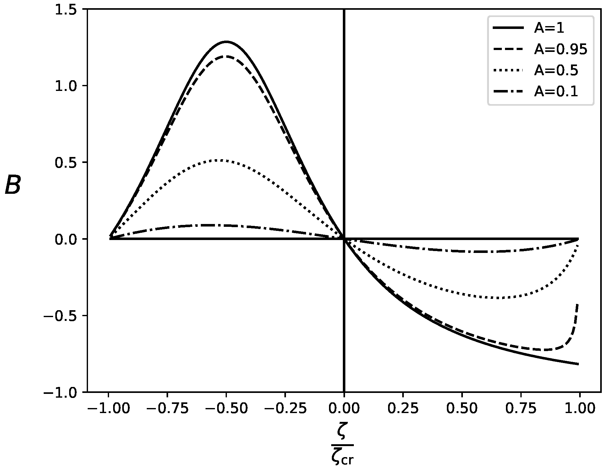
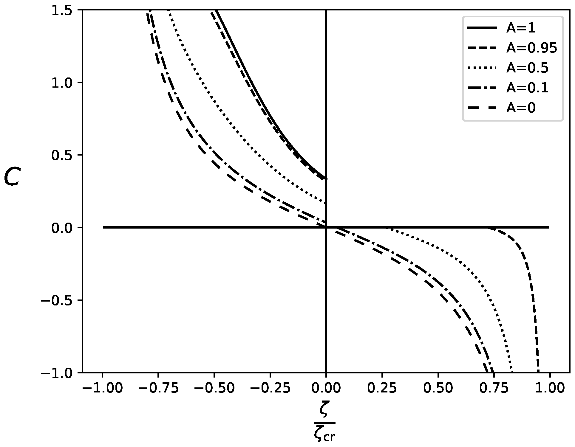
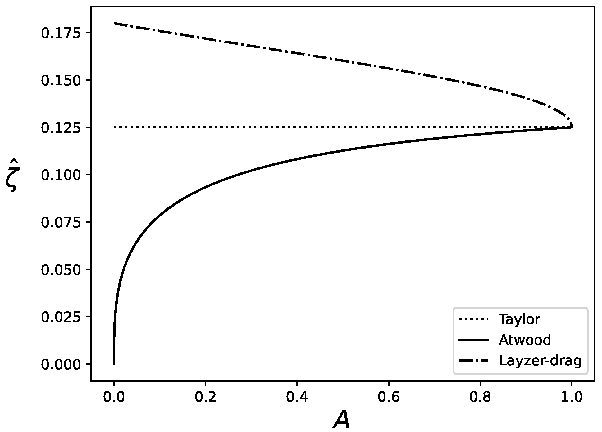
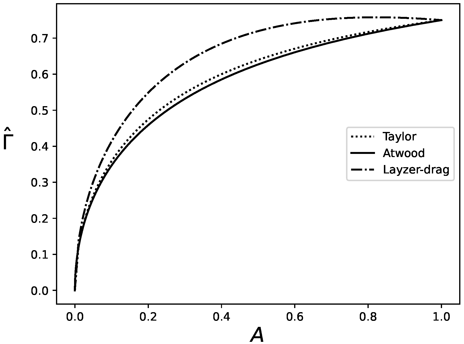
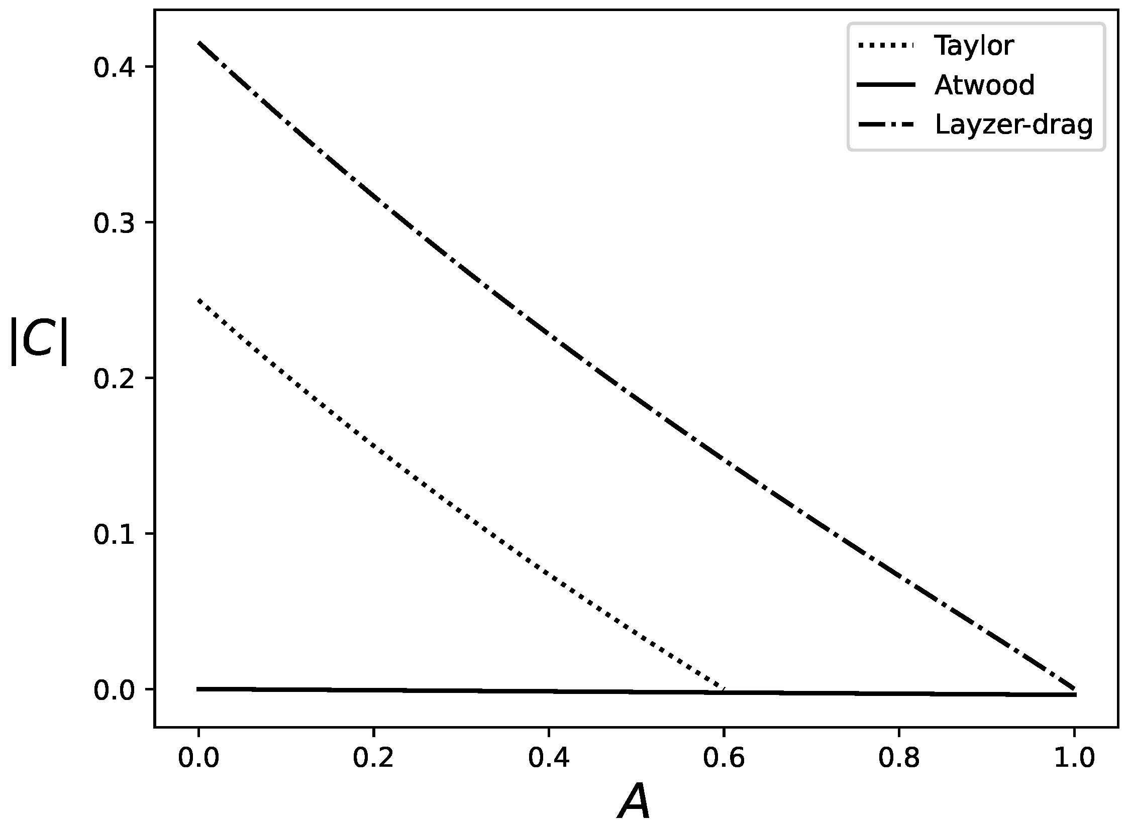
Figure 1 and Figure 2 are the plots of buoyancy and drag parameters, respectively, in nonlinear RT dynamics.
For RT bubbles, the values of buoyancy and drag parameters are B n 0 , C n 0 for ζ ( ζ cr , 0 ) with B n [ 0 , B ^ * ] , B ^ * = B ^ * ( A ) , and C n [ 0 , ) . For RT spikes, the values are B n 0 with [ B ˇ * , 0 ] , B ˇ * = B ˇ * ( A ) , for ζ ( 0 , ζ cr ) , and C n 0 with C n ( , 0 ) ] , for ζ ( ζ A , ζ cr ) . Here, ζ A = ζ A ( A ) , ζ A ( 0 , ζ cr ) is the curvature of the fastest spike; we call it the Atwood spike. A spike has unbounded velocity when the drag parameter is zero. This occurs for ζ = ζ A , where
ζ A ζ cr = 1 1 A 2 A .
Hence, we find that for nonlinear RT dynamics, there is a family of buoyancy and drag values parameterized by the interface morphology, that is, the curvature of the bubble/spike; for given ( A , ξ ) , values ( B n , C n ) are constant. The non-uniqueness is due to the presence of shear at the interface. This can be seen by defining the shear function Γ as the spatial derivative of the jump of tangential velocity at the interface. It is Γ = M ˜ 1 M 1 = 6 k 3 v / ( 9 k 2 64 ζ 2 ) near the tip of the bubble/spike.
Asymptotically, the solution of the second of Equations (9) is
v = ± B n g C n k .
For square symmetry p 4 m m , this velocity is
v = ± g k 9 k 2 64 ζ 2 k 2 2 A k ζ 64 A ζ 2 48 k ζ + 9 A k 2 ,
and the corresponding shear function is
Γ = ± 6 k g 2 A k ζ 64 A ζ 2 48 k ζ + 9 A k 2 .
In Equations (12) and (13), the positive sign applies for bubbles and the negative sign applies for spikes.
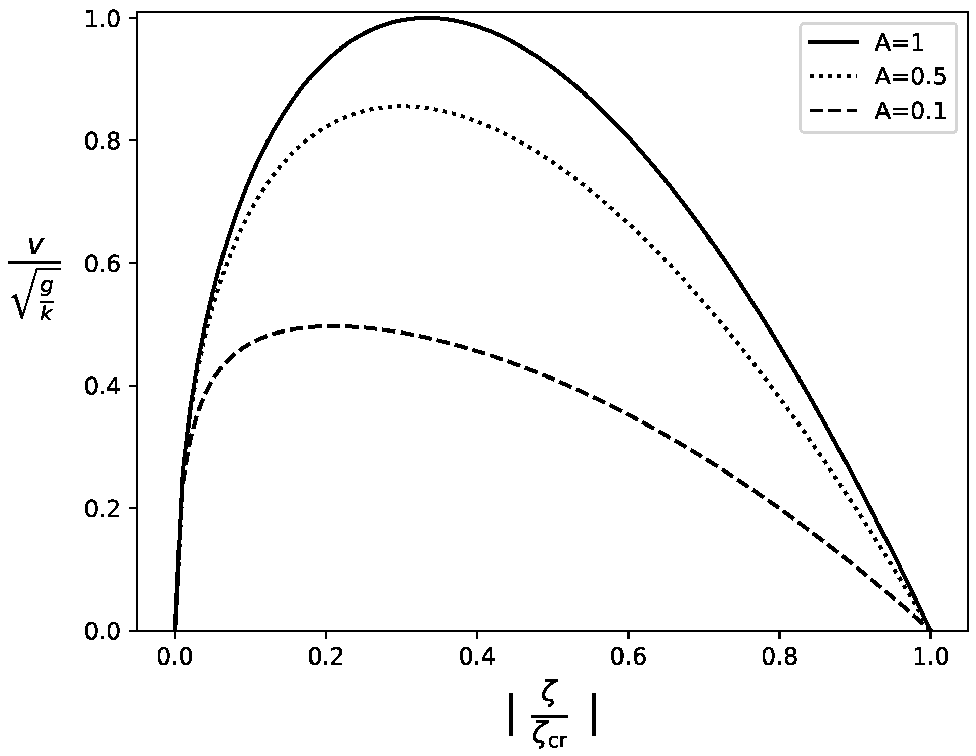
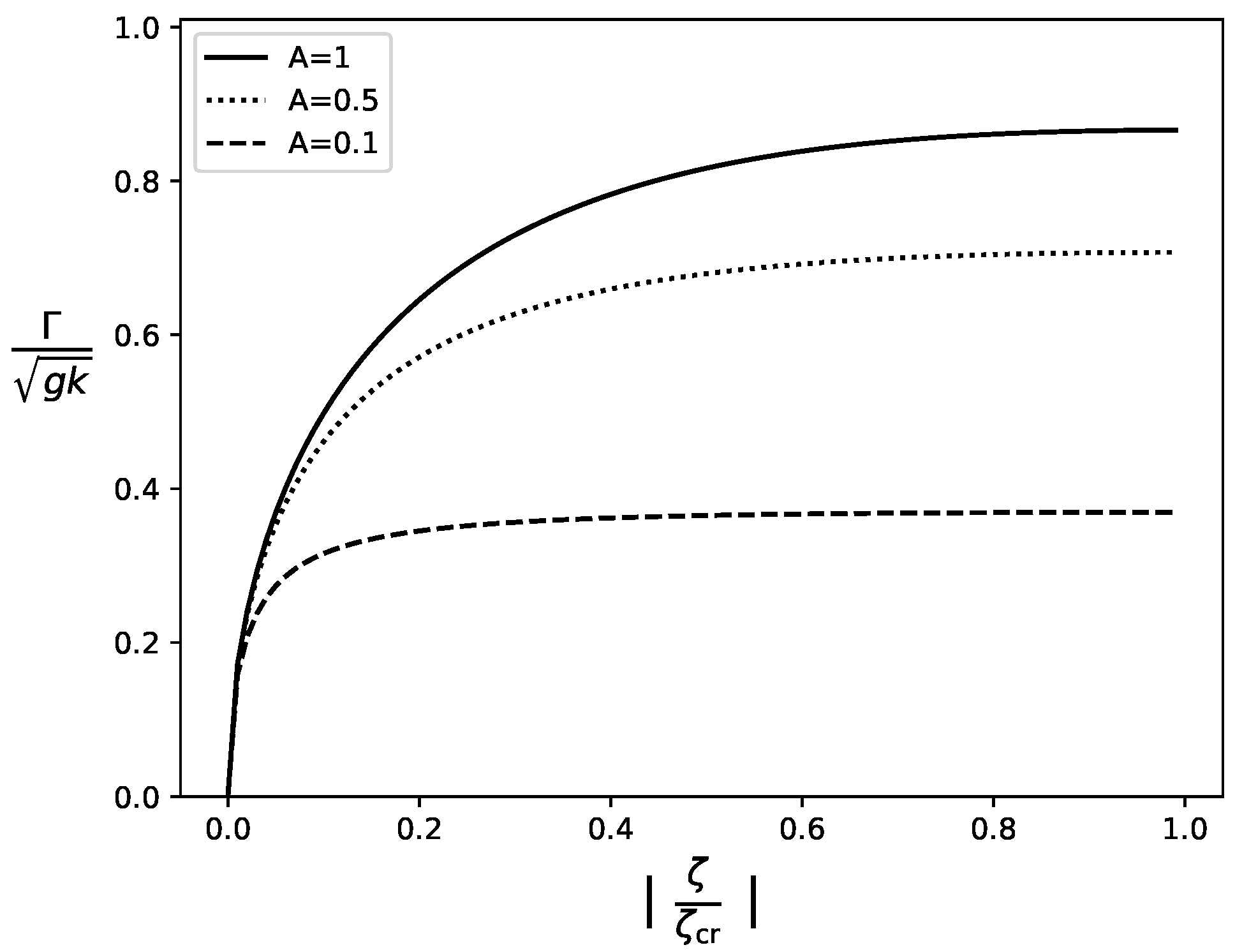
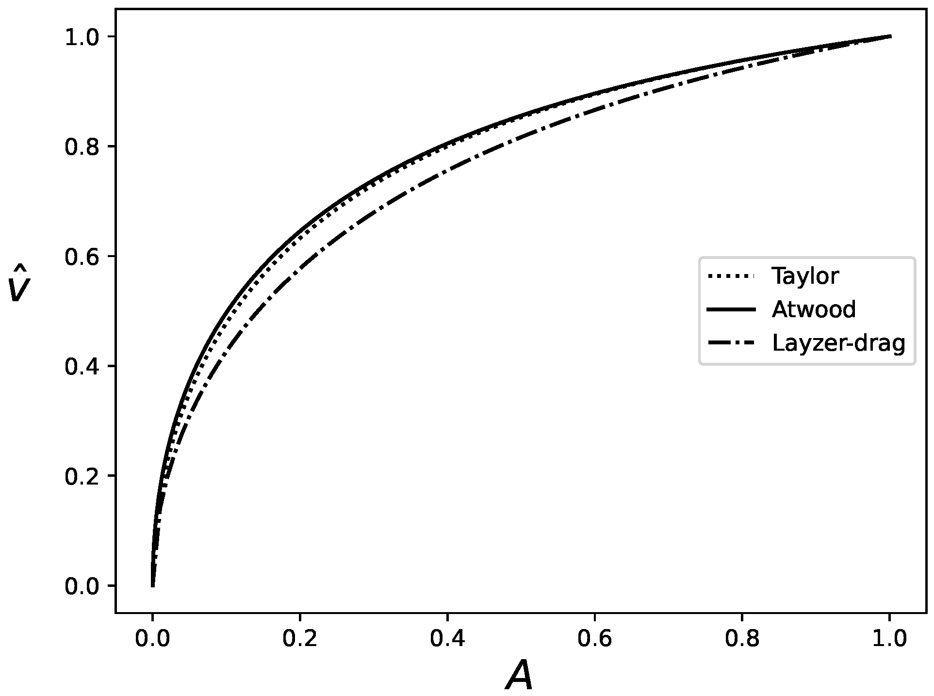
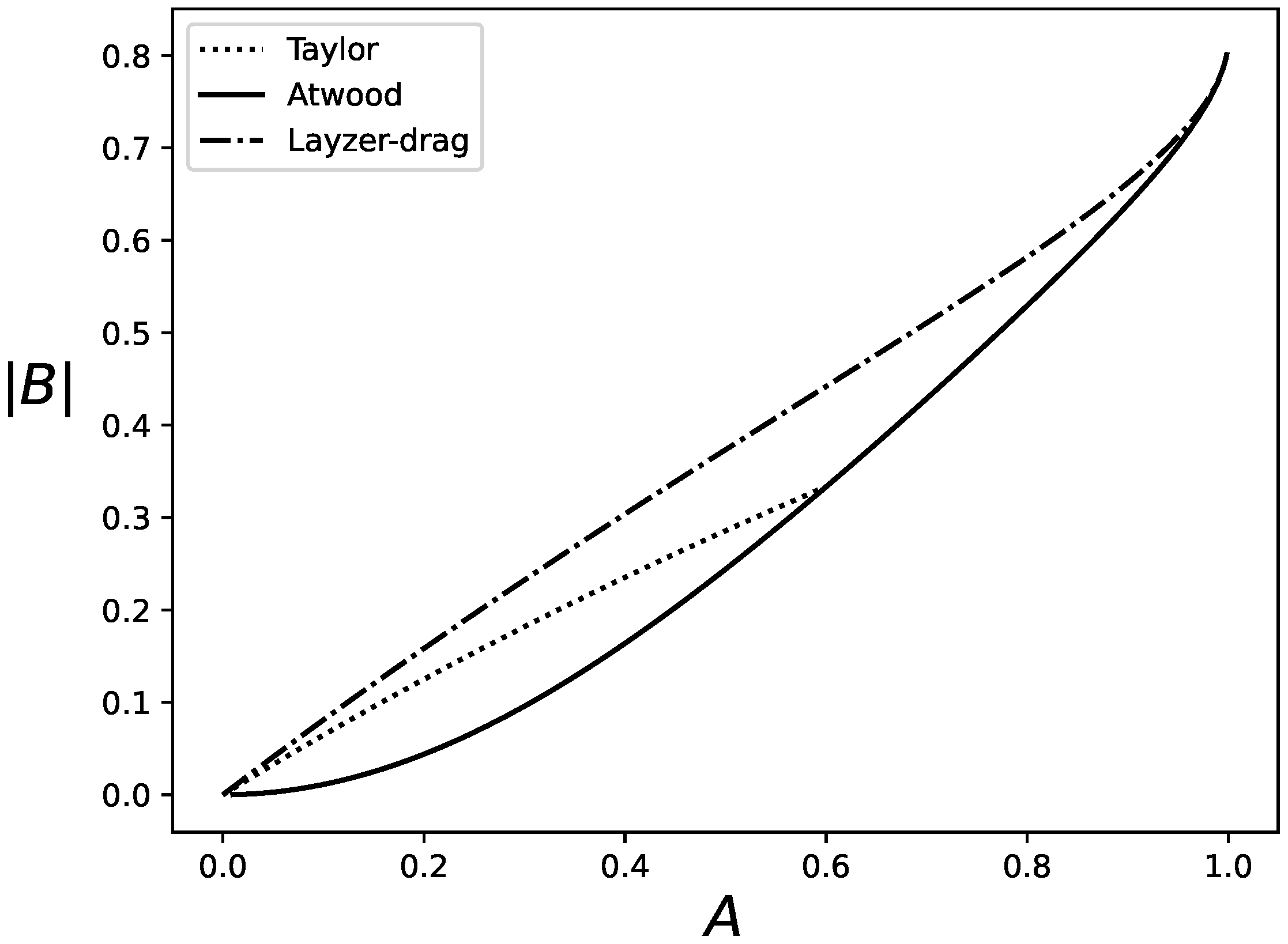
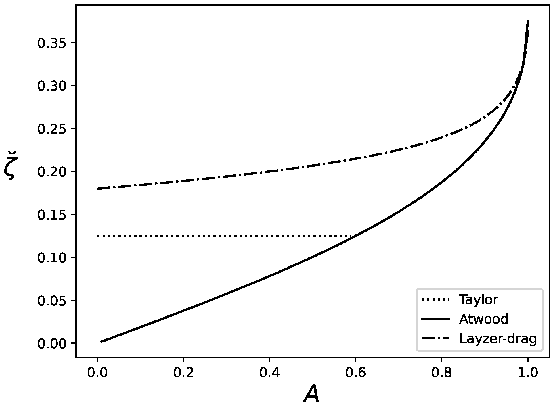
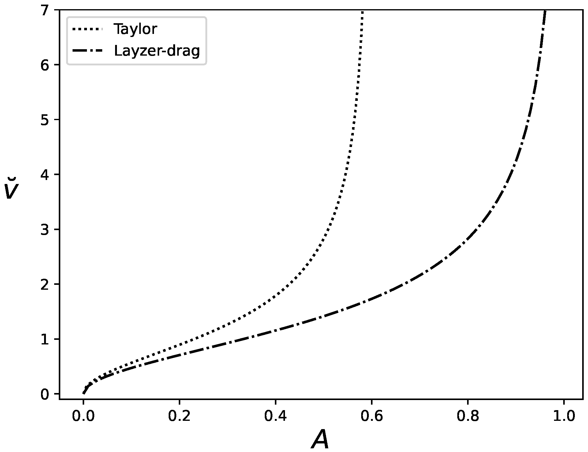
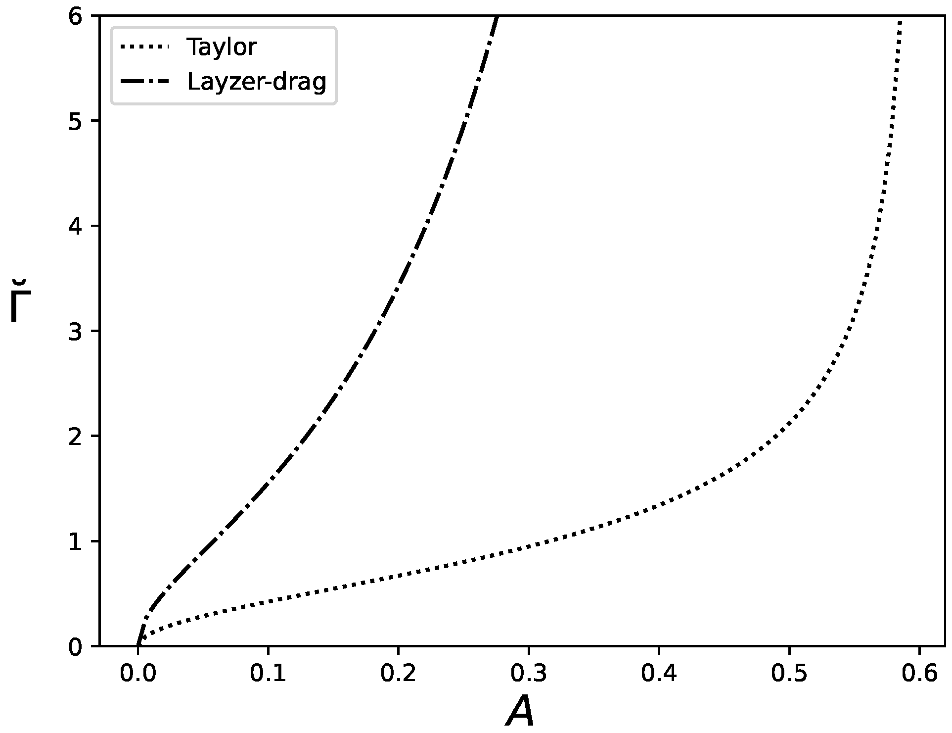
 Figure 3 and Figure 4 show the bubble tip velocity and shear function, respectively, as functions of the bubble curvature. Figure 5 and Figure 6 show the spike tip velocity and shear function, respectively, as functions of the spike curvature.
Differentiating Equation (12) with respect to ζ and setting the result to zero shows that curvature ζ vmax which maximizes velocity satisfies equation
ζ vmax 4 k A ζ vmax 3 + 9 k 2 32 ζ vmax 2 k 4 3 16 3 = 0 .
By solving this equation and substituting the solution into Equation (12), we find that the corresponding maximum velocity is
v max = 16 2 ζ vmax k 3 2 .
This is a universal relation between the curvature and the maximum velocity. We refer to this bubble as the ‘Atwood’ bubble to emphasize its dependence on the Atwood number.
RT dynamics are set by the interplay of buoyancy and drag for a given interface morphology and shear. The dynamics of RT bubbles are regular and influenced by a few competing factors: bubbles with larger curvature have larger buoyancy and move faster than flattened bubbles; yet, bubbles with larger curvature have larger shear and larger drag reducing their velocities; for curved bubbles, the shear alone can maintain the pressure at the interface, leading to zero buoyancy and infinite drag.
The dynamics of RT spikes are singular. While the magnitude of the spike’s buoyancy is qualitatively similar to that of the bubble, the spike’s drag vanishes C n 0 for ζ ζ A . This leads to a singularity indicating that the RT Atwood spike has velocity and shear growing quickly with | v | / g / k and | Γ | / k g .
The nonlinear RT dynamics of bubbles/spikes are multi-scale and defined by the two macroscopic length scales—the vertical and horizontal scales—the amplitude and wavelength of the structure, respectively. Mathematically, the (as we call it) multi-scalability is associated with the dependence of the buoyancy and the drag parameters on the interface morphology and shear. Physically, it can be understood by viewing RT coherent structures as standing waves with growing amplitudes. This reveals the mechanisms of the transition of RT dynamics from the scale-dependent to scale-invariant regimes. Particularly, the traditional merger and amplitude dominance mechanisms can both lead to the acceleration of RT bubbles/spikes due to drag force reduction, and can transfer scale-dependent dynamics L k 1 λ to scale-invariant mixing L | h | .

5. Special Solutions

We note the presence of special solutions in the nonlinear family. Some of these special solutions include the Taylor bubble/spike with curvature magnitude k / 8 , similar to works [3,38]; the Layzer-drag bubble/spike with velocity dependence 2 A / ( 1 ± A ) , similar to works [37,43]; the fastest Atwood bubble with ( ζ ^ A , v ^ A , Γ ^ A ) and the fastest Atwood spike with ( ζ ˇ A , v ˇ A , Γ ˇ A ) ; see works [13,38].

5.1. Special Solutions for Nonlinear Bubbles

We introduce nondimensional variables
ζ ^ = ζ k , v ^ = v g / k , Γ ^ = Γ k g , B ^ = B , C ^ = C .

5.1.1. The Taylor Bubble

We refer to this bubble as a ‘Taylor bubble’ since its curvature is the same as in work [3] of Davis and Taylor except for a difference in the wavevector value [4]. For the Taylor bubble, the curvature, velocity, shear function, and buoyancy and drag parameters are
ζ ^ T = 1 8 , v ^ T = 8 A 3 + 5 A , Γ ^ T = 3 4 v ^ T ,
B ^ T = 2 A 3 A , C ^ T = 3 + 5 A 4 ( 3 A ) .

5.1.2. The Layzer-Drag Bubble

The family of bubbles has a solution with velocity v ^ = 2 A / ( 1 + A ) . We call this solution the ‘Layzer-drag bubble’ since the drag model applies this velocity rescaling with the Atwood number to the single-mode Layzer first-order approximation at A = 1 [37,43]. Experiments and simulations tend to compare well with this rescaling [37,43,44]. For the Layzer-drag bubble, the curvature, velocity, and shear function are
ζ ^ L = ζ ^ L ( A ) , v ^ L = 2 A 1 + A , Γ ^ L = 6 v ^ L 9 64 ζ ^ L 2 ,
and the buoyancy and drag parameters are as defined in Equation (10). The dependence of the Layzer-drag bubble curvature on the Atwood number is cumbersome. For fluids with very different densities, A 1 , in the solution for the Layzer-drag bubble,
ζ ^ L 1 8 1 + 1 A 6 ,
v ^ L 1 1 A 4 , Γ ^ L 3 4 + 6 ( 1 A ) 32 ,
B ^ L 1 + 1 A 6 , C ^ L 1 + 1 A 6 .
For fluids with very similar densities, A 0 , in the solution for the Layzer-drag bubble,
ζ ^ L 9 4 3 8 , v ^ L 2 A , Γ ^ L 3 A 2 ,
B ^ L 8 3 ζ ^ L 3 A , C ^ L 4 3 3 ζ ^ L .
The Layzer-drag bubble is more curved for fluids with similar densities, A 0 , when compared to fluids with very different densities, A 1 . For fluids with very different densities, A 1 , the values of the curvature, velocity, shear, and group-momentum coefficients of the Layzer-drag bubble are the same as the values of the corresponding quantities of the Taylor bubble. For 0 < A < 1 , the Layzer-drag bubble is more curved and has smaller velocity and larger shear when compared to the Taylor bubble.

5.1.3. The Atwood Bubble

We refer to the fastest member of the family of solutions as the ‘Atwood bubble’ to emphasize its dependence on the Atwood number [38]. The curvature, velocity, shear function, and buoyancy and drag parameters of the Atwood bubble are
ζ ^ A = ζ ^ vmax , v ^ A = 16 2 ζ ^ A 3 , Γ ^ A = 6 v ^ A 9 64 ζ ^ A 2 ,
B ^ A = 8192 ζ ^ A 4 9 320 ζ ^ A 2 8192 ζ ^ A 4 , C ^ A = 16 ζ ^ A 9 320 ζ ^ A 2 8192 ζ ^ A 4 ,
where ζ vmax = k ζ ^ vmax is given by Equation (14). We note that
B ^ A = C ^ A v ^ A 2 .
For fluids with very different densities, A 1 , in the solution for the Atwood bubble,
ζ ^ A 1 8 1 1 A 8
v ^ A 1 3 16 ( 1 A ) , Γ ^ A 3 4 21 128 ( 1 A ) ,
B ^ A 1 13 8 ( 1 A ) , C ^ A 1 5 4 ( 1 A ) .
For fluids with very similar densities, A 0 , in the solution for the Atwood bubble,
ζ ^ A 3 16 A 1 3 , v ^ A 27 A 8 , Γ ^ A 3 A 2 ,
B ^ A 9 8 A 4 3 , C ^ A 1 3 A 1 3 .
For fluids with very different densities, A 1 , the values of the curvature, velocity, shear function, and group-momentum coefficients of the Atwood bubble are very close to the values of the corresponding quantities of the Taylor and the Layzer-drag bubbles. For fluids with a finite density ratio, the curvatures relate as ζ ^ A / ζ ^ cr ( 0 , 1 / 8 ) , ζ ^ L / ζ ^ cr ( 0 , 1 ) and ζ ^ A / ζ ^ T ( 0 , 1 ) . For 0 < A < 1 , the Atwood bubble is less curved and has larger velocity and smaller shear when compared to the Layzer-drag and the Taylor bubble.
Figure 7, Figure 8, Figure 9, Figure 10 and Figure 11 are plots of the nondimensional variables as functions of the Atwood number A for these special bubbles.

5.2. Special Solutions for Nonlinear Spikes

We introduce nondimensional variables
ζ ˇ = ζ k , v ˇ = v g / k , Γ ˇ = Γ k g , B ˇ = B , C ˇ = C .

5.2.1. The Taylor Spike

We refer to this spike as a ‘Taylor spike’ since its curvature magnitude is the same as in work [3] of Davis and Taylor except for a difference in the wavevector value [4]. For the Taylor bubble, the curvature, velocity, shear function, and buoyancy and drag parameters are
ζ ˇ T = 1 8 , v ˇ T = 8 A 3 5 A , Γ ˇ T = 3 4 v ˇ T ,
B ˇ T = 2 A 3 + A , C ˇ T = 3 5 A 4 ( 3 + A ) .
For the Taylor spike, the velocity and the shear function have non-positive values, which are zero for A 0 + , finite for 0 < A < 3 / 5 , and which become singular approaching negative infinity for A 3 / 5 .

5.2.2. The Layzer-Drag Spike

The family of spikes has amongst them a solution with velocity v = 2 A / ( 1 A ) . We call this solution the ‘Layzer-drag spike’ since the drag model applies this velocity rescaling with the Atwood number to the single-mode Layzer first-order approximation at A = 1 [37,43]. Experiments and simulations tend to compare well with this rescaling [37,43,44]. For the Layzer-drag bubble, the curvature, velocity, and shear function are
ζ ˇ L = ζ ˇ L ( A ) , v ˇ L = 2 A 1 A , Γ ˇ L = 6 v ˇ L 9 64 ζ ˇ L 2 ,
and the buoyancy and drag parameters are as defined in Equation (10). The dependence of the Layzer-drag spike curvature on the Atwood number is cumbersome. For fluids with very different densities, A 1 , in the solution for the Layzer-drag spike,
ζ ˇ L 3 8 1 2 ( 1 A ) ,
v ˇ L 2 1 A , Γ ˇ L 1 6 2 1 A ,
B ˇ L 9 11 1 4 11 2 ( 1 A ) , C ˇ L 9 22 ( 1 A ) .
For fluids with very similar densities, A 0 , in the solution for the Layzer-drag spike,
ζ ˇ L 9 4 3 8 , v ˇ L 2 A , Γ ˇ L 3 A 2 ,
B ˇ L 8 3 ζ ˇ L 3 A , C ˇ L 4 3 ζ ˇ L 3 .
The Layzer-drag spike is more curved for fluids with very different densities A 1 than for fluids with very similar densities A 0 . For a two-fluid system with A ( 0 , 1 ) , ζ ˇ L / ζ ˇ T ( 9 4 3 , 3 ) , and the Layzer-drag spike is more curved than the Taylor spike. The Layzer-drag spike has smaller absolute velocity and smaller absolute shear than the Taylor spike.
For fluids with very similar densities A 0 , the magnitude of the curvature of the Layzer-drag spike is the same as that for the Layzer-drag bubble, with ζ ˇ L = ζ ^ L . The magnitudes of the velocity and shear of the Layzer-drag spike differ from those of the Layzer-drag bubble: the velocity and shear magnitudes of the spike approach infinity for A 1 , whereas the velocity and the shear magnitudes of the bubble are finite for any A.

5.2.3. The Atwood Spike

The fastest spike is where the drag parameter is zero. Its curvature is that given in Equation (11). We refer to this spike as the ‘Atwood spike’ to emphasize its dependence on the Atwood number [13,38]. It is the fastest growing, and hence the physically significant spike. For the Atwood spike, the curvature is regular, ζ ˇ ζ ˇ A , whereas the velocity and the shear function are singular, with v ˇ A / g / k , for any Atwood number.
For fluids with very different densities, A 1 , the solution for the Atwood spike is
ζ ˇ A = 3 8 1 2 ( 1 A ) , B A = 9 11 1 4 11 2 ( 1 A ) .
For fluids with very similar densities, A 0 , the solution for the Atwood spike is
ζ ˇ A = 3 16 A , B A = 9 8 A 2 .
The Atwood spike is less curved than the Layzer-drag spike for A [ 0 , 1 ) and has the same curvature as the Layzer-drag spike ζ ˇ A / ζ ˇ L = 1 at A = 1 . The Atwood spike attains the same curvature as the Taylor spike ζ ˇ A / ζ ˇ T = 1 at A = 3 / 5 .
The properties of the curvature, velocity, and shear of the Atwood spike differ dramatically from those of the Atwood bubble: for any density ratio A, the magnitudes of the velocity and shear of the Atwood spike are singular, whereas the magnitudes of the velocity and shear of the Atwood bubble are regular and finite. While the magnitudes of the curvature of the Atwood spike and the Atwood bubble are both finite, the Atwood spike is more curved (less curved) when compared to the Atwood bubble for fluids with very different (very similar) densities A 1 ( A 0 ) .
Figure 12, Figure 13, Figure 14, Figure 15 and Figure 16 are plots of nondimensional variables as functions of the Atwood number A for these special spikes.

6. Self-Similar Mixing

In the mixing regime, the dynamical system is generalized as
v ˙ = B m g C m v 2 h , h ˙ = v .
In the momentum model, we relate the length-scale for energy dissipation with the amplitude as L = | h | = | z 0 | , and we set B = B m , C = C m , where subscript m stands for mixing. The buoyancy and drag are free values due to the many scales contributing, with B m , C m > 0 ( < 0 ) for bubbles (spikes) with h > 0 , v > 0 ( h < 0 , v < 0 ) . Herein, we consider B m > 0 , C m > 0 , h > 0 , v > 0 . Our consideration can also be applied for B m < 0 , C m < 0 , h < 0 , v < 0 ; see works [4,33,36].
We solve the model equation in domain h , v > 0 , t > t ˜ 0 for constant B m , C m > 0 and with initial conditions h ˜ 0 = h ( t ˜ 0 ) , v ˜ 0 = v ( t ˜ 0 ) :
h ¨ + C m h ˙ 2 h B m g = 0 .
The solution is sought in the physical domain with h , v , t > 0 and with initial conditions t = t 0 , h 0 = h ( t 0 ) , and v 0 = h ˙ ( t 0 ) [4,36].
The associated homogeneous equation is h ¨ = C h ˙ 2 / h . It can be solved by the method of separation of variables leading to the general solution, with integration constants H 0 , V 0 , as
h d C + 1 H 0 C + 1 H 0 C = ( C + 1 ) V 0 ( t t 0 ) ,
where subscript d stands for dissipative dynamics. For t / t 0 1 , the solution is
h d = B d t 1 1 + C , B d = H 0 ( C + 1 ) V 0 H 0 1 C + 1 .
To find a particular solution for the non-homogeneous equation h ¨ + C h ˙ 2 / h = g , we invoke Lie group analysis and employ one-parameter scaling transformation t ^ = e ψ t , h ^ = e γ ψ h , where ψ and γ are the transformation’s parameter and constant. This leads to e ( γ 2 ) ψ ( h ¨ + C h ˙ 2 / h ) = g and hence γ = 2 and the corresponding invariant h / t 2 . The particular solution is h a = B a g t 2 / ( 2 + 4 C ) , where subscript a stands for accelerative dynamics. The general solution is a function of the dissipative and accelerative solutions, h = h ( h d , h a ) .
Whilst solutions h d and h a should be coupled because of the nonlinear nature of the differential equation, it has, in fact, the remarkable property that in the respective asymptotic regimes, ( t t 0 ) / t ) 1 and t / t 0 1 , solutions h a and h d are effectively decoupled. This decoupling is due to the distinct symmetries of the solutions, h a and h d [4,36].
For L λ , the gains and losses are fully balanced, μ = μ ˜ and ϵ = ϵ ˜ . For L h , the gains and losses are unbalanced, μ μ ˜ and ϵ ϵ ˜ [4,36]. According to data, the imbalance is small, ( μ ˜ μ ) / μ ˜ 1 [5]. This slight imbalance results in the flow acceleration and in the development of self-similar RT mixing: parcel of the heavy fluid moves in the acceleration direction, parcel of the light fluid moves against the acceleration direction, the position of the center of mass of the fluid system changes, energy is gained, almost all of this gain effectively dissipates, and its remnant leads to flow acceleration [4,36]. The transition from nonlinear RTI to RT mixing may occur via the growth of the horizontal scale, as the merger model predicts [5].

7. Numerical Approach

Assuming that acceleration is uniform in time, we recall that the penetration of the bubble interface into the heavier fluid occurs on an acceleration-determined time scale and follows a t 2 scaling law. The penetration distance of the light fluid into the heavy fluid is known to be given by
h b = α b A g t 2 ,
where A = ( ρ 2 ρ 1 ) / ( ρ 2 + ρ 1 ) is the Atwood number, a relative density difference that modifies the uniform acceleration, g. Here, ρ 1 ( ρ 2 ) denotes the density of the light (heavy) fluid. The constant α b is a growth rate parameter.
This remainder of this paper analyzes RT mixing data in depth, with archived data that could be used in future studies of bubble merger. Here, we analyze 2D experimental and 3D simulation studies of RT mixing; 2D and 3D merger trees are constructed as a result of this process. In these figures, the bubble merger process occurring over multiple time steps can be observed. Detailed analysis of all measured properties of each bubble are recorded in a spreadsheet (not included here due to its size), and will aid in any further analyses; see Section 8 and Section 9.
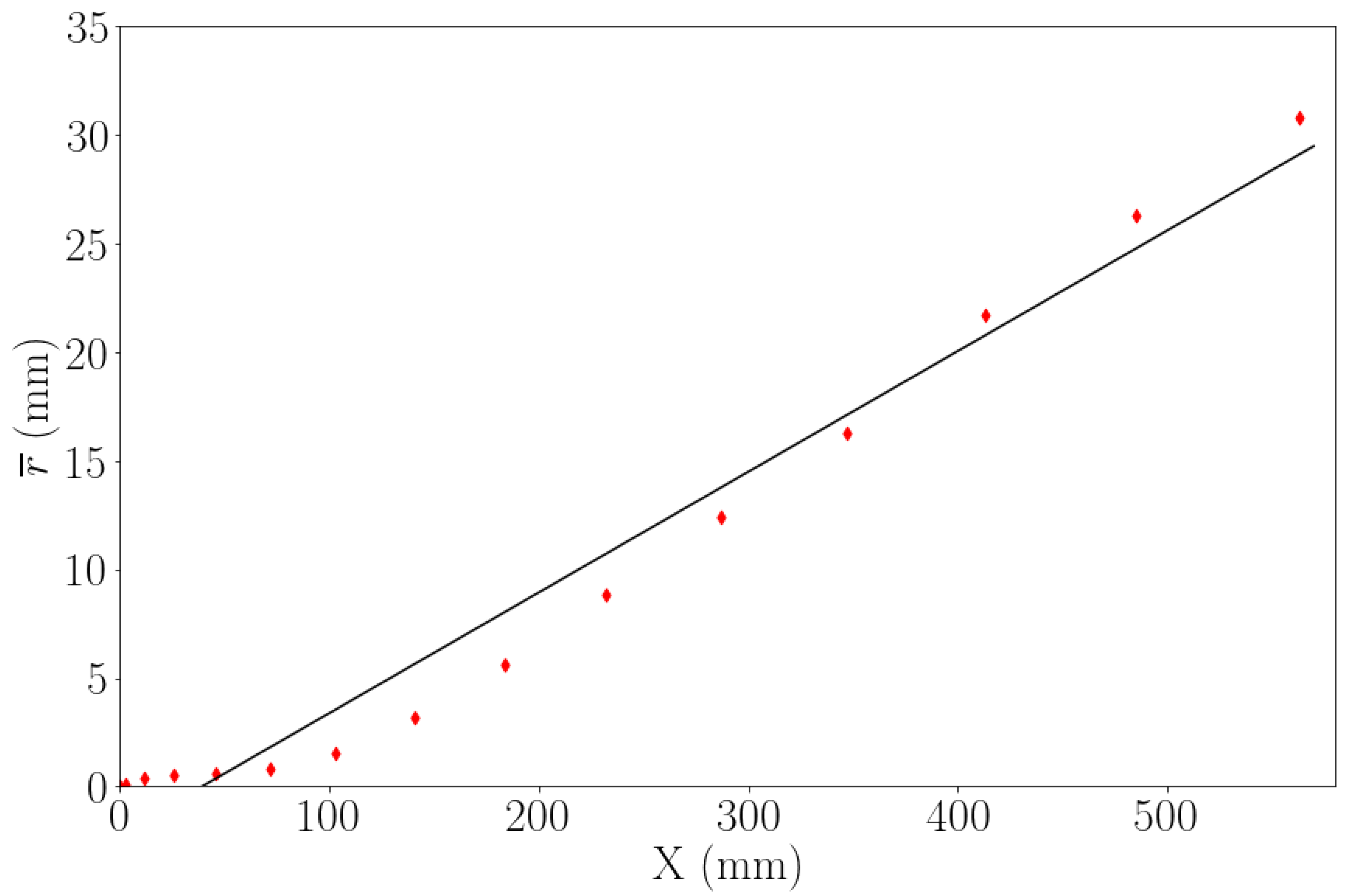
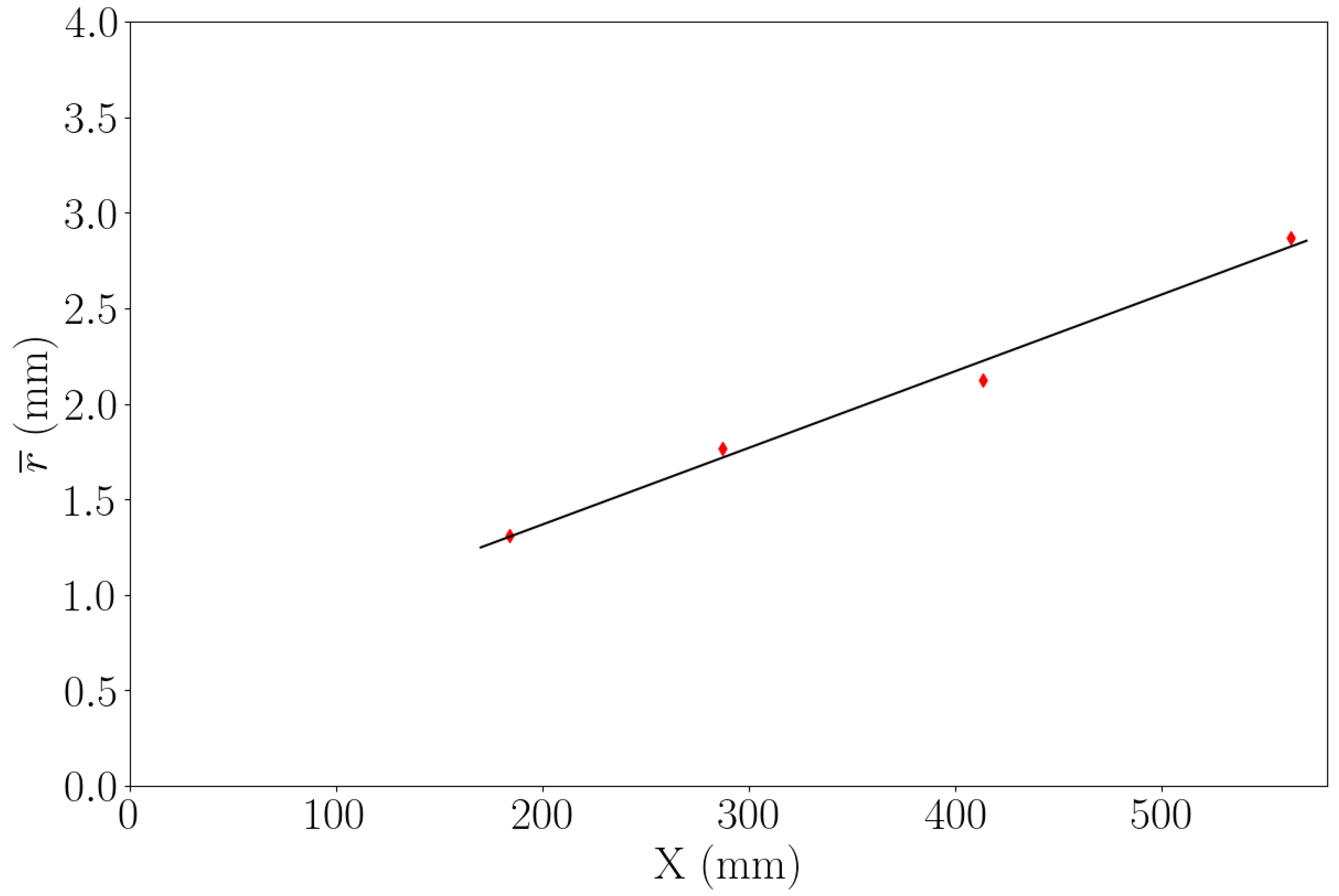
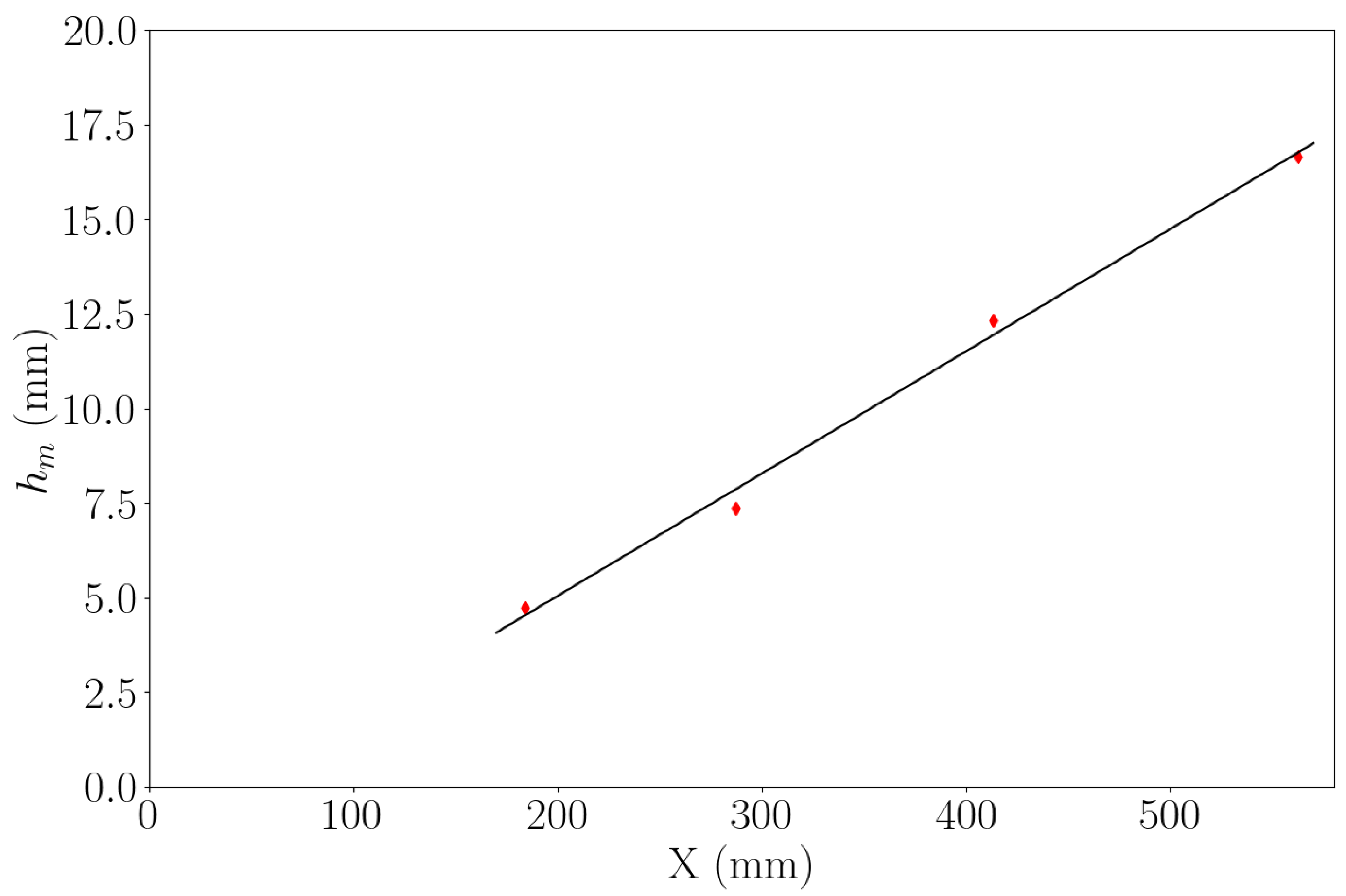
The mean bubble radius, r ¯ , and the separation height between adjacent bubbles undergoing a merger, h m , grow on a quadratic time scale [45], in common with α b . These growth rates are related by the model, with α r and α h m being their respective growth rate parameters. We determine these three growth rates for the numerically simulated experiment. The extraction and analysis of these data, including relevant plots, are presented in Section 10.
The bubble merger model correctly predicts the measured merger rates relative to experimental data. The model has one adjustable parameter, which is a noise level (fluctuation or variance) in the bubble radii. A brief overview of the merger model and all relevant equations is given in Section 11.
On a quantitative level, we revisit predictions made by the merger model and reported in [45]. We find that for the Smeeton and Youngs (SY) experiments [46], the merger model better predicts growth rate α b than originally reported. Applications of this model to numerical simulation data are also presented; see Section 12. We comment that α b is sensitive to the amplitude of long wavelength random (noise) perturbations to the initial data, as was observed in the experiments of Meusche, Andrews and Schilling [47,48,49] and the LEM experiments of Dimonte [50] whose long-wavelength noise in the experiment apparatus made its use for comparison to simulations difficult. The bubble merger model studied here excludes such initial perturbations, which appear to be missing in the SY experimental data [46] and are missing in the simulation data studied here.
We recall that the fluids are accelerated; this is customarily achieved by a rapid downward acceleration of a gravitationally stable two-fluid system, with the light fluid above the heavy. These turbulent events accelerating the bubble penetration occur at the base of the bubble, or even above the base, in the form of a vortex ring wrapping around the stem above the downward moving bubble. According to this picture, we see the origin of the randomness as lying in the fluids at the base of the bubble, or even above it, and coming from turbulent aspects of the mixing flow, a well-known source of randomness. In fact, in our data, we observe that the merger occurs in stages, starting at the base and progressing downwards to the tip. Not explored here, but likely, is the fact that the merger begins earlier, at the level of vortex rings driving the bubble.
We mention an alternate bubble merger model [37] which predicts one observed parameter ( α b ) on the basis of one input parameter: a noise level in the initial data that is assumed to originate in the initial perturbations of the initial interface. This model mispredicts the bubble radius and velocity for non-interacting bubbles. The misprediction is significant as its velocity contains a term proportional to its radius. The bubble merger model proposed by Cheng et al. [45] yields a range of predictions for the bubble height-to-width ratio that is consistent with the values observed in experiment and simulation. However, as noted in [51], the model [52,53] predicts a value for this ratio that falls outside the observed range.
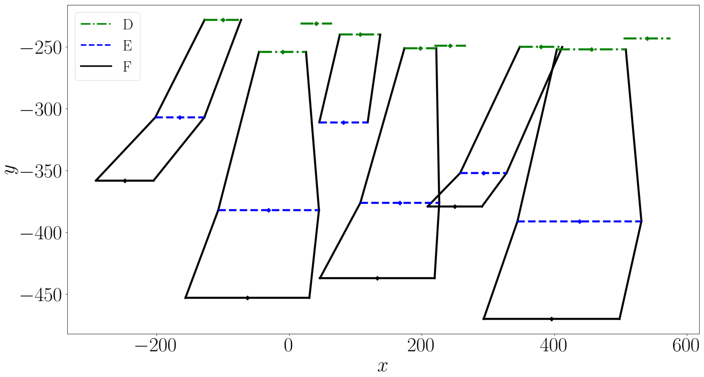
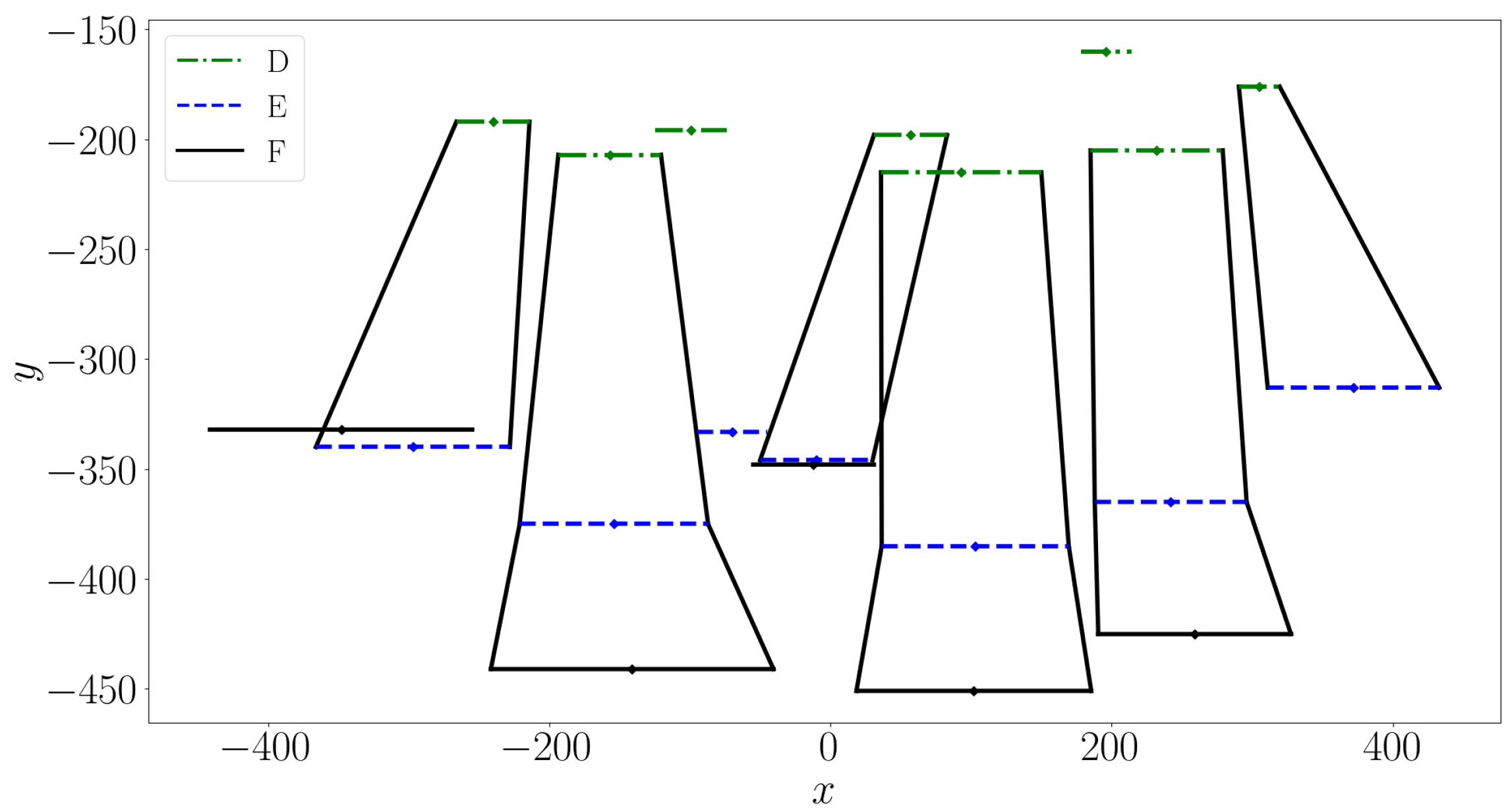
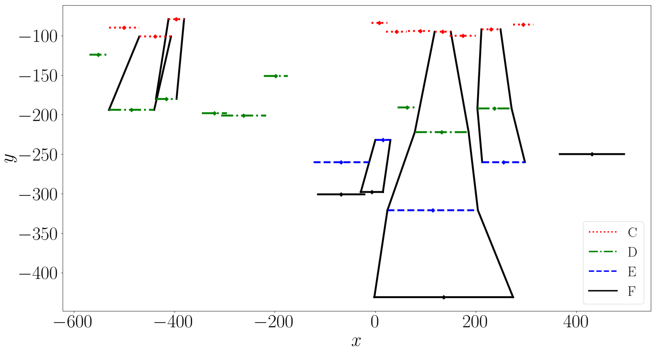
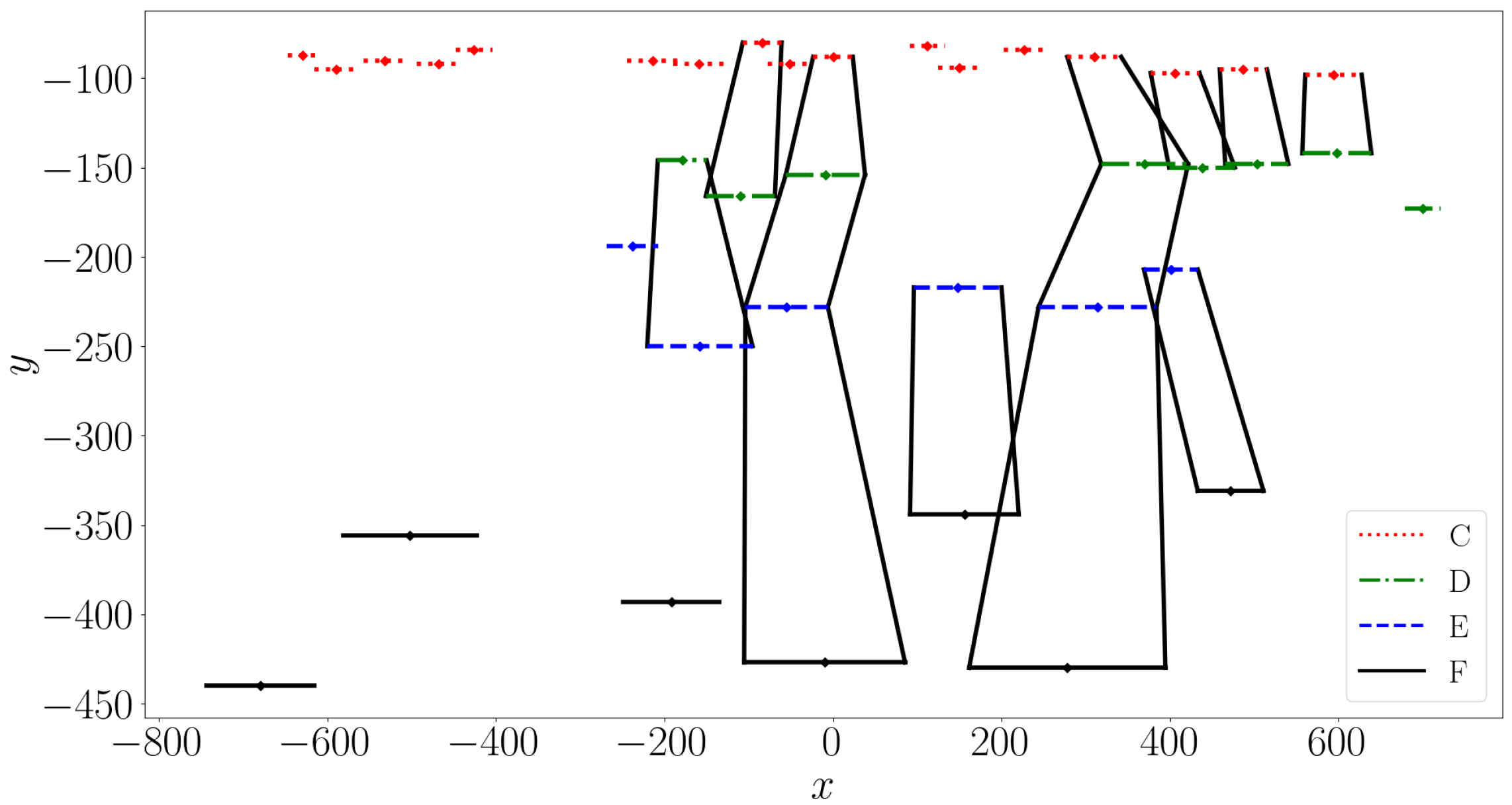
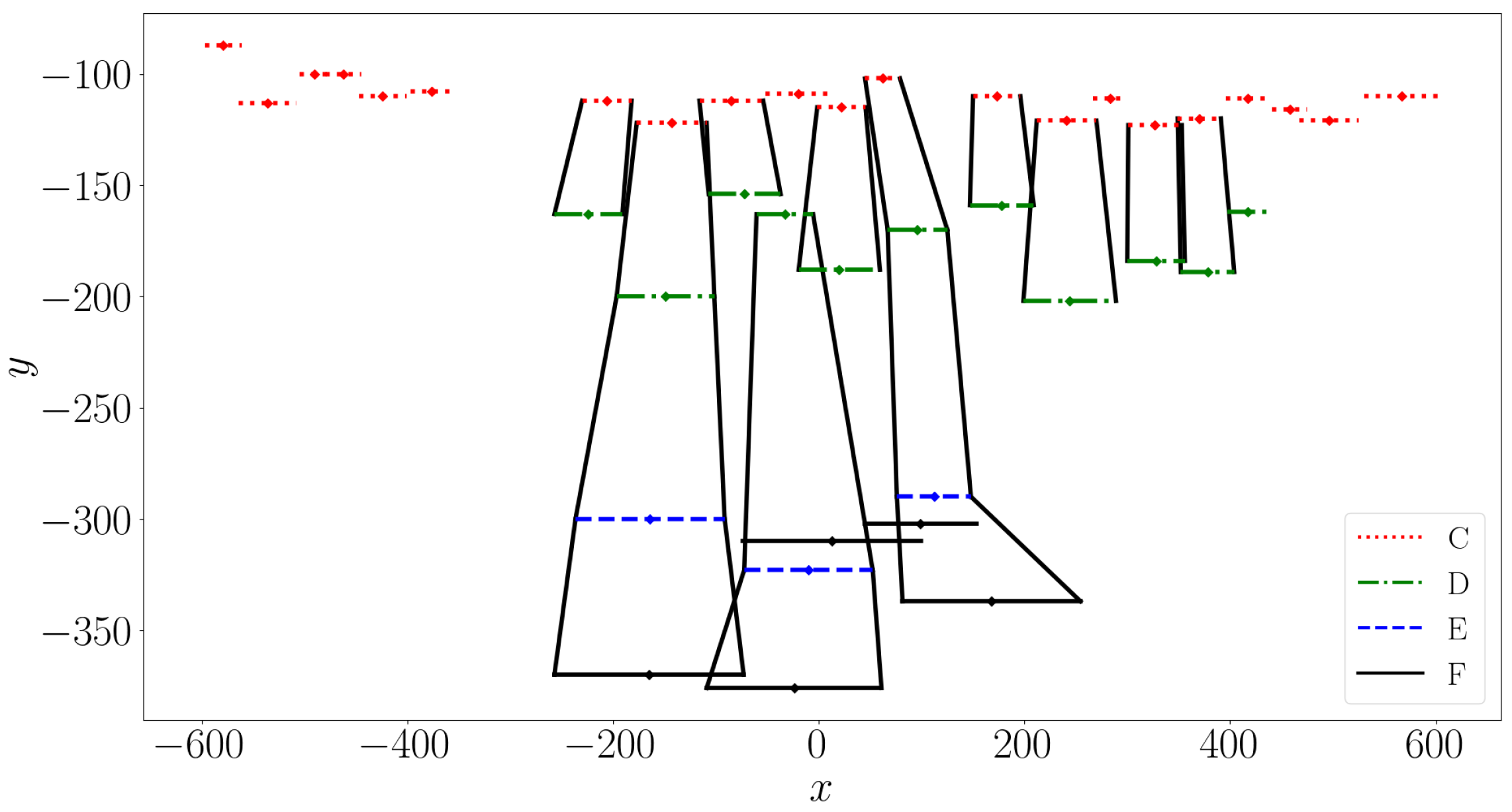
8. 2D Bubble Merger

Five experiments of SY are analyzed (numbered 99, 103, 104, 105, and 114). Plates A-F in each experiment reflect six subsequent times in the evolution of the mixing front. The elapsed time between plates varies by experiment and are shown in Table 1. These experiments are presented as photographs taken from face on cameras, so the resulting data are essentially two-dimensional. The acceleration is tangential to the y-axis in these experiments. The data show a few of the bubbles surviving until the final plate, while many smaller bubbles, present initially, are left behind and disappear from the mixing front and from the plots as time evolves. As the fronts are moving downward in time, the later bubbles are below the earlier ones. We show the larger of the observed bubbles at each time frame. The edges of the same bubble, observed at successive times, are joined to provide a picture of the continuous evolution of each major bubble.
Analysis is omitted for Plates A and B across all experiments due to the low resolution and small amplitudes of bubbles. Plate C is also omitted for Experiments 99 and 103 for identical reasons. Plate photographs are scaled using tank dimensions from SY and center-line values from [54].
To minimize the possibility of interpretation errors in assigning heights and widths to each bubble, both values are independently measured for all bubbles in the ensemble by two authors. Leading bubbles are defined as bubbles with the furthest penetration and with sufficiently large radii. Two authors independently identify the leading bubbles of each plate.
We construct a merger path for a qualitative analysis of the bubble merger using bubble positions and widths. Construction of merger paths begins with the terminal leading bubbles of each experiment and continues working backwards in time to identify its predecessor(s).
Figure 17, Figure 18, Figure 19, Figure 20 and Figure 21 present bubble merger trees, which contain the leading bubbles of each plate along with their adjacent neighbors. For all bubbles in the ensemble, including those not involved in a merger, we represent their widths by a horizontal line. Coloring and line styles are used to identify a bubble’s plate of origin. One can observe the merger process, where a given bubble grows systematically by expanding into space vacated by smaller bubbles. We quantify this observation in Table 2a.

9. 3D Bubble Merger

We construct the three-dimensional analogue of the merger trees found in Section 8. The 3D nature of the data introduces additional difficulties in its analysis and presentation. We examine simulation data modeling the miscible and compressible SY [46], Experiment 112. This experiment involves sodium iodide solution ( ρ h = 1.89 g/cm 3 ) and a solution consisting of water, hydrochloric acid, and phenolphthalein ( ρ l = 1.00 g/cm 3 ), with an approximate Atwood number of 0.3. The mean acceleration is 39 g 0 , where g 0 = 9.81 m/s 2 . The domain in this simulation has dimensions 3.75 cm × 0.625 cm × 15 cm, with periodic boundaries in the x-y plane, and it has no edge effects. The spatial mesh has spacing Δ x = Δ y = Δ z = 5 / 192 , and the numbers of grid cells are N x = 144 , N y = 24 , and N z = 567 . The initial conditions contain short-wavelength perturbations and the equation of state for this simulation is a gamma law gas. We thank Tulin Kaman for providing the simulation data used in this study. For details on a related simulation study of Experiment 112, see [55].
Simulations are analyzed at four time steps (40, 50, 60, and 70 ms), each corresponding to one of the Plates C–F from Experiment 112 of SY [
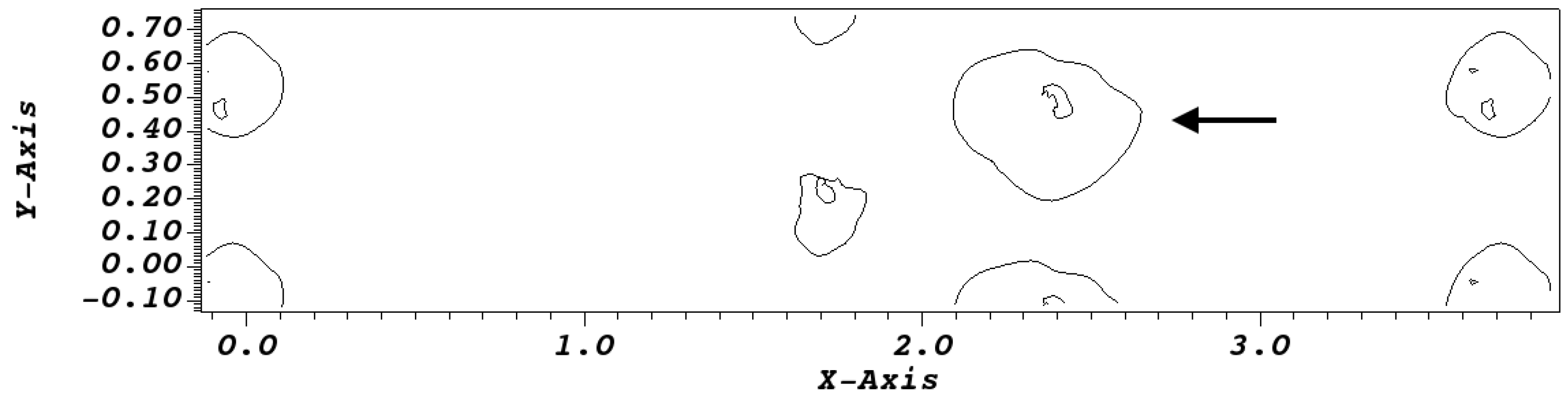
46]. Data from these simulations consist of a meshed interface modeling the mixing front and discrete state variables, namely density. Unlike the 2D case of the preceding section, we note greater ambiguity in identifying bubbles of light fluid in the mixing front. We define a bubble as a structure of reasonable shape that grows from a distinct tip. An example is shown in Figure 22. We observe that in this example, the bubble structure contains a filament of heavy fluid within its enclosure, which we ignore in subsequent analyses.
At a fixed time step, we identify distinct bubble tips and record each bubble’s height at three distinct levels. The lowest height is the bubble tip, above this is a larger cross-section at the middle of the downward moving bubble, and above that is a rim that forms the upper limit of the bubble within the fluid. A bubble’s terminal rim is defined as the largest of the bubble’s heights at which its cross-section has a consistent and maximum shape. The data analysis consists of examination of cross-sections at different height (z) levels through the simulation data.
Following data collection and bubble identification, we construct a merger path for each terminal bubble. That is, for each terminal bubble, we determine what bubble(s) must have preceded it in earlier time steps. The resulting five merger paths are presented in Table 3; here, p is used to denote a bubble split periodically in that respective coordinate. We note in particular Bubble 5 of Table 3, which originates from two distinct tips but terminates at a common base, and so the merger must have occurred at a height beyond the tip.
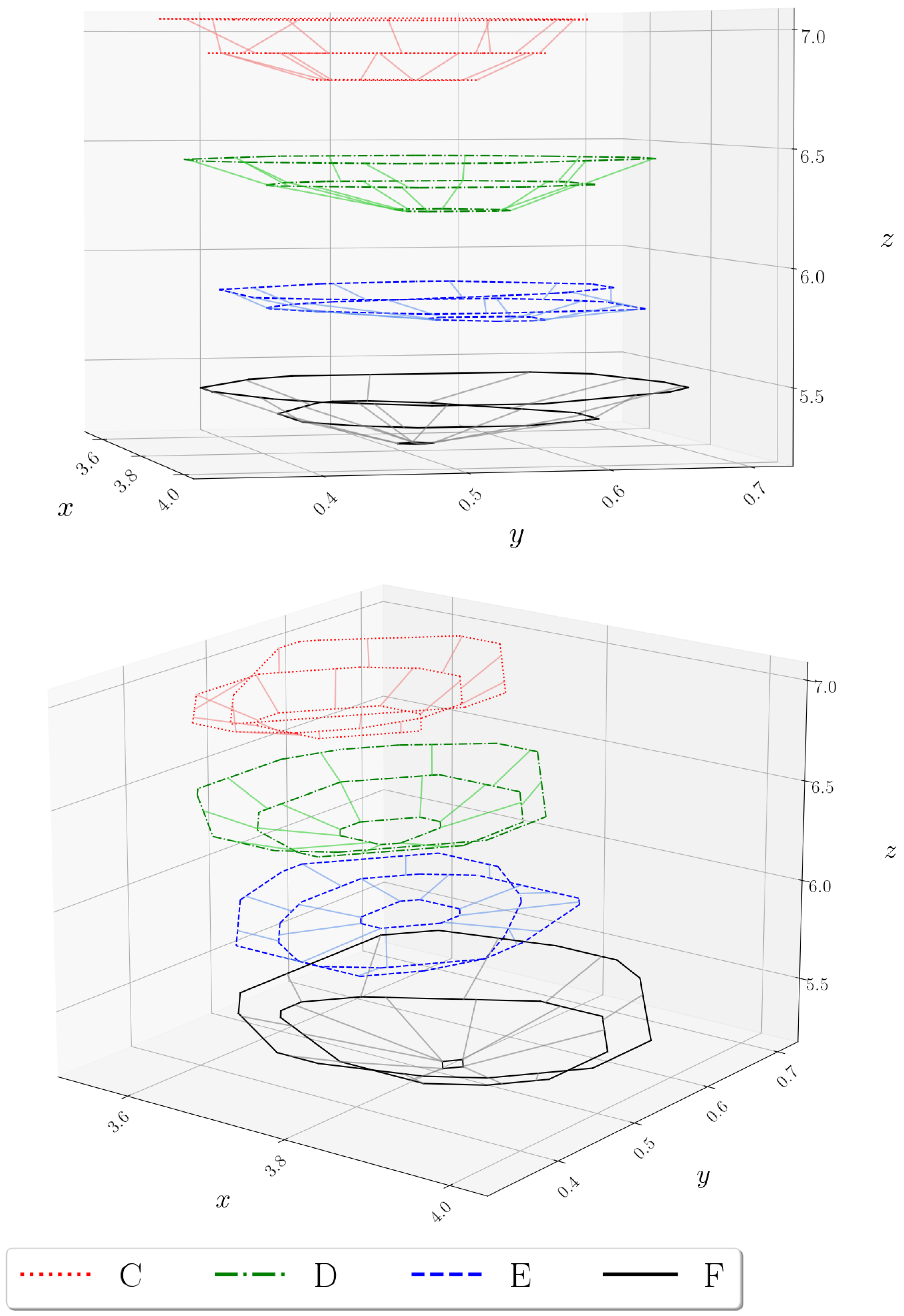
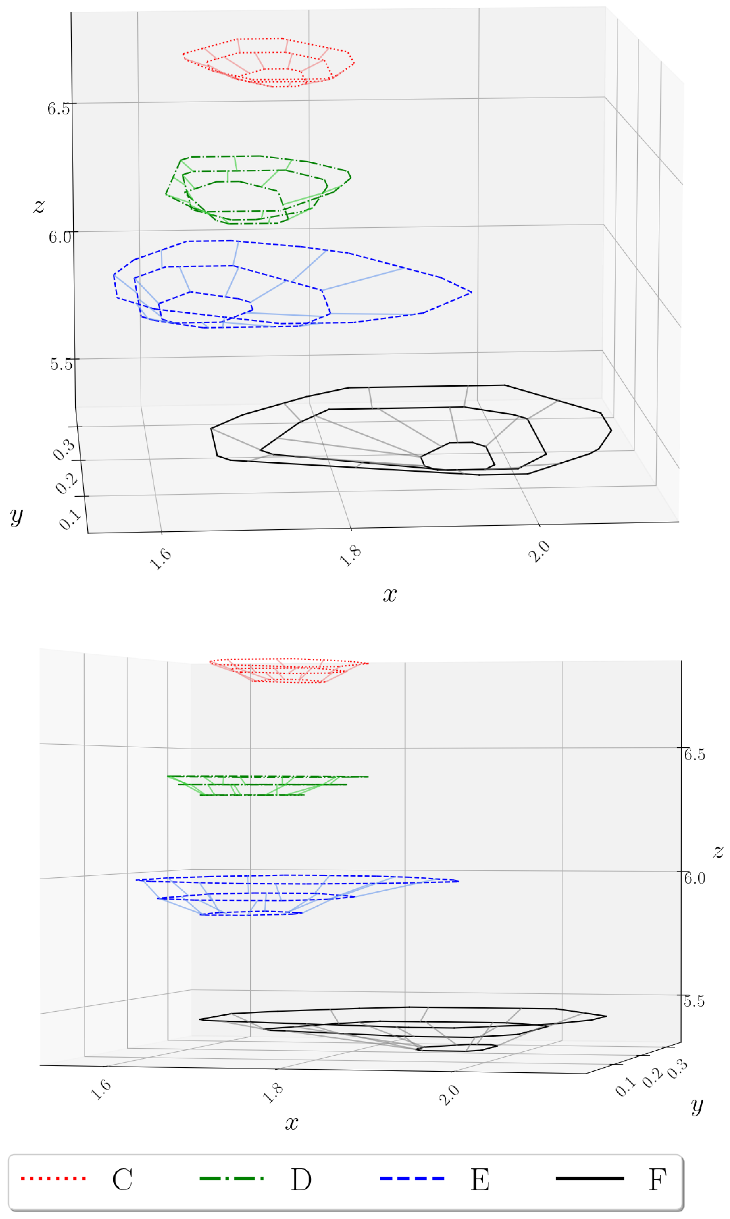
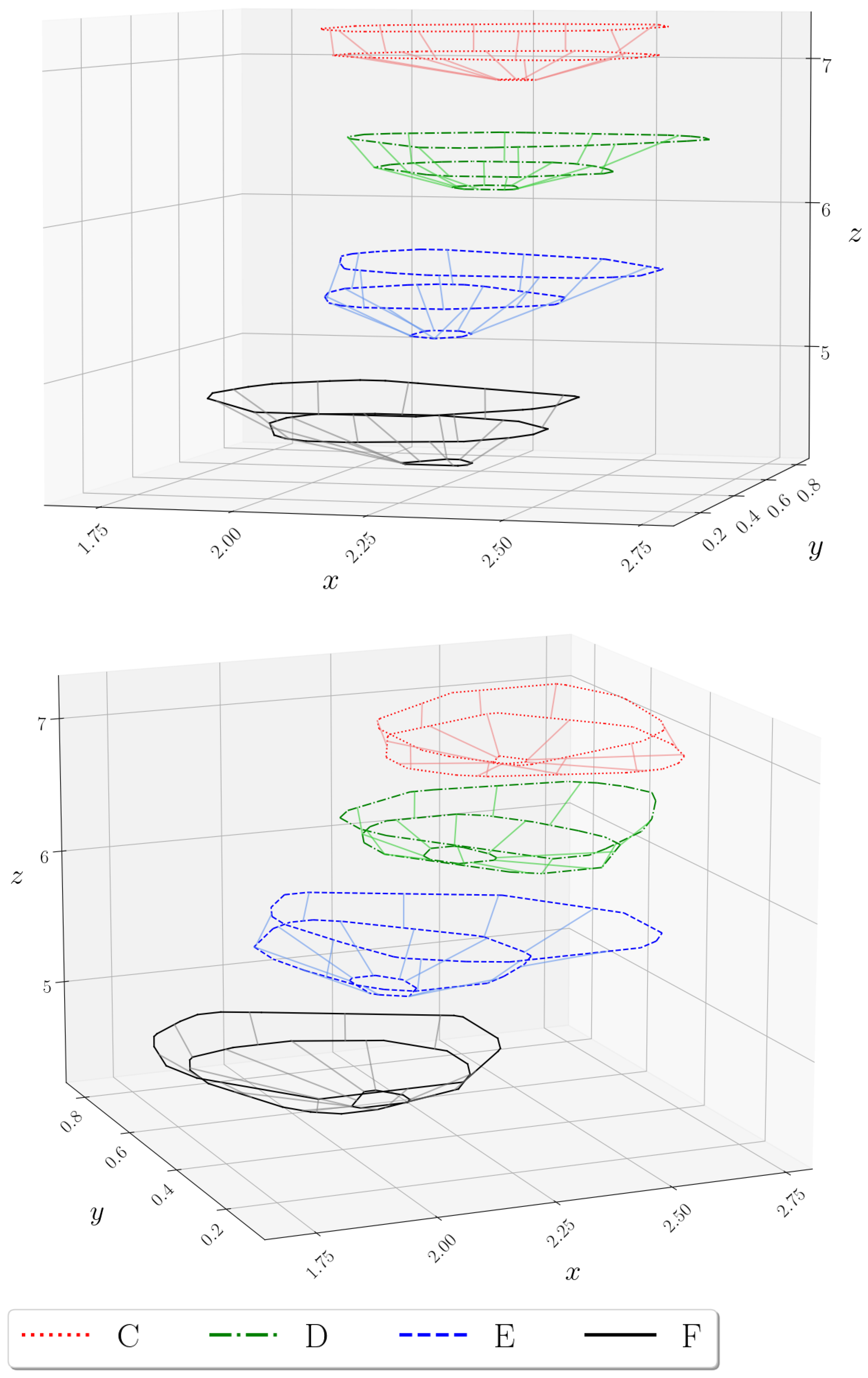
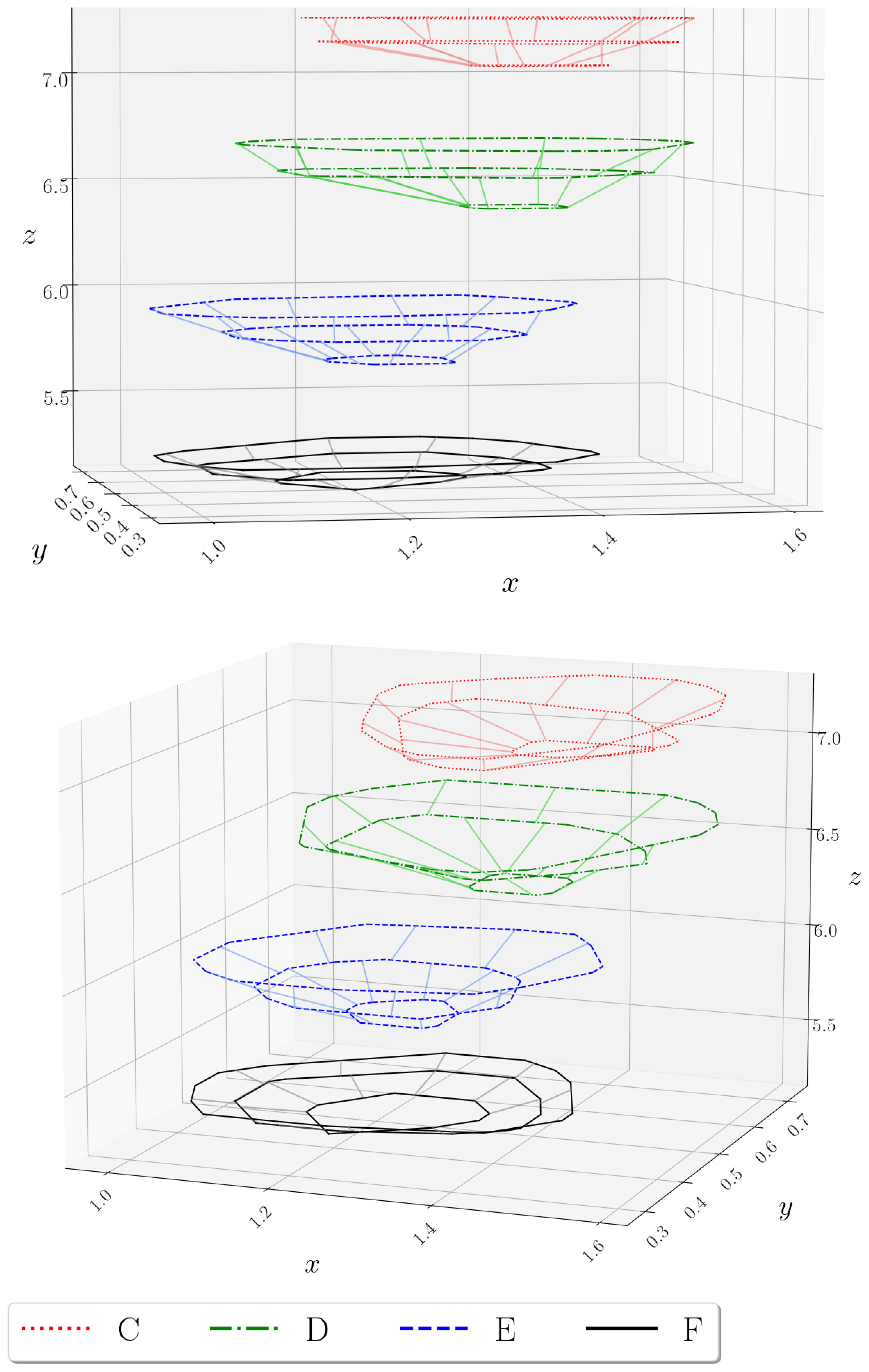
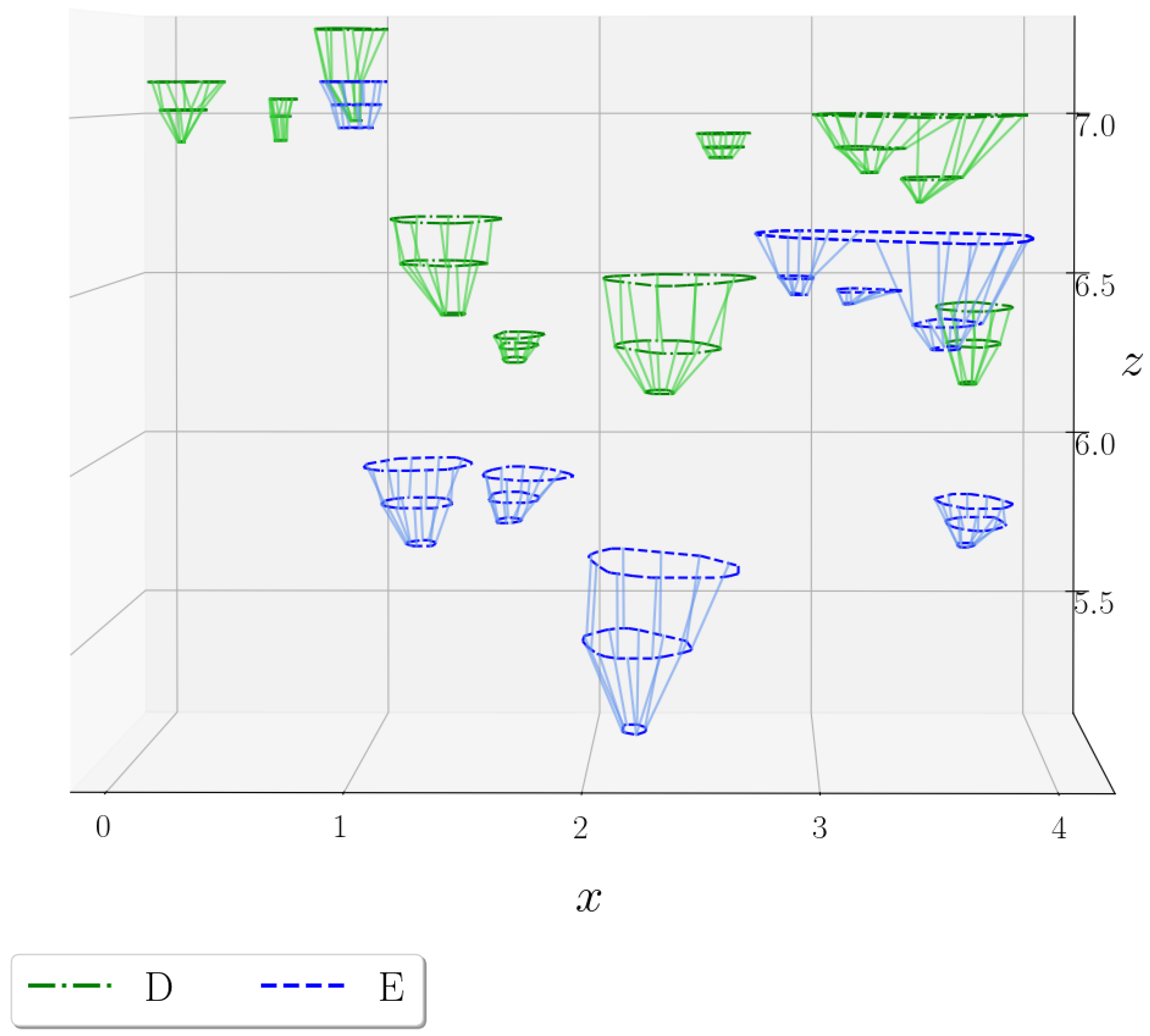
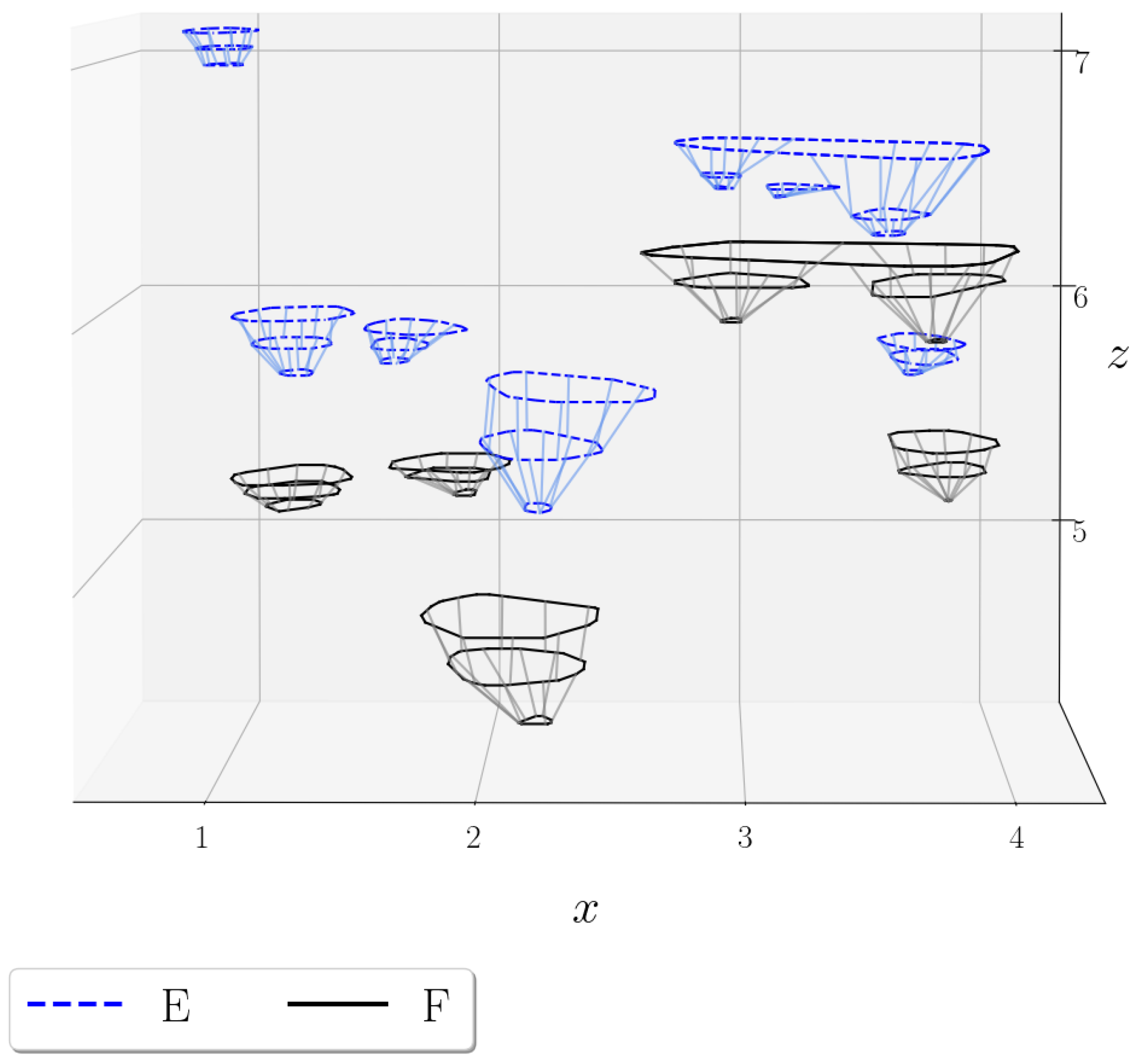
We now outline the process of constructing the 3D merger trees. For a given bubble, we first extract three 2D subsets from the 3D simulation data, one for each of the heights of interest previously discussed. Each slice is digitized, converting all density values to binary values, with each grid block taking a value of zero if it contains density values closer to that of the lighter fluid, and one for values closer to the heavier fluid. A marching squares algorithm, a two-dimensional analogue of the marching cubes algorithm, is then used to identify the vertices of each bubble’s contour. We filter out the non-leading bubbles that do not have the potential to participate as a leading bubble at any time step, using bubble centers to identify the leading bubbles and then take their convex hull. The remaining non-leading bubbles are analyzed separately. Bubbles split by the periodic boundary are reconstructed using appropriate coordinate shifts. Contours are then plotted to create 3D merger trees. Each terminal bubble, and thus each merger tree, is plotted separately. Each bubble is shown at three heights, from the tip to the middle to its base. To suggest time evolution, the bases at the different times are joined by a few nearly vertical line segments. Time evolution is coded by color and line style, consistent with the 2D figures shown in Section 8, with red corresponding to Plate C, green for Plate D, blue for Plate E, and black for Plate F. See Figure 23, Figure 24, Figure 25, Figure 26 and Figure 27, with two alternate viewing angles in most cases.
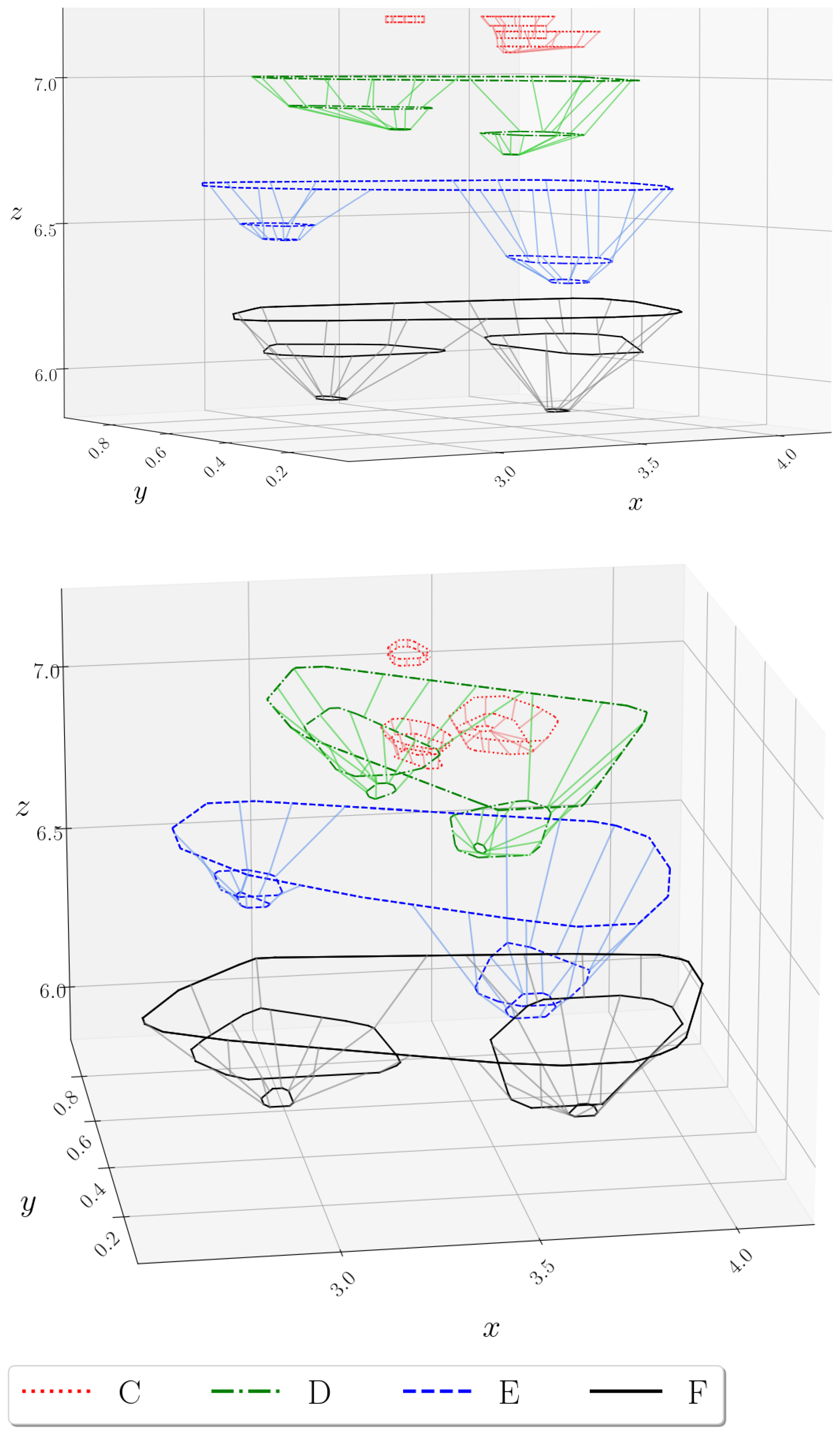
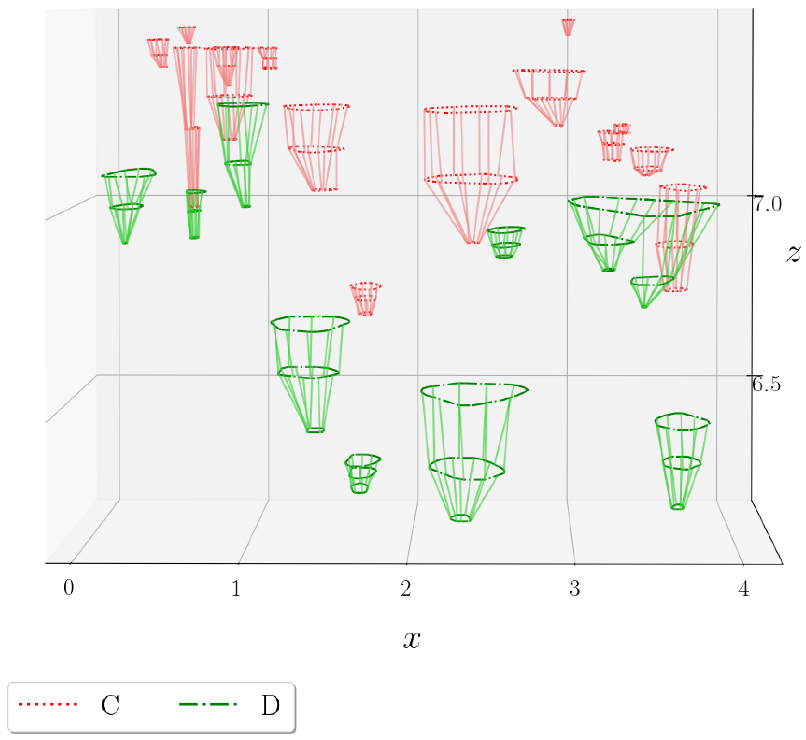
We recall the picture behind the bubble merger model, which states that the larger bubbles expand by occupying space vacated by smaller bubbles that were swept aside. This process can be observed in Figure 28, Figure 29 and Figure 30, where all bubbles in the ensemble, including smaller (non-leading) bubbles, are shown. As in Figure 23, Figure 24, Figure 25, Figure 26 and Figure 27, the time evolution of each bubble is shown using nearly vertical lines connecting three of its cross-sections: the bubble tip, an intermediate height, and the bubble rim. The leading bubbles can be seen expanding with time, and non-leading bubbles are swept aside and ultimately vanish from the mixing front. We quantify these phenomena, both for the 2D and 3D cases, in Table 2b.
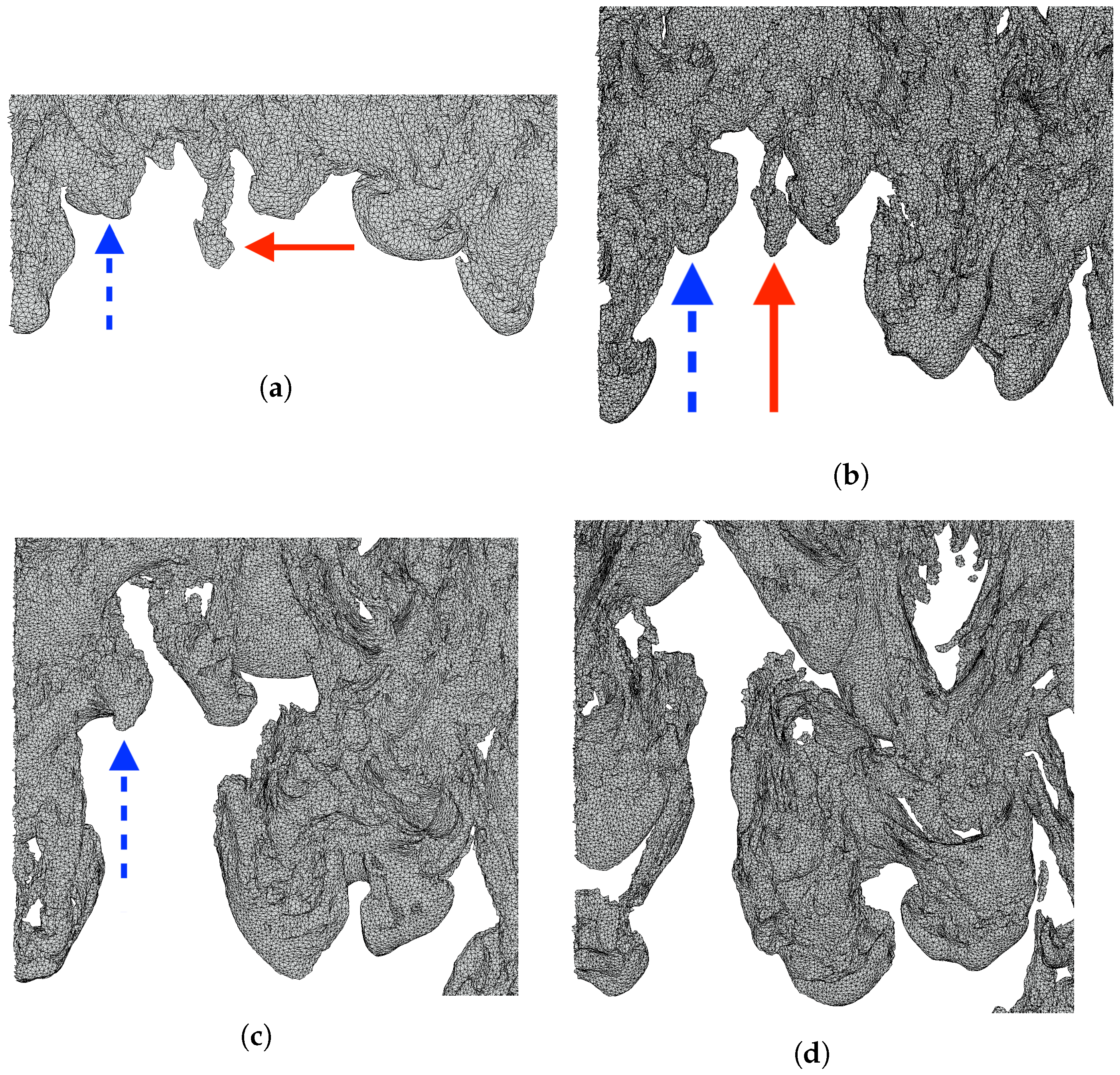
Another example of the bubble merger process can be found in Figure 31. This example follows a fixed region of the mixing front as time evolves. The images in these figures are taken directly from the numerical simulation’s meshed interface data and visualized using the VisIt visualization software. In particular, we point out two smaller, less advanced bubbles, which are indicated by a solid red and dashed blue arrows, respectively. The first bubble survives until Plate D, whereas the second survives until Plate E. By Plate F, we observe that both bubbles have vanished, while the nearby leading bubbles have grown in size and have penetrated further into the heavy fluid.

10. Data Collection and Simulation Growth Rates

We further analyze numerical simulation modeling Experiment 112 discussed in Section 9. In particular, we wish to determine measured values for three growth rate parameters: α b , α r , and α h m . Of most importance is the bubble growth rate, α b , which describes the asymptotic growth behavior of the mixing layer resulting from RT instability [51]. We determine these parameters first by measurement, and later predict these growth rates using the merger model (Section 11 and Section 12). Values for the measured parameters presented in this section can be found in Table 8.
Required quantities are measured using interface data, as opposed to state variables, due to their superior resolution. An example of these interface data is pictured in Figure 31 using the VisIt visualization software.

10.1. Bubble Growth Rate, α b

We recall from Equation (22) that the penetration distance of the bubble front follows a t 2 scaling law. The leading bubble of each time step is defined as the bubble which penetrates furthest into the heavy fluid. The penetration of the leading bubble is taken as the overall penetration distance of the bubble ensemble, and is what we define as h b . Penetration distances for the numerical simulation are provided by Tulin Kaman and are presented in Table 4.
The values for h b are then regressed against scaled acceleration distances X = A g t 2 to determine α b ; see Figure 32. We observe α b = 0.056 in the numerical experiment. The nonzero intercept in Figure 32 suggests a delay in mixing, which is consistent with the original SY experiment.
SY report α b = 0.052 for Experiment 112 [46]. We compare our measured value to SY, but do not expect and do not achieve exact agreement due to the 3.5 mm initial thickness present in the SY experiments, which is in contrast to the sharp interface of the numerical simulation. The role of this initial thickness parameter was studied in [55], and the discrepancy of the simulation α b to the SY value is consistent with study [55].

10.2. Radius Growth Rate, α r

It was shown in [45] that the mean bubble radius, r ¯ , satisfies a self-similar scaling law similar to Equation (22):
r ¯ α r A g t 2 .
We now determine the radius growth rate, α r , for numerical simulation data. We note that the transition from 2D to 3D introduces additional difficulties; in particular, the base of the bubble is not perfectly circular, but rather (approximately) elliptical. Thus, to have a well-defined notion of a bubble’s radius, we define the radius at the base to be half the length of its major axis. We collect radius values for all bubbles in the ensemble, including smaller non-leading bubbles. The mean radius of each plate is presented in Table 5.
By regressing the values of Table 5 against the scaled acceleration distances, we obtain α r = 0.004 ; see Figure 33. The results from Table 5 are consistent with the qualitative picture behind the bubble merger, where bubbles are expanding as time evolves.

10.3. Separation Height Growth Rate, α h m

Another parameter within the merger model is the maximum separation height between adjacent bubbles undergoing a merger, denoted as h m . According to [45], this parameter is also governed by a t 2 scaling law:
h m = α h m A g t 2 .
This can be seen in Figure 31, where the height between adjacent bubbles increases as time evolves.
We wish to determine the growth rate parameter, α h m , for numerical simulation data. To this end, we record the maximum separation distance of adjacent bubbles for each plate. The results are presented in Table 6. As before, the growth rate, α h m , is determined through regression; see Figure 34. We measure α h m = 0.0323 .

11. Review of Merger Model

Here, we present a brief overview of the model and model equations; we refer the reader to [45] for details. The merger model predicts three measured parameters:
1.
the mixing rate, α b ,
2.
the bubble height separation at the time of merger, h m ,
3.
the mean bubble radius, r ¯ ,
and
takes in a noise level as an adjustable input.
This noise level, as presented in the original merger model, is taken to be the variance of the fluctuations amongst bubble radii. More explicitly, for fixed time, the randomness within the bubble ensemble can be measured by first applying map r ( r / r ¯ 1 ), where r is the bubble radius, and computing the variance of the transformed distribution. Area preservation and geometrical arguments concerning bubble merger lead to defining parameter
k r new r 1 + r 2 2 / r 1 + r 2 2 ,
where
r 1 = r ¯ ( 1 + σ ) , r 2 = r ¯ ( 1 σ ) , r new = r 1 2 + r 2 2 ,
and σ is the standard deviation of fluctuations amongst bubble radii. After some elementary manipulations, Equation (25) can be rewritten to be independent of r ¯ :
k = 2 ( 1 + σ 2 ) 1 .
We recall that h m and r ¯ satisfy self-similar scaling laws:
r ¯ ( t ) α r A g t 2 , α r = k 2 1 t m * 2 ,
and
h m = α h m A g t 2 , α h m = k 2 4 h m 1 t m * 2 = h m α r ,
where h m = h m / r ¯ , and 1 / t m * is the averaged merger rate evaluated at the renormalization group fixed point.
Using the above, the model predicts α b as
α b = k 4 c b + 1 + k 2 h m 1 t m * 1 t m * = 1 2 c b α r 1 / 2 + 1 2 k + 1 2 α h m ,
where c b is a constant obtained from experiment or from theoretical determination. In all subsequent analyses, we follow [45] and take c b = 0.532 for hexagonal bubbles.
Thus, given a measure of randomness, a prediction for α b using Equation (29) reduces to determining h m and 1 / t m * . To this end, we consider two interacting adjacent bubbles with radii r 1 and r 2 . We let r l = min ( r 1 , r 2 ) and r h = max ( r 1 , r 2 ) . We note that ratio r h / r l is then itself a measure of randomness. When using experimental data, this value can be computed directly from the standard deviation of bubble radii using
r h r l = r ¯ ( 1 + σ ) r ¯ ( 1 σ ) = 1 + σ 1 σ .
The velocity of a single bubble, when used in conjunction with geometric considerations of interacting bubble tips on a larger length scale, provides a criterion for completion of merger:
6 χ 1 / 2 = 5 λ 1 / 2 e λ x m / 2 λ x m / 2 1 e λ x m / 2 + 1 1 / 2 + e x m x m 1 e x m + 1 1 / 2 ,
where
R r h + r l
x m h m β 1 / R
χ 1 + r h / r l
λ χ 1 + 1 + ( χ 1 ) 2 / 2 ,
and β 1 is the first zero of the Bessel function, J 1 ( r ) .
We observe that solving Equation (31) for x m and using Equation (33), along with the fact that R / r ¯ = ( r h + r l ) / [ ( r h + r l ) / 2 ] = 2 , yields h m , as desired.
The model determines 1 / t m * by using the already found value for x m :
1 t m * = 1 x m 2 0 x m x m x t m ( x ) d x ,
where
t m 3 2 β 1 x x m e x x 1 e x + 1 + 5 λ e λ x / 2 λ x / 2 1 e λ x / 2 + 1 1 d x .
Having determined the averaged merger rate at the RNG fixed point, we may use Equations (27)–(29) to predict theoretically the growth rates, α r , α h m , and α b .

12. Application of Model to Experiment

We use the process outlined in Section 11 to predict model parameters. We begin first by applying the model to various radius ratios r h / r l and reproduce Table III of [45] keeping all notation consistent; the results are shown in Table 7. We then apply the model to Experiments 104, 105, and 114 of SY, and compare the results with those reported in [45]. We present these predictions in Table 8. For consistency, we use the measured standard deviation reported in [45] as an input into the model.
Minor discrepancies in the numerical solution for nonlinear Equation (31) are corrected, as well as the modifications to the experimental predictions. α b prediction improves in comparison to the experiment, while predictions for α r and α h m become somewhat worse. These changes are made with the acceptance of the authors of [45].
Additionally, we apply the model to the 3D numerical simulation modeling Experiment 112 of SY that is discussed in Section 9 and Section 10. We measure the radius at the base of each bubble in the ensemble and measure the fluctuations within the resulting distribution as was discussed in Section 11, similar to the 2D analysis carried out in [45]. Due to the 3D nature of the simulation, the cross-sections at the base are not perfectly circular and so we note some ambiguity in interpreting its radius. We map these standard deviations to radius ratios using Equation (30) as input to the model. The results can be found in the last row of Table 8.
We recall from Section 10.1 that we cannot confirm that the sharp interface in the numerical simulations is relevant to SY’s Experiment 112 [46]. Furthermore, the unavailability of data from earlier time steps renders our application of the merger model to simulation incomplete. We posit that this exclusion has an influence on the predicted value for α b . For these reasons, we do not compare the merger model prediction to the α b value measured in either experiment or simulation.

13. Outcomes

We studied RTI driven by constant acceleration in neutral plasmas (fluids and/or gases). We employed the group theory analytical approach and the analysis of numerical data in Front Tracking simulations. We revealed the independent driving constituents that RT flow possesses in each of the linear, nonlinear, and mixing regimes.

13.1. Outcomes from Analysis

In our analysis, we employed the group theory approach and directly linked the governing equations to the dynamical system and the momentum model [4,38]. We precisely derived the buoyancy and drag parameters for RT bubbles and RT spikes in the linear, nonlinear, and mixing regimes. The governing equations include the conservation laws in the bulk, the boundary value problem at the interface and the initial value problem; see Equations (1), (2) and (6). They are reduced to the dynamical system by using an irreducible representation of the group of RT flow. The momentum model has the same symmetries and scaling transformations as the governing equations; see Equations (3)–(7).
In each regime, we precisely derived from the governing equations the momentum model parameters for RT bubbles and RT spikes. We integrated the momentum model equations and investigated their asymptotic limits, finding complete consistency with asymptotic analytical solutions for the dynamical system; see Equations (8) and (9) and Figure 3, Figure 4, Figure 5 and Figure 6. In addition to the interplay of harmonics, the group theory approach captures the interfacial character of RT dynamics, with intense fluid motion at the interface, effectively no motion far from the interface, and with shear-driven vortical structure at the interface; see works [13,38]. Our approach can be applied to three-dimensional and two-dimensional RT flows [4].
We revealed that the buoyancy and drag parameters are independent characteristics of RT dynamics. The expressions for the buoyancy and drag parameters are distinct in the early-time linear, later-time nonlinear, and mixing regimes. They are also distinct for RT bubbles and RT spikes. In addition to the density ratio, they depend on the interface morphology and the interfacial shear. However, they are independent of the acceleration, thus expanding the validity of our results to variable, in space and time, accelerations; see Equations (8)–(10) and (21) and Figure 1, Figure 2 and Figure 7, Figure 8, Figure 9, Figure 10, Figure 11, Figure 12, Figure 13, Figure 14, Figure 15 and Figure 16.

13.2. Outcomes from Simulations

In regard to simulations, we presented 2D and 3D merger tree diagrams showing the dynamics of the merger model. In these figures, we observed that smaller and less advanced bubbles are pushed downstream and away from the mixing front. Larger and leading bubbles expand into this vacated space. Hence, we concluded that the qualitative picture behind the bubble merger is correct. Figures showing the growth of a single bubble as a result of this process are also presented, including an incomplete merger with two distinct tips merging to a common base; see Figure 17, Figure 18, Figure 19, Figure 20 and Figure 21 and Figure 23, Figure 24, Figure 25, Figure 26, Figure 27, Figure 28, Figure 29, Figure 30 and Figure 31.
We analyzed numerical simulation data modeling Experiment 112 of SY and presented a detailed data analysis; see Section 10. Due to the significant difference in the initial thickness of the mixing layer in the SY experiment (3.5 mm) and the numerical simulation (0 mm), we did not compare our parameter values to the SY data.
On the quantitative side, we revisited predictions made by the merger model [45] and corrected the numerical solution to a nonlinear equation pertaining to the model. The result is an improvement in α b for all three experiments, and some worsening of the two other growth rate parameters α r and α h m . We applied this model to the numerical simulation data and presented similar findings; we predicted α b = 0.067 . We did not compare this prediction to the value measured in experiment or simulation due to the absence of early time data; see Table 7 and Table 8.
The success of this model indicates that the direct measurement of randomness related to the bubble front evolution, in terms of a measured variance and standard deviation, is feasible both for simulation data and data collected from physical (2D) experiments. The results of this analysis may motivate future studies of bubble merger to further investigate the growth of randomness in hopes of constructing a fully theoretical model.

13.3. Outcomes for Plasma Experiments

Our analysis and simulations suggests the following implications in our considerations for plasma experiments, including inertial confinement fusion [9,34,36]. (1) RT dynamics are driven by two independent constituents—the buoyancy and the drag. The values of the buoyancy and drag parameters depend on the regime and on the deterministic conditions, and are distinct for bubbles and spikes; see Equations (8), (10) and (21) and Figure 1, Figure 2 and Figure 7, Figure 8, Figure 9, Figure 10, Figure 11, Figure 12, Figure 13, Figure 14, Figure 15 and Figure 16. (2) In order to accurately describe experimental and numerical simulation data for uncontrolled broadband initial conditions, one needs to consider two independent self-similar processes—the merger process, as introduced in Section 1, and the amplitude growth process; see Equations (8), (9) and (21) and Figure 1 and Figure 2. (3) RT dynamics can, in principle, be controlled, by means of the deterministic conditions (i.e., the initial and the flow experimental conditions), in agreement with experiments in fluids and plasmas at high Reynolds numbers [13,38].
Our results suggest new opportunities for control of plasma flows by means of these deterministic conditions [9,33,34,36]. For instance, in inertial confinement fusion (ICF), it may be worth scratching the target in order to impose proper deterministic conditions and to gain better control of fluid instabilities and the interfacial mixing. This may help existing methods focused on fine polishing of ICF targets in order to fully eliminate RTI [9]. Our results can also be applied in nanofabrication, by describing the dynamics and morphology of the RT unstable interface in the scale-dependent linear and nonlinear regimes, and their scaling properties, along with the sensitivity to deterministic conditions in the self-similar mixing regime [26].

14. Conclusions

We studied, analytically and numerically, RTI with constant acceleration in neutral plasma (fluid) by employing the group theory approach and the merger model. Based on the obtained analytical solutions and conclusions drawn from the data analysis of numerical and physical experiments, we revealed the independent constituents governing RT dynamics in the linear, nonlinear, and mixing regimes. Our results can be used to enhance methods of control of RT unstable plasma flows.

Author Contributions

The authors contributed to this work as follows. Conceptualization, J.G. and S.A.; Methodology, J.G. and S.A.; Formal analysis, D.H., J.G. and S.A.; Validation, A.H.R.; Investigation, A.H.R. and D.H.; Data curation. A.H.R.; Visualization, A.H.R. and D.H.; Writing–original draft, A.H.R., D.H., J.G. and S.A.; Writing–revision, A.H.R., J.G. and S.A.; Supervision, J.G. and S.A. Numerical simulations, A.H.R. and J.G. Theory, D.H. and S.A. All authors have read and agreed to the published version of the manuscript.

Funding

This research received no external funding.

Data Availability Statement

The data presented in this study are available on request from the corresponding author.

Conflicts of Interest

The authors declare no conflict of interest.

References

  1. Rayleigh, L. Investigations of the character of the equilibrium of an incompressible heavy fluid of variable density. Proc. Lond. Math. Soc. 1883, 14, 170–177. [Google Scholar] [CrossRef]
  2. Taylor, G. The formation of a blast wave by a very intense explosion.—II. The atomic explosion of 1945. Proc. R. Soc. Lond. 1950, 201, 175–186. [Google Scholar] [CrossRef]
  3. Davies, R.; Taylor, G. The mechanics of large bubbles rising through extended liquids and through liquids in tubes. Proc. R. Soc. Lond. Ser. A Math. Phys. Sci. 1950, 200, 375–390. [Google Scholar] [CrossRef]
  4. Abarzhi, S. Review of theoretical modelling approaches of Rayleigh-Taylor instabilities and turbulent mixing. Philos. Trans. R. Soc. A Math. Phys. Eng. Sci. 2010, 368, 1809–1828. [Google Scholar] [CrossRef] [PubMed]
  5. Glimm, J.; Sharp, D. Chaotic mixing as a renormalisation-group fixed point. Phys. Rev. Lett. 1990, 64, 2137–2139. [Google Scholar] [CrossRef] [PubMed]
  6. Meshkov, E. Some peculiar features of hydrodynamic instability development. Philos. Trans. R. Soc. A Math. Phys. Eng. Sci. 2013, 371, 20120288. [Google Scholar] [CrossRef]
  7. Arnett, W.D. Supernovae and Nucleosynthesis: An Investigation of the History of Matter, from the Big Bang to the Present; Princeton Series in Astrophysics; Princeton University Press: Princeton, NJ, USA, 1996. [Google Scholar]
  8. Buehler, M.; Tang, H.; van Duin, A.; Goddard, W. Threshold Crack Speed Controls Dynamical Fracture of Silicon Single Crystals. Phys. Rev. Lett. 2007, 99, 165502. [Google Scholar] [CrossRef]
  9. Haan, S.W.; Lindl, J.D.; Callahan, D.A.; Clark, D.S.; Salmonson, J.D.; Hammel, B.A.; Atherton, L.J.; Cook, R.C.; Edwards, M.J.; Glenzer, S.; et al. Point design targets, specifications, and requirements for the 2010 ignition campaign on the National Ignition Facility. Phys. Plasmas 2011, 18, 051001. [Google Scholar] [CrossRef]
  10. Azechi, H.; Sakaiya, T.; Fujioka, S.; Tamari, Y.; Otani, K.; Shigemori, K.; Nakai, M.; Shiraga, H.; Miyanaga, N.; Mima, K. Comprehensive diagnosis of growth rates of the ablative Rayleigh-Taylor instability. Phys. Rev. Lett. 2007, 98, 045002. [Google Scholar] [CrossRef]
  11. Drake, R.P. Perspectives on high-energy-density physics. Phys. Plasmas 2009, 16, 055501. [Google Scholar] [CrossRef]
  12. Underwood, T.C.; Loebner, K.T.; Miller, V.A.; Cappelli, M.A. Dynamic formation of stable current-driven plasma jets. Sci. Rep. 2019, 9, 2588. [Google Scholar] [CrossRef] [PubMed]
  13. Abarzhi, S.; Bhowmick, A.; Naveh, A.; Pandian, A.; Swisher, N.; Stellingwerf, R.; Arnett, W. Supernova, nuclear synthesis, fluid instabilities, and interfacial mixing. Proc. Natl. Acad. Sci. USA 2019, 116, 18184–18192. [Google Scholar] [CrossRef] [PubMed]
  14. Kuranz, C.C.; Park, H.S.; Huntington, C.M.; Miles, A.R.; Remington, B.A.; Plewa, T.; Trantham, M.; Robey, H.; Shvarts, D.; Shimony, A.; et al. How high energy fluxes may affect Rayleigh–Taylor instability growth in young supernova remnants. Nat. Commun. 2018, 9, 1564. [Google Scholar] [CrossRef] [PubMed]
  15. Rigon, G.; Albertazzi, B.; Pikuz, T.; Mabey, P.; Bouffetier, V.; Ozaki, N.; Vinci, T.; Barbato, F.; Falize, E.; Inubushi, Y.; et al. Micron-scale phenomena observed in a turbulent laser-produced plasma. Nat. Commun. 2021, 12, 2679. [Google Scholar] [CrossRef] [PubMed]
  16. Remington, B.A.; Drake, R.P.; Takabe, H.; Arnett, D. A review of astrophysics experiments on intense lasers. Phys. Plasmas 2000, 7, 1641–1652. [Google Scholar] [CrossRef]
  17. Robey, H. Effects of viscosity and mass diffusion in hydrodynamically unstable plasma flows. Phys. Plasmas 2004, 11, 4123–4133. [Google Scholar] [CrossRef]
  18. Stein, R.; Norlund, A. Realistic solar convection simulations. Sol. Phys. 2000, 192, 91–108. [Google Scholar] [CrossRef]
  19. Lindl, J. Development of the indirect-drive approach to inertial confinement fusion and the target physics basis for ignition and gain. Phys. Plasmas 1995, 2, 3933–4024. [Google Scholar] [CrossRef]
  20. Smalyuk, V.; Hu, S.; Goncharov, V.; Meyerhofer, D.; Sangster, T.; Stoeckl, C.; Yaakobi, B. Systematic study of Rayleigh–Taylor growth in directly driven plastic targets in a laser-intensity range from 2 × 10¹⁴ to 1.5 × 10¹⁵ W/ cm2. Phys. Plasmas 2008, 15, 082703. [Google Scholar] [CrossRef]
  21. Casner, A.; Mailliet, C.; Khan, S.; Martinez, D.; Izumi, N.; Kalantar, D.; Di Nicola, P.; Di Nicola, J.; Le Bel, E.; Igumenshchev, I.; et al. Long-duration planar direct-drive hydrodynamics experiments on the NIF. Plasma Phys. Control. Fusion 2017, 60, 014012. [Google Scholar] [CrossRef]
  22. Remington, B.; Park, H.S.; Casey, D.; Cavallo, R.; Clark, D.; Huntington, C.; Kuranz, C.; Miles, A.; Nagel, S.; Raman, K.; et al. Rayleigh-Taylor instabilities in high-energy density settings on the National Ignition Facility. Proc. Natl. Acad. Sci. USA 2019, 116, 18223–18228. [Google Scholar] [CrossRef] [PubMed]
  23. Matsuo, K.; Sano, T.; Ishigure, K.; Kato, H.; Nagamatsu, N.; Baojun, Z.; Shuwang, G.; Nagatomo, H.; Philippe, N.; Sakawa, Y.; et al. Flash X-ray backlight technique using a Fresnel phase zone plate for measuring interfacial instability. High Energy Density Phys. 2020, 36, 100837. [Google Scholar] [CrossRef]
  24. Schlossberg, D.; Grim, G.; Casey, D.; Moore, A.; Nora, R.; Bachmann, B.; Benedetti, L.; Bionta, R.; Eckart, M.; Field, J.; et al. Observation of hydrodynamic flows in imploding fusion plasmas on the national ignition facility. Phys. Rev. Lett. 2021, 127, 125001. [Google Scholar] [CrossRef] [PubMed]
  25. Mahalov, A.; McDaniel, A. Long-range propagation through inhomogeneous turbulent atmosphere: Analysis beyond phase screens. Phys. Scr. 2019, 94, 034003. [Google Scholar] [CrossRef]
  26. Zhakhovsky, V.; Kryukov, A.; Levashov, V.; Shishkov, I.; Anisimov, S. Mass and heat transfer between evaporation and condensation surfaces: Atomistic simulation and solution of Boltzmann kinetic equation. Proc. Natl. Acad. Sci. USA 2019, 116, 18209–18217. [Google Scholar] [CrossRef] [PubMed]
  27. Lugomer, S. Laser-generated Richtmyer–Meshkov and Rayleigh–Taylor instabilities. III. Nearperipheral region of Gaussian spot. Laser Part. Beams 2016, 35, 597–609. [Google Scholar] [CrossRef]
  28. Lugomer, S. Laser-generated Richtmyer–Meshkov and Rayleigh–Taylor instabilities in a semiconfined configuration: Bubble dynamics in the central region of the Gaussian spot. Phys. Scr. 2018, 94, 015001. [Google Scholar] [CrossRef]
  29. Kaneko, T.; Baba, K.; Hatakeyama, R. Static gas–liquid interfacial direct current discharge plasmas using ionic liquid cathode. J. Appl. Phys. 2009, 105, 103306. [Google Scholar] [CrossRef]
  30. Chandrasekhar, S. Hydrodynamic and Hydromagnetic Stability; Oxford University Press: Oxford, UK, 1961. [Google Scholar]
  31. Kadau, K.; Barber, J.; Germann, T.; Holian, B.; Alder, B. Atomistic methods in fluid simulation. Phil. Trans. R Soc. A 2010, 368, 1547. [Google Scholar] [CrossRef]
  32. Landau, L.; Lifshitz, E. Course of Theoretical Physics; Elsevier Science: Amsterdam, The Netherlands, 1987; Volume I–X. [Google Scholar]
  33. Abarzhi, S. Self-similar interfacial mixing with variable acceleration. Phys. Fluids 2021, 33, 122110. [Google Scholar] [CrossRef]
  34. Robey, H.; Zhou, Y.; Buckingham, A.; Keiter, P.; Remington, B.; Drake, R. The time scale for the transition to turbulence in a high Reynolds number, accelerated flow. Phys. Plasmas 2003, 10, 614. [Google Scholar] [CrossRef]
  35. Youngs, D. The density ratio dependence of self-similar Rayleigh-Taylor mixing. Phil. Trans. R. Soc. A 2013, 371, 20120173. [Google Scholar] [CrossRef] [PubMed]
  36. Swisher, N.; Kuranz, C.C.; Arnett, D.; Hurricane, O.; Remington, B.A.; Robey, H.F.; Abarzhi, S.I. Rayleigh-Taylor mixing in supernova experiments. Phys. Plasmas 2015, 22, 102707. [Google Scholar] [CrossRef]
  37. Alon, U.; Hecht, J.; Ofer, D.; Shvarts, D. Power Laws and Similarity of Rayleigh-Taylor and Richtmyer-Meshkov Mixing Fronts at all Density Ratios. Phys. Rev. Lett. 1995, 74, 534–538. [Google Scholar] [CrossRef] [PubMed]
  38. Abarzhi, S.; Hill, D.; Williams, K.; Wright, C. Buoyancy and drag in Rayleigh-Taylor and Richtmyer-Meshkov linear, nonlinear and mixing dynamics. Appl. Math. Lett. 2022, 31, 108036. [Google Scholar] [CrossRef]
  39. Yadav, D. The effect of viscosity and Darcy number on the start of convective motion in a rotating porous medium layer saturated by a couple-stress fluid. Proc. Inst. Mech. Eng. Part C J. Mech. Eng. Sci. 2021, 235, 999–1007. [Google Scholar] [CrossRef]
  40. Yadav, D.; Kumar Awasthi, M.; Al-Siyabi, M.; Al-Nadhairi, S.; Al-Rahbi, A.; Al-Subhi, M.; Ragoju, R.; Bhattacharyya, K. Double diffusive convective motion in a reactive porous medium layer saturated by a non-Newtonian Kuvshiniski fluid. Phys. Fluids 2022, 34, 024104. [Google Scholar] [CrossRef]
  41. Garabedian, P. On steady-state bubbles generated by Taylor instability. Proc. R. Soc. Lond. Ser. A Math. Phys. Sci. 1957, 241, 423–431. [Google Scholar]
  42. Kull, H.J. Theory of the Rayleigh-Taylor instability. Phys. Rep. 1991, 206, 197–325. [Google Scholar] [CrossRef]
  43. Layzer, D. On the instability of superposed fluids in a gravitational field. Astrophys J. 1955, 122, 1. [Google Scholar] [CrossRef]
  44. Dimonte, G.; Youngs, D.L.; Dimits, A.; Weber, S.; Marinak, M.; Wunsch, S.; Garasi, C.; Robinson, A.; Andrews, M.J.; Ramaprabhu, P.; et al. A comparative study of the turbulent Rayleigh-Taylor instability using high-resolution three-dimensional numerical simulations: The Alpha-Group collaboration. Phys. Fluids 2004, 16, 1668–1693. [Google Scholar] [CrossRef]
  45. Cheng, B.; Glimm, J.; Sharp, D.H. A 3-D RNG Bubble Merger Model for Rayleigh-Taylor Mixing. Chaos 2002, 12, 267–274. [Google Scholar] [CrossRef] [PubMed]
  46. Smeeton, V.S.; Youngs, D.L. Experimental investigation of turbulent mixing by Rayleigh-Taylor instability (Part 3). Phys. D Nonlinear Phenom. 1984, 12, 45–58. [Google Scholar]
  47. Mueschke, N.; Andrews, M.; Schilling, O. Experimental characterization of initial conditions and spatio-temporal evolution of a small Atwood number Rayleigh-Taylor mixing layer. J. Fluid Mech. 2006, 567, 27–63. [Google Scholar] [CrossRef]
  48. Mueschke, N.; Schilling, O. Investigation of Rayleigh-Taylor turbulence and mixing using direct numerical simulation with experimentally measured initial conditions. I. Comparison to experimental data. Phys. Fluids 2009, 21, 014106. [Google Scholar] [CrossRef]
  49. Mueschke, N.; Schilling, O. Investigation of Rayleigh-Taylor turbulence and mixing using direct numerical simulation with experimentally measured initial conditions. II. Dynamics of transitional flow and mixing statistics. Phys. Fluids 2009, 21, 014107. [Google Scholar] [CrossRef]
  50. Dimonte, G. Nonlinear evolution of the Rayleigh-Taylor and Richtmyer-Meshkov instabilities. Phys. Plasmas 1999, 6, 2009–2015. [Google Scholar] [CrossRef]
  51. Cheng, B.; Glimm, J.; Sharp, D.H. The alphas and thetas in Rayleigh-Taylor and Richtmyer-Meshkov instabilities. Phys. D 2020, 404, 132356. [Google Scholar] [CrossRef]
  52. Kartoon, D.; Oron, D.; Arazi, L.; Shvarts, D. Three-dimensional multimode Rayleigh–Taylor and Richtmyer–Meshkov instabilities at all density ratios. Laser Part. Beams 2003, 21, 327–334. [Google Scholar] [CrossRef]
  53. Elbaz, Y.; Shvarts, D. Modal model mean field self-similar solutions to the asymptotic evolution of Rayleigh-Taylor and Richtmyer-Meshkov instabilities and its dependence on the initial conditions. Phys. Plasmas 2018, 25, 062126. [Google Scholar] [CrossRef]
  54. Zhang, H. A study of the Gibbs Phenomena in Fourier Series and Wavelets. Ph.D. Thesis, Stony Brook University, Stony Brook, NY, USA, 2018. [Google Scholar]
  55. Lim, H.; Iwerks, J.; Glimm, J.; Sharp, D.H. Nonideal Rayleigh–Taylor mixing. Proc. Natl. Acad. Sci. USA 2010, 107, 12786–12792. [Google Scholar] [CrossRef] [PubMed]
Figure 1. Buoyancy parameter as a function of scaled curvature for various Atwood numbers in the nonlinear regime.
Atoms 11 00155 g001
Figure 2. Drag parameter as a function of scaled curvature for various Atwood numbers in the nonlinear regime.
Atoms 11 00155 g002
Figure 3. Bubble velocity as a function of curvature for various Atwood numbers in the nonlinear regime.
Atoms 11 00155 g003
Figure 4. Shear as a function of bubble curvature for various Atwood numbers in the nonlinear regime.
Atoms 11 00155 g004
Figure 5. Spike velocity as a function of curvature for various Atwood numbers in the nonlinear regime.
Atoms 11 00155 g005
Figure 6. Shear as a function of spike curvature for various Atwood numbers in the nonlinear regime.
Atoms 11 00155 g006
Figure 7. Buoyancy parameter B as a function of the Atwood number for the special nonlinear bubbles.
Atoms 11 00155 g007
Figure 8. Drag parameter C as a function of the Atwood number for the special nonlinear bubbles.
Atoms 11 00155 g008
Figure 9. Scaled curvature ζ ^ = ζ / k as a function of the Atwood number for the special nonlinear bubbles.
Atoms 11 00155 g009
Figure 10. Scaled velocity v ^ = v / g / k as a function of the Atwood number for the special nonlinear bubbles.
Atoms 11 00155 g010
Figure 11. Scaled shear function Γ ^ = Γ / g k as a function of the Atwood number for the special nonlinear bubbles.
Atoms 11 00155 g011
Figure 12. Buoyancy parameter B as a function of the Atwood number for the special nonlinear spikes.
Atoms 11 00155 g012
Figure 13. Drag parameter C as a function of the Atwood number for the special nonlinear spikes.
Atoms 11 00155 g013
Figure 14. Scaled curvature ζ ˇ = ζ / k as a function of the Atwood number for the special spikes.
Atoms 11 00155 g014
Figure 15. Scaled velocity v ˇ = v / g / k as a function of the Atwood number for the special nonlinear spikes. The scaled velocity of the Atwood spike is v ˇ .
Atoms 11 00155 g015
Figure 16. Scaled shear function Γ ˇ = Γ / g k as a function of the Atwood number for the special nonlinear spikes. For the Atwood spike, the scaled shear function is Γ ˇ .
Atoms 11 00155 g016
Figure 17. 2D merger trees for SY Experiment 99 [46], showing the evolution of bubble widths for all leading bubbles within the ensemble. The acceleration is tangential to the y-axis in this experiment. Bubble widths, including those not directly involved in a merger, are represented by a horizontal line with line style and color corresponding to their plate of origin. Isolated horizontal lines represent bubbles not involved in the merger process. See Table 1 for the elapsed times between plates.
Atoms 11 00155 g017
Figure 18. 2D merger trees for SY Experiment 103 [46]. See Figure 17 for details.
Atoms 11 00155 g018
Figure 19. 2D merger trees for SY Experiment 104 [46]. See Figure 17 for details.
Atoms 11 00155 g019
Figure 20. 2D merger trees for SY Experiment 105 [46]. See Figure 17 for details.
Atoms 11 00155 g020
Figure 21. 2D merger trees for SY Experiment 114 [46]. See Figure 17 for details.
Atoms 11 00155 g021
Figure 22. Example of a bubble structure in simulated RT mixing data. This figure was generated using version 3.1.2 of the VisIt visualization software. Here, we show the 2D cross-section of the bubble base, where the cross-section is taken to be perpendicular to the direction of acceleration. We indicate the bubble by an arrow. The domain in these simulations is periodic in the x-y plane and has dimensions 3.75 cm × 0.625 cm × 15.0 cm.
Atoms 11 00155 g022
Figure 23. Three-dimensional merger tree for Bubble 1 of Table 3, showing the evolution of bubble cross-sections across various time steps. For each time step, the bottommost contour is the bubble tip and the uppermost is the bubble rim. The trajectory of the bubble rim expands with time, occupying space vacated by smaller bubbles that were pushed aside.
Atoms 11 00155 g023
Figure 24. Three-dimensional merger tree for Bubble 2 of Table 3. See Figure 23 for details.
Atoms 11 00155 g024
Figure 25. Three-dimensional merger tree for Bubble 3 of Table 3. See Figure 23 for details.
Atoms 11 00155 g025
Figure 26. Three-dimensional merger tree for Bubble 4 of Table 3. See Figure 23 for details.
Atoms 11 00155 g026
Figure 27. Three-dimensional merger tree for Bubble 5 of Table 3. We observe an incomplete merger with two distinct tips merging to a common base. See Figure 23 for additional details.
Atoms 11 00155 g027
Figure 28. The combined view of all bubble trajectories from Plates C and D in numerically simulated RT mixing data modeling SY Experiment 112 [46] is shown here, including smaller non-leading bubbles. The smaller bubbles from the earlier plate are swept aside and the vacancies are filled by larger (leading) bubbles.
Atoms 11 00155 g028
Figure 29. As in Figure 28, the combined view of all bubble trajectories from Plates D and E in numerically simulated RT mixing data modeling SY Experiment 112 is shown [46].
Atoms 11 00155 g029
Figure 30. As in Figure 28, the combined view of all bubble trajectories from Plates E and F in numerically simulated RT mixing data modeling SY Experiment 112 is shown [46].
Atoms 11 00155 g030
Figure 31. Example of the bubble merger process within interface data from a numerical simulation modeling Experiment 112 of SY [46]. Two bubbles (indicated by dashed blue and red arrows, respectively), moving downstream from the mixing front, are depicted by a series of time steps. As time evolves, the two bubbles are swept further upstream, and ultimately disappear from the mixing front while neighboring leading bubbles are enhanced. (a) Plate C; (b) Plate D; (c) Plate E; (d) Plate F.
Atoms 11 00155 g031
Figure 32. Linear fit of h b against X = A g t 2 for numerical simulation data modeling Experiment 112 of SY [46]. Data points are shown in red and the linear fit is shown in black. We observe an R 2 value of 0.971 and regression parameters h b = 0.0555 X 2.173 .
Atoms 11 00155 g032
Figure 33. Linear fit of r ¯ against X = A g t 2 for numerical simulation data modeling Experiment 112 of SY [46]. Data points are shown in red and the linear fit is shown in black. We observe an R 2 value of 0.989 and regression parameters r ¯ = 0.00401 X + 0.566 .
Atoms 11 00155 g033
Figure 34. Linear fit of h m against X = A g t 2 for numerical simulation data modeling Experiment 112 of SY [46]. Data points are shown in red and the linear fit is shown in black. We observe an R 2 value of 0.995 and regression parameters h m = 0.0323 X 1.42 .
Atoms 11 00155 g034
Table 1. Elapsed time between plates in SY experiments [46]. Experiments differed in the densities of the two fluids involved, the tank pressure, the interfacial tension, and/or the mean acceleration. Plates A–F in each experiment reflect six subsequent times in the evolution of the mixing front.
Time Elapsed (ms)
Experiment No.ABBCCDDEEF
9928.510.615.916.010.6
10316.110.716.112.411.5
10416.310.811.511.011.0
10520.610.310.210.320.4
11410.310.310.313.110.3
Table 2. We quantify the bubble merger process in Rayleigh–Taylor dynamics by counting the number of bubbles lost between successive time steps, denoted as Plates A-F, in SY experiments [46]. Analysis was omitted for Plates A and B across all experiments due to the low resolution and small amplitudes of bubbles. (a) 2D experiments. The time evolution of bubble loss across various physical experiments of SY [46]. Details regarding the elapsed time between plates are given in Table 1. Plate C in Experiment 99 and Experiment 103 could not be analyzed due to insufficient bubble amplitudes and resolution. (b) 3D simulation. The time evolution of bubble loss in 3D simulation data modeling SY Experiment 112 [46]. The times elapsed between Plates C, D, E, and F in this simulation are all 10 ms.
(a)
Number of Bubbles Lost
Experiment No.CDDEEF
99N/A31
103N/A23
104672
1051152
1141280
(b)
Number of Bubbles Lost
Experiment No.CDDEEF
112 (sim.)522
Table 3. Three-dimensional merger paths for successive time steps (denoted as Plates C–F) in numerical RT mixing data simulating Experiment 112 of SY [46]. The domain of this simulation is periodic in the x-y plane and has dimensions 3.75 cm × 0.625 cm × 15.0 cm. The acceleration is tangential to the z-axis. Starting with Plate C, we identify each bubble by recording the ( x , y , z ) coordinates of its approximate bubble center and follow its position as time evolves until Plate F. This defines a merger path (MP). Here, p is used to denote splitting by the periodic boundary. MP 1–4 display the expected dynamics of a single bubble, expanding in time into space vacated by smaller bubbles. MP 5 originates from two distinct tips but terminates at a common base, and so the merger occurs at heights beyond the tips. See Figure 23, Figure 24, Figure 25, Figure 26 and Figure 27 for visualization.
MPCDEF
1. ( 3.75 p , 0.50 , 7.05 ) ( 3.75 p , 0.625 p , 6.43 ) ( 3.75 p , 0.625 p , 5.85 ) ( 3.75 p , 0.625 p , 5.44 )
2. ( 1.40 , 0.625 p , 7.26 ) ( 1.40 , 0.625 p , 6.69 ) ( 1.25 , 0.625 p , 5.96 ) ( 1.25 , 0.625 p , 5.31 )
3. ( 1.75 , 0.18 , 6.82 ) ( 1.70 , 0.20 , 6.38 ) ( 1.75 , 0.20 , 5.98 ) ( 1.90 , 0.20 , 5.46 )
4. ( 2.30 , 0.35 , 7.26 ) ( 2.40 , 0.40 , 6.52 ) ( 2.45 , 0.55 p , 5.67 ) ( 2.10 , 0.625 p , 4.71 )
( 3.50 , 0.30 , 7.16 )
5. ( 3.40 , 0.625 p , 7.21 ) ( 3.75 p , 0.47 p , 7.00 ) ( 3.75 p , 0.53 p , 6.64 ) ( 3.75 p , 0.625 p , 6.22 )
( 3.25 , 0.15 , 7.21 )
Table 4. Penetration distance of the leading bubble, h b , of each time step for numerical simulation data modeling Experiment 112 of SY [46].
Time (ms) h b (mm)
00.009
2.870.109
11.50.398
25.80.543
45.90.617
71.80.806
1031.51
1413.17
1845.64
2328.82
28712.4
34716.3
41321.7
48526.3
56330.8
Table 5. Mean radius, r ¯ , of each plate for numerical simulation data modeling Experiment 112. of SY [46].
PlateTime (ms) r ¯  (mm)
C401.308
D501.764
E602.125
F702.870
Table 6. Maximum separation height between adjacent bubbles, h m , of each plate for numerical simulation data modeling Experiment 112. of SY [46].
PlateTime (ms) h m (mm)
C404.729
D507.355
E6012.326
F7016.663
Table 7. Merger model predictions with various radius ratios r h / r l given as an input. This table is a reproduction of Table III of [45], but with a minor discrepancy in the numerical solution for Equation (31) corrected.
r h / r l k χ x m h m 1 / t m * α r α b h b / ( 2 r ¯ )
1.00.4142.03.4881.820.4320.007990.0493.04
1.10.4162.13.3251.740.4400.008390.0492.93
1.20.4202.23.1811.660.4480.008860.0502.82
1.30.4272.33.0511.590.4550.009450.0512.70
1.40.4342.42.9341.530.4620.010050.0522.59
1.50.4422.52.8291.480.4680.010710.0532.49
Table 8. Merger model predictions for various SY [46] experiments, one of which is simulated numerically.
Experiment σ r h / r l k 1 / t m * α r exp α r α h m exp α h m α b exp α b
1040.4052.360.5260.50650.01770.00870.02050.02780.0650.068
1050.392.280.5180.50370.01700.01170.02000.0210.0640.072
1140.311.900.4810.48870.01380.01080.01790.03590.0590.060
112 (sim.)0.432.480.5340.51040.00040.01880.03230.02110.0560.067
Disclaimer/Publisher’s Note: The statements, opinions and data contained in all publications are solely those of the individual author(s) and contributor(s) and not of MDPI and/or the editor(s). MDPI and/or the editor(s) disclaim responsibility for any injury to people or property resulting from any ideas, methods, instructions or products referred to in the content.

