Article

A Program Library for Computing Pure Spin–Angular Coefficients for One- and Two-Particle Operators in Relativistic Atomic Theory

by
Gediminas Gaigalas
Institute of Theoretical Physics and Astronomy, Vilnius University, Saulėtekio Ave. 3, LT-10222 Vilnius, Lithuania
Atoms 2022, 10(4), 129; https://doi.org/10.3390/atoms10040129
Submission received: 16 September 2022 / Revised: 20 October 2022 / Accepted: 27 October 2022 / Published: 1 November 2022
(This article belongs to the Special Issue The General Relativistic Atomic Structure Package—GRASP)

Abstract

:
A program library for computing pure spin-angular coefficients for any one- and scalar two-particle operators is presented. The method used is based on the combination of the second quantization and quasi-spin techniques with the angular momentum theory and the method of irreducible tensorial sets. A relativistic approach is assumed. This program library is integrated in the General Relativistic Atomic Structure Package but it can be implemented in other program packages, too.

1. Introduction

The improved accuracy of modern experiments challenges theorists to match or exceed experimental precision. Models of many-electron atoms and ions require both relativistic and correlation effects to be taken into account; this can be performed, for example, by using various versions of perturbation theory (PT) [1,2,3], the configuration interaction method (CI) [4,5], a combination of the many-body perturbation theory with the configuration interaction method [6,7], the multiconfiguration Hartree–Fock method (MCHF) [5,8] or the multiconfiguration Dirac–Hartree–Fock (MCDHF) method [5,9].
The MCDHF method [10] is probably the most efficient and consistent way to account simultaneously for correlation and relativistic effects in complex energy spectra and in other properties of many-electron atoms with open subshells. However, there are practical and theoretical difficulties related with a large set of configuration state functions (CSF) which need to be taken into account for obtaining accurate results. One of them is related with the integrations over spin–angular variables, which constitute a considerable part of the computation, especially when atoms with many open shells are treated [10]. Therefore, the most efficient approach of spin–angular integration is welcome for implementation in computer codes.
The method [11,12] used in the present program library is based on the combination [13] of the second quantization [14] and quasi-spin techniques [15,16] with the angular momentum theory [17,18] and with the generalized graphical method [19] and the method of irreducible tensorial sets [15,20,21], which has many advantages compared with traditional approaches. The background of this theory [11,12] is presented in Section 2. The structure of the program library, its documentation with a description of main routines, and the library itself are presented in Section 3. This library is integrated in the GRASP-2018 package [22,23,24] for calculating energy structure [5] and such atomic properties as hyperfine structures, transition parameters, and isotope shift [23], but it can be implemented in other program packages, too.

2. Theory

2.1. Recoupling Coefficients and Second Quantization

Racah algebra [25,26,27,28] (at the coefficients of fractional parentage level) based on the Fano approach [29] was implemented in atomic structure codes in the seventies, but the calculation of recoupling coefficients with NJSYM [30] remained the bottleneck. The evaluation of matrix elements of complex operators for electronic configurations involving many open subshells was rather time consuming. The performances for calculating recoupling coefficients have been sensitively increased with NJGRAF [31] using the graphical approach to first transform them into structureless graphs from which zero-valued angular momenta are taken out and minimal loops to generate the optimal expression as a sum over products of 6 j -coefficients are searched for, but these improvements were not enough. When using Slater determinants, any matrix element of a physical operator can be calculated from the second quantization form of the one-body F = i N f ( i ) and two-body G = 1 2 i j g ( i j ) operators [14]
F = μ η a μ μ f η a η ,
G = 1 2 μ η σ ϵ a μ a η μ η g 12 σ ϵ a ϵ a σ ,
where a μ is the electron creation, a σ is electron annihilation operators, and μ ( n i i ) j i m i , η ( n j j ) j j m j , σ ( n i i ) j i m i , and ϵ ( n j j ) j m j . This second quantization formalism [14] was adapted for dealing with symmetry-adapted configuration state functions instead of Slater determinants, leading to a more efficient approach for spin–angular integrations [11,12]. This method uses the coupled tensorial form of the various operators [11], allowing a generalized graphical method [19] based on quasi-spin and on the reduced coefficients of fractional parentage [32,33] and is implemented in the nonrelativistic [34] and relativistic codes [22,35]. This approach is realized in the program library presented in the paper and is described below in more detail.

2.2. Quasi-Spin Notation for Antisymmetric Subshell States

In the relativistic theory, each electron shell n l (apart from the n s subshells) is of course known to split into two subshells with j = ± 1 / 2 = ± , which then affects the representation of the relativistic configuration state function. Instead of the antisymmetric ( L S -coupled) shell states n w α L S J , as often used in nonrelativistic theory, one then has to deal with the (antisymmetrized product) functions ( n ) j 1 w 1 j 2 w 2 α 1 J 1 α 2 J 2 J . Here, the quantum number still refers to the parity of the configuration state but no longer to the orbital angular momenta of the equivalent electrons as in the nonrelativistic theory.
A (relativistic) subshell state of w equivalent electrons with quasi-spin Q and total angular momentum J is written as [16]
( n ) j w α ν J = ( n ) j w α Q J = ( n ) j α Q J ; M Q Q = 2 j + 1 2 ν / 2 M Q = w 2 j + 1 2 / 2 ,
where α refers to all additional quantum numbers that are needed for a unique classification of all subshell states. For any subshell ( n j ) ( n κ ) ; therefore, the quasi-spin momentum Q helps to encode the seniority quantum number ν by Q = 2 j + 1 2 ν / 2 , while its z-component characterizes the electron occupation N of the subshell state by M Q = w 2 j + 1 2 / 2 . The set of two quantum numbers J, Q of a subshell with j 7 / 2 and additional α N r for j 9 / 2 defines the subshell term α Q J , which identifies the state ( n ) j w α Q J constructed with one subshell [33].

2.3. Quasi-Spin Formalism and Second Quantization

Although crucial for the most recent code developments, we do not go into much detail in spin–angular algebra. For further explanations, we refer to [11,13,32]. We would like, however, to stress the relation between the fractional parentage coefficients and the completely reduced matrix elements of the creation/annihilation operators appearing in (1) and (2). In the quasi-spin formalism, the operators of second quantization are the components of an irreducible tensor of rank q = 1 / 2 , in a quasi-spin space as well
a m q m j q j = a m j j for   m q = + 1 2 , a ˜ m j j for   m q = 1 2 ,
In (3), a m j j is an electron creation operator, and in the meantime, the tensor a ˜ m j j is defined as
a ˜ m j ( j ) = 1 j m j a m j ( j ) ,
where a m j ( j ) is the electron annihilation operator.
Such double tensors a m q m j q j are basic elements in modern atomic spectroscopy. Using the Wigner–Eckart theorem in quasi-spin space, we obtain reduced CFPs in quasi-spin space [32]
( n ) j w α Q J a m q ( q j ) ( n ) j w α Q J = ( n ) j α Q J ; M Q a m q ( q j ) ( n ) j α Q J ; M Q = Q 1 / 2 Q 1 2 M Q m q | Q 1 2 Q M Q j α Q J a ( q j ) j α Q J ,
where the coefficients Q 1 2 M Q m q | Q 1 2 Q M Q are known as Clebsh–Gordan coefficients and Q means 2 Q + 1 .
The relation between CFPs and the reduced CFPs is [33]
j α Q J a ( q j ) j α Q J = 1 w + 1 w J , Q Q 1 2 M Q 1 2 | Q 1 2 Q M Q 1 j w 1 α Q J | } j w α Q J .
So, applying the quasi-spin method, we can use the reduced matrix elements j α Q J a ( q j ) j α Q J of a ( q j ) tensor operator, which are independent of the occupation number of the subshell instead of the usual fractional parentage coefficients j w 1 α Q J | } j w α Q J . Thus, an amount of their numerical values is much smaller in comparison with that of the CFP.

2.4. Spin-Angular Integrals

2.4.1. Matrix Elements for One-Particle Operator between Complex Configurations

The most simple operator in atomic theory is the one-particle scalar operator in j j -coupling. Let us start the analysis with it.
So, the matrix elements of a one-particle scalar operator F ^ ( 0 ) between configuration state functions with any number of open subshells can be expressed as a sum over one-electron contributions
γ α J F ^ ( 0 ) γ β J = n i i j i n j j j j γ α J F ^ ( n i i j i , n j j j j ) γ β J
where
γ α J F ^ ( n i i j i , n j j j j ) γ β J = ( 1 ) Δ + 1 2 j i + 1 R j i , j j , Λ b r a , Λ k e t ( n i i ) j i f ( 0 ) ( n j j ) j j × δ i , j ( n i i ) j i w i α i Q i J i a 1 / 2 q j i × a 1 / 2 q j i 0 ( n i i ) j i w i α i Q i J i + ( 1 δ ( i , j ) ) ( n i i ) j i w i α i Q i J i a 1 / 2 ( q j i ) ( n i i ) j i w i α i Q i J i ( n j j ) j j w j α j Q j J j a 1 / 2 ( q j j ) ( n j j ) j j w j α j Q j J j .
In j j -coupling, all states are defined. γ α J and γ β J are, respectively, bra and ket functions with any number of open subshells, n i i ) j i f ( 0 ) n j j ) j j is the one-electron reduced matrix element of the operator F ^ 0 . Λ b r a J i , J j , J i , J j b r a and Λ k e t J i , J j , J i , J j k e t denote the respective sets of active subshell total angular momenta. Some selection rules for the matrix element of one-particle scalar operators in j j -coupling come from (8). They are presented in Table 1 as the first group of selection rules.
The recoupling matrix R j i , j j , Λ b r a , Λ k e t in (8) is particularly simple. It is either a product of delta functions of the set of intermediate angular momenta1 (see Equation (18) [11]) when i = j
R j i , j i , Λ b r a , Λ k e t = δ J 12 , J 12 δ J 12 u 1 , J 12 u 1 δ J , J r = 1 u δ J r , J r
or a combination of delta functions and 6 j -coefficients (see Equation (22) [11]) when i j . For example, in the last case ( i j ) when i = 1 and j = 2 , the recoupling matrix is proportional to
R j i , j j , Λ b r a , Λ k e t δ J 12 , J 12 δ J 12 u 1 , J 12 u 1 δ J , J r = 3 u δ J r , J r j 1 J 2 J 2 J 12 J 1 J 1 .
In the more complex case, when γ consists of at least 3 subshells ( i , j 3 and j u and a = min( i , j ) and b = max( i , j )), the recoupling matrix is proportional to
R j i , j j , Λ b r a , Λ k e t δ J 12 , J 12 δ J 12 a 1 , J 12 a 1 δ J 12 b , J 12 b δ J 12 u 1 , J 12 u 1 δ J , J × r = 1 ( r i , j ) u δ J r , J r j i J i J i J 12 . . i 1 J 12 . . i J 12 . . i j i J j J j J 12 . . j J 12 . . j 1 J 12 . . j 1 l = a b j i J 12 . . l 1 J 12 l 1 J l J 12 . . l J 12 . . l .
There are more special cases in matrix element calculation. All these cases can be found in [11]. Some other selection rules come from the recoupling matrix R j i , j j , Λ b r a , Λ k e t . They are presented in Table 1 as the second group of selection rules.
The operator a m q ( q j ) in (8) is the second quantization operator in the quasi-spin space of rank q = 1 / 2 (for more details, see Section 2.3). By applying the Wigner–Eckart theorem in quasi-spin space (5) ( n i i ) j i w i α i Q i J i a 1 / 2 ( q j i ) ( n i i ) j i w i α i Q i J i or ( n j j ) j j w j α j Q j J j a 1 / 2 ( q j j ) ( n j j ) j j w j α j Q j J j we obtain RCFP, for which we can use the tables of RCFP. The submatrix element of the simplest compound tensor operator of type a m q 2 ( q j ) × a m q 2 ( q j ) ( k j ) uses
( n ) j w α Q J a m q 1 ( q j ) × a m q 2 ( q j ) ( k j ) ( n ) j w α Q J = ( n ) j α Q J ; M Q a m q 1 ( q j ) × a m q 2 ( q j ) ( k j ) ( n ) j α Q J ; M Q = k q , m q Q 1 / 2 q q m q 1 m q 2 | q q k q m q Q k q M Q m q | Q k q Q M Q j α Q J W k q k j j α Q J ,
where j α Q J W k q k j j α Q J denotes the reduced matrix element of the tensor operator W k q k j n j , n j = a ( q j ) × a ( q j ) ( k q k j ) in quasi-spin space. In terms of the fully reduced coefficients of fractional parentage j α Q J a q j j α Q J , we find
j α Q J W k q k j j α Q J = ( 1 ) Q + J + Q + J + k q + k j k q , k j 1 / 2 α Q J q q k q Q Q Q j j k j J J J × j α Q J a ( q j ) j α Q J j α Q J a ( q j ) j α Q J .
This construction has the advantage that the completely reduced matrix elements on the right-hand side of (6) and (12) are independent of the occupation number of the subshell.
The last selection rules come from the calculation of the submatrix element of the operator of the second quantization or its combinations. They are presented in Table 1 as the third group of selection rules.
The phase factor Δ in (8) arises from the reordering needed to match the recoupled creation and annihilation operators in the bra and ket vectors. We have
Δ = 0 .
when n i κ i = n j κ j ; otherwise,
Δ = 1 + r = m i n ( i , j ) m a x ( i , j ) 1 w r ,
where w r is the occupation number of subshell r.
The general expression (8) can be used for any scalar one-particle physical operator. It only remains to define the one-electron interaction matrix element (the effective interaction strength)
( n i i ) j i f ( 0 ) ( n j j ) j j
in (8). The only operator required in this implementation is the matrix element of the Dirac operator, a tensor operator of rank zero,
( n i i ) j i h D ( n j j ) j j n i κ i h D n j κ j = I ( n i l i j i , n i l i j i ) δ ( κ i , κ j ) .
Therefore, the matrix element of Dirac operator (7) can be expressed through spin–angular coefficients t a b α β and radial integrals I ( a , b ) [5,10]
γ α J H D γ β J = a , b t a b α β I ( a , b ) δ ( J , J ) ,
where a n i i j i and b n j j j j .
The value of pure spin–angular coefficients for one-particle scalar operators is obtained with the help of (8), keeping in mind that the effective interaction strength is equal to one
( n i i ) j i f ( 0 ) ( n j j ) j j = 1 .
A similar expression as in (7) and (8) has the matrix elements of the one-particle nonscalar operator F ( k ) between configuration state functions with any number of open subshells
γ α J F ^ ( k ) γ β J = n i i j i n j j j j γ α J F ^ ( k , n i i j i , n j j j j ) γ β J
where
γ α J F ^ ( k , n i i j i , n j j j j ) γ β J = ( 1 ) Δ + 1 2 k + 1 R j i , j j , Λ b r a , Λ k e t , Γ , k ( n i i ) j i f ( k ) ( n j j ) j j × δ i , j ( n i i ) j i w i α i Q i J i a 1 / 2 q j i × a 1 / 2 q j i k ( n i i ) j i w i α i Q i J i + ( 1 δ ( i , j ) ) ( n i i ) j i w i α i Q i J i a 1 / 2 ( q j i ) ( n i i ) j i w i α i Q i J i ( n j j ) j j w j α j Q j J j a 1 / 2 ( q j j ) ( n j j ) j j w j α j Q j J j ,
where Γ in R j i , j j , Λ b r a , Λ k e t , Γ , k refers to the array of all shell terms and intermediate quantum numbers of the bra and ket functions. These recoupling matrices have analytical expressions in terms of just 6 j - and 9 j -coefficients (see Equations (30) and (34) [36]). Some selection rules for the matrix element of a one-particle nonscalar operator in j j -coupling come from (21). They are presented in Table 2 as the first group of selection rules. Other selection rules come from the recoupling matrix and the tensorial part of the matrix element.
The expression (21) is fairly general and covers all cases of the one-particle nonscalar operators in relativistic atomic theory. It only remains to define the value of k rank and the one-electron interaction matrix element (the effective interaction strength)
( n i i ) j i f ( k ) ( n j j ) j j .
For example, this can be taken from [37] or [38] for relativistic radiative transitions or for hyperfine interaction.

2.4.2. Matrix Elements for Scalar Two-Particle Operator between Complex Configurations

According to the approach in [11], a general expression of the submatrix element for any two-particle operator between functions with any number of open subshells can be written as follows:
γ α J G ^ ( 0 ) γ β J = k j n i i j i n j j j j n i i , j i n j j j j γ α J G ^ ( k j k j 0 ) n i i j i , n j j j j , n i i j i , n j j j j γ β J
with
γ α J G ^ ( k j k j 0 ) n i i j i , n j j j j , n i i j i , n j j j j γ β J = κ 12 ( 1 ) Δ Θ n i i j i , n j j j j , n i i j i , n j j j j , Ξ T j i , j j , j i , j j , Λ b r a , Λ k e t , Ξ , Γ R j i , j j , j i , j j , Λ b r a , Λ k e t , Γ ,
where Γ refers to the array of coupling parameters connecting the recoupling matrix R to the submatrix element T, and Ξ refers to the whole array of parameters that connect the amplitude Θ to the submatrix element T. Some selection rules for the matrix element of a two-particle scalar operator in j j -coupling come from (24). They are presented in Table 3 as the first group of selection rules.
To calculate the spin–angular part of a submatrix element of this type, one has to obtain:
  • Recoupling matrix R j i , j j , j i , j j , Λ b r a , Λ k e t , Γ .
  • Submatrix elements T j i , j j , j i , j j , Λ b r a , Λ k e t , Ξ , Γ .
  • Phase factor Δ .
  • Θ n i i j i , n j j j j , n i i j i , n j j j j , Ξ .
Some important points to note are the following:
1. The recoupling matrices R j i , j j , j i , j j , Λ b r a , Λ k e t , Γ in our approach are much simpler than in other known approaches. We obtained their analytical expressions in terms of just 6 j - and 9 j -coefficients. That is why we chose a special form of operator in the second quantization, where second quantization operators acting upon the same subshell are tensorially coupled together. Some other selection rules come from this recoupling matrix. They belong to the second group of selection rules (see Table 3).
2. The tensorial part of a two-particle operator is expressed in terms of (products of) operators of the type A j j , Ξ , B k 1 j , Ξ , C k 2 j , Ξ , D k 2 j , Ξ , and E k j , Ξ . Their explicit expressions are (25)–(29)
a m q q j ,
a m q 1 q j × a m q 2 q j k 1 ,
a m q 1 q j × a m q 2 q j × a m q 3 q j k 1 k 2 ,
a m q 1 q j × a m q 2 q j k 1 × a m q 3 q j k 2 ,
a m q 1 q j × a m q 2 q j k 1 × a m q 3 q j × a m q 4 q j k 2 k .
We denote their submatrix elements by T j i , j j , j i , j j , Λ b r a , Λ k e t , Ξ , Γ . The parameter Γ represents the whole array of parameters connecting the recoupling matrix R j i , j j , j i , j j , Λ b r a , Λ k e t , Γ to the submatrix element T j i , j j , j i , j j , Λ b r a , Λ k e t , Ξ , Γ . It is worth noting that each of the tensorial quantities (25)–(29) act upon one and the same subshell. So, all the advantages of tensor algebra and the quasi-spin formalism may be efficiently exploited in the process of their calculation.
We obtain the submatrix elements of operator (25) by using straightforwardly the Wigner–Eckart theorem in quasi-spin space (5).
The value of the submatrix element of operator (26) is obtained by basing ourselves on (33) and (34) in [13]. In the other three cases (27)–(29), we obtain them by using (47) of [13]
( n ) j w α Q J F k 1 n j × G ( k 2 ) n j k ( n ) j w α Q J = 1 J + J + k k 1 / 2 α Q J k 1 k 2 k J J J × ( n ) j w α Q J F k 1 n j ( n ) j w α Q J ( n ) j w α Q J G ( k 2 ) n j ( n ) j w α Q J ,
where F k 1 n j , G ( k 2 ) n j is one of (25) or (26), and the submatrix elements correspondingly are defined by (5) and (33) and (34) in [13]. w is defined by second quantization operators occuring in F k 1 n j and G ( k 2 ) n j .
As it is seen, by using this approach, the calculation of spin–angular parts of matrix elements between functions with u open subshells ends up in obtaining the submatrix elements of tensors (25) and (26) within one subshell of equivalent electrons. As these completely reduced (reduced in the quasi-spin, orbital, and spin spaces) submatrix elements do not depend on the occupation number of the subshell, the tables of them are reduced considerably in comparison with the tables of ordinary matrix elements and the tables of fractional parentage coefficients (CFP) [33]. That is why the expressions obtained are very useful in practical calculations. This lets us exploit all the advantages of Racah algebra [11]. The last selection rules (see Table 3) come from the calculation of the submatrix element of the operator of the second quantization or its combinations T j i , j j , j i , j j , Λ b r a , Λ k e t , Ξ , Γ . They belong to the third group of selection rules.
The amplitude Θ n i i j i , n j j j j , n i i j i , n j j j j , Ξ is proportional to the two-electron submatrix element (the effective interaction strength) of a two-particle operator (2)
Θ n i i j i , n j j j j , n i i j i , n j j j j , Ξ ( n i i ) j i ( n j j ) j j g 12 ( n i i ) j i ( n j j ) j j .
To obtain the expression of a specific physical operator, analogous to expression (23), the tensorial structure of the operator and the two-electron matrix elements (31) must be known. For example, for a Coulomb operator, the amplitude Θ is proportional to the radial integral
Θ n i i j i , n j j j j , n i i j i , n j j j j , Ξ R k a b , c d ,
where a n i i j i , b n j j j j , c n i i j i , and d n j j j j . Therefore, the matrix element of the Coulomb operator (23) can be expressed through spin–angular coefficients v a b c d ; k α β and radial integrals R k ( a b , c d ) [5,10]
γ α J H C γ β J = a , b , c , d k v a b c d ; k α β R k ( a b , c d ) .
We do not present details on obtaining phase factors Δ and Θ n i i j i , n j j j j , n i i j i , n j j j j , Ξ , since no essential generalizations may be made here; these are possible only after a particular operator is chosen (for more details see [11,39]). The selection rules, which are dependent on the particular operator, come from Θ n i i j i , n j j j j , n i i j i , n j j j j , Ξ . For example, for the Coulomb operator, they are listed in the fourth group of selection rules in Table 3. For other two-particle physical operators, they are others.

2.4.3. The Method Implementation in Software Packages

The spin–angular integration method [11,12] was implemented in the following software packages:
  • A general-purpose relativistic atomic structure program (GRASP) [22,35]. The current library (the library presented in this paper) is implemented in GRASP packages. The library version written in Fortran 77 programming language is installed in [35] and written in Fortran 95 and is installed in [22].
  • An MCHF atomic-structure package (ATSP) [34]. The library is written in Fortran 77 programming language. It has a similar structure to that described in this paper, but it uses an L S -coupling scheme. Some additional information is published in [40,41].
  • A program for relativistic configuration interaction calculations (RELCI) [42]. The library is written in Fortran 90/95. It has a similar structure to that described in this paper. Some additional information is published in [43,44,45].
  • Jena atomic calculator (JAC) [46]. The library is written in the Julia programming language.
  • A flexible atomic code (FAC) [47]. This program uses an adapted version of the library [42,43,44,45].
  • The Racah program presents Maple procedures for the coupling of angular momenta [48,49]. The program is written in the Maple programming language. This implementation is not suitable for large-scale calculations. It serves for the manipulation of reduced matrix elements and some simple expressions of spin–angular integrations from this theory in both L S - and j j -couplings.
  • The Hfs program presents Maple procedures as an environment for hyperfine structure parametrization [50]. The program is written in the Maple programming language. This implementation is realized in L S coupling and is not suitable for ab initio large-scale calculations.

2.4.4. The Spin–Angular Coefficients for Some Simple Cases and Average Energy of a Configuration

In general, a matrix element of a Dirac–Coulomb Hamiltonian can be expressed through spin–angular coefficients and radial integrals (18) and (33)
γ α J H D C γ β J = a , b t a b α β I ( a , b ) + a , b , c , d k v a b c d ; k α β R k ( a b , c d ) ,
where a n i i j i , b n j j j j , c n i i j i , and d n j j j j . The one-body interactions give the spin–angular coefficients t a b α β and the I ( a , b ) integrals defined by ([5], (88)), and the two-body Coulomb interactions give the spin–angular coefficients v a b c d ; k α β and the relativistic radial integrals R k ( a b , c d ) . The present program library serves for the calculation of all these spin–angular coefficients t a b α β and v a b c d ; k α β for configuration state function with any open subshells using the expressions (7) and (23), respectively. As it is seen from Section 2.4, the analytical expressions for these coefficients are complicated. However, for one subshell case, they have simple expressions [16,51,52,53]. The spin–angular coefficient t a a α β is equal to the occupation number for the subshells γ α J ( n i i ) j i w i α i Q i J i and γ β J ( n i i ) j i w i α i Q i J i
t a a α β = w i δ α i Q i J i , α i Q i J i ,
where α denotes the index of the CSF of bra function and β denotes the index of the CSF of ket function on the left side of (35) and additional quantum numbers of subshell on the right side. Meanwhile, the spin–angular coefficients v a a a a ; k α β can be expressed over the unit tensors [52,53]. However, for k = 0 , the spin–angular coefficients v a a a a ; 0 α β depend only on occupation number w i for the subshell with any j and have only the diagonal matrix element
v a a a a ; 0 α β f 0 ( a a ) = w i w i 1 2 δ α i Q i J i , α i Q i J i ,
for k > 0 and w i = 2 j i + 1 depend on occupation number w i and j i quantum number
v a a a a ; k α β α β f k ( a a ) = 1 2 ( 2 j i + 1 ) 2 j i k j i 1 2 0 1 2 2 w i 2 2 j i k j i 1 2 0 1 2 2 ,
and for k > 0 and w i = 2 j i is
v a a a a ; k α β α β f k ( a a ) = 1 2 ( 2 j i + 1 ) ( 2 j i 1 ) j i k j i 1 2 0 1 2 2 ( w i + 1 ) ( w i 1 ) 2 j i k j i 1 2 0 1 2 2 .
The expression (34) can be rewritten for a diagonal matrix element in respect of configurations with two open subshells as [52,53]
γ α J H D C γ β J ( n i i ) j i w i α i Q i J i ( n j j ) j j w j α j Q j J j J H D C ( n i i ) j i w i α i Q i J i ( n j j ) j j w j α j Q j J j J = a b t a b α β I ( a , b ) + a , b ( b a ) k = 0 , 2 , m i n ( 2 j i , 2 j j ) v a b a b ; k α β F k ( a , b ) + a , b ( b > a ) k = | j i j j | j i + j j v a b b a ; k α β G k ( a , b ) ,
where the radial integrals are F k ( a , b ) R k ( a b , a b ) and G k ( a , b ) R k ( a b , b a ) . The spin–angular coefficient t a b α β in (39) has the same value as in (35). The spin–angular coefficients v a b a b ; k α β with w i = 2 j i + 1 depend on occupation numbers for subshells with any j and have only the diagonal matrix element
v a b a b ; k α β f k ( a b ) = ( 2 j i + 1 ) w j δ k , 0 δ α j Q j J j , α j Q j J j w i w j δ k , 0 δ α j Q j J j , α j Q j J j ,
and v a b b a ; k α β with w i = 2 j i + 1 have the following expression:
v a b b a ; k α β g k ( a b ) = ( 2 j i + 1 ) w j j i k j j 1 2 0 1 2 2 δ α j Q j J j , α j Q j J j w i w j j i k j j 1 2 0 1 2 2 δ α j Q j J j , α j Q j J j ,
where a n i i j i and b n j j j j or a n j j j j and b n i i j i .
The level energies are defined in the relativistic theory by the Coulomb and Breit interactions between and within open subshells. The Breit energy is merely a correction to the electrostatic energy, and therefore is not considered in the average energy of a configuration having a specific electron distribution in the subshells (the one-configuration j j -average energy). Therefore, taking into account the above-presented expressions, the average energy E ¯ of a configuration [16,53] is the following:
E ¯ = a w i I ( a , a ) + a w i w i 1 2 F 0 ( a , a ) 2 j i + 1 2 j i k > 0 j i k j i 1 2 0 1 2 2 F k ( a , a ) + a < b w i w j F 0 ( a , b ) k j i k j j 1 2 0 1 2 2 G k ( a , b ) ,
where a n i i j i and b n j j j j . The (42) and the orthogonality condition of P n κ and Q n κ lead to relativistic Dirac–Fock equations for finding the one-electron orbitals P n κ and Q n κ [10].

3. Structure of the Library

A brief description of the algorithm of the library is presented in this section. The program library is divided into three routine groups, METWO, REC, and SQ, according to the peculiarity of the expressions (8), (21), and (24). The purpose of METWO is to calculate the spin–angular coefficients of the matrix elements of any one- and scalar two-particle operators. It calls REC and SQ along with the subroutines CLRX, CXK, DRACAH, SPEAK, SNRC,TALK, and some modules with the definition of variables and arrays from the GRASP-2018 package [22], which this program library is intended to supplement. The REC routines group calculates the required recoupling coefficients, and SQ is a routines group of standard reduced matrix elements of second-quantized operators. METWO computes the spin–angular coefficients for the Coulomb and Breit interactions. It can be easily extended to calculate the spin–angular coefficients for the second-order effective operator in perturbation theory or for any three-particle operator. All routines use the Fano–Racah phase convention, while GRASP-2018 [22] uses that of Condon–Shortley. The final results are transformed to the Condon–Shortley convention before being output by SPEAK and TALK. It is assumed that all of the first group of angular momentum selection rules (see Table 1, Table 2 and Table 3) are checked already before calling this library.
The program library uses reduced matrix elements (6) of the operator of second quantization a ( q j ) instead of coefficients of the fractional parentage. All reduced matrix elements of a ( q j ) tensor operator and all reduced matrix elements of the tensor operator [ a ( q j ) × a ( q j ) ] ( k 1 k 2 ) [33] required by METWO and SQ are stored in memory. The routine RMEAJJ extracts the first one from it, and the routine RWJJ extracts the second one.

3.1. The METWO Routines Group

This group contains the following routines: ONEPARTICLEJJ1, ONEPARTICLEJJ1, ONESCALAR1, ONESCALAR2, EL1, EL2, EL3, EL4, and EL5, each of which calculates particular spin–angular coefficients of the matrix elements of one- or two-particle operators. The arrays and variables from module m_C of GRASP-2018 [22] library Libmod must be set before applying METWO.
The routine COULOM checks the fourth group of selection rules for Coulomb interaction (see Table 3) in subroutines EL1, EL2, EL3, EL4, and EL5. The similar checking of selection rules for Breit interaction distributes over the routines CXK, SNRC, EL1, EL2, EL3, EL4, and EL5.

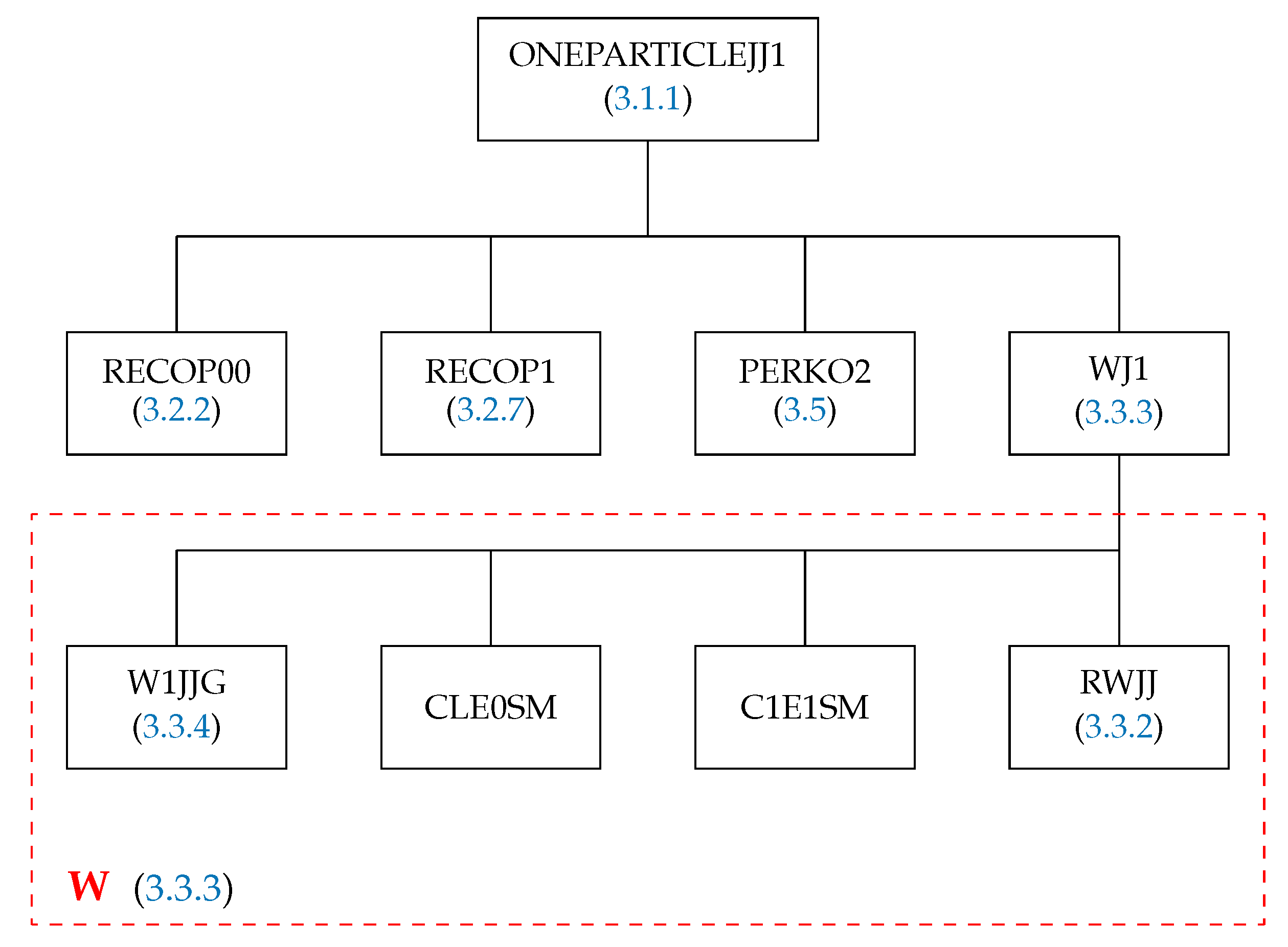
3.1.1. The Subroutine ONEPARTICLEJJ1

The purpose of the subroutine ONEPARTICLEJJ1 is to calculate the spin–angular coefficients of the diagonal matrix elements for the one-particle operator in the basis of configuration state functions (21). Its structure is presented in Figure 1. The subroutines RECOP00 and RECOP1 first of all check the selection rules for the recoupling coefficient. If it is nonzero, then the routine RECOP1 computes it (see Section 3.2.7 for more detail), but before it, the routine WJ computes matrix element (91) (see the red frame W in Figure 1, and a detailed description of it is in Section 3.3.3). The subroutine PERKO2 is the interface between GRASP-2018 [22] and the SQ routines group.
The subroutine has the following arguments:
  • NS is a number of peel subshells from the module m_C.
  • KA is a rank k of the operator (see (21)).
  • JJA and JJB are the numbers of configuration state functions for the matrix element to be evaluated.
  • JA is the index in the array JLIST of the orbital on which the creation operator acts.
  • JB is the index in the array JLIST of the orbital on which the annihilation operator acts.
  • COEFF is the value of the spin–angular part of the matrix element.

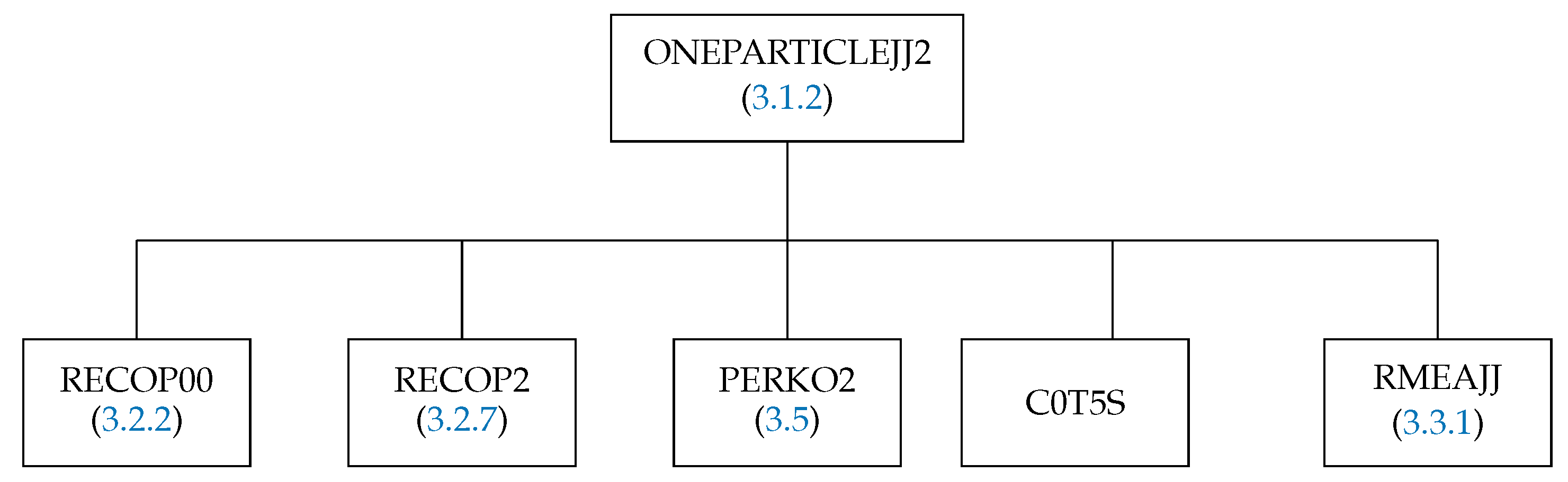
3.1.2. The Subroutine ONEPARTICLEJJ2

The purpose of the subroutine ONEPARTICLEJJ2 is to calculate the spin–angular coefficients of the off-diagonal matrix elements for the one-particle operator on the basis of configuration state functions (21). Its structure is presented in Figure 2. The subroutines RECOP00 and RECOP2 first of all check the selection rules for the recoupling coefficient. If it is nonzero, then the routine RECOP2 computes it (see Section 3.2.8 for more details), but before it, the routine C0T5S generates a Clebsch–Gordan coefficient depending on the occupation number of the subshell, and the routine RMEAJJ computes the reduced matrix element (89) (see Section 3.3.1). The subroutine PERKO2 is the interface between GRASP-2018 [22] and the SQ routines group.
The subroutine has the following arguments:
  • NS is a number of peel subshells from the module m_C.
  • KA is a rank k of the operator (see (21)).
  • JA is the index in the array JLIST of the orbital on which the creation operator acts.
  • JB is the index in the array JLIST of the orbital on which the annihilation operator acts.
  • COEFF is the value of the spin–angular part of the matrix element.

3.1.3. The Subroutines ONESCALAR1 and ONESCALAR2

The subroutines ONESCALAR1 and ONESCALAR2 have a similar structure as ONEPARTICLEJJ1 and ONEPARTICLEJJ2, respectively. They calculate the spin–angular coefficients of the matrix elements for the one-particle scalar operator in the basis of configuration state functions (8).

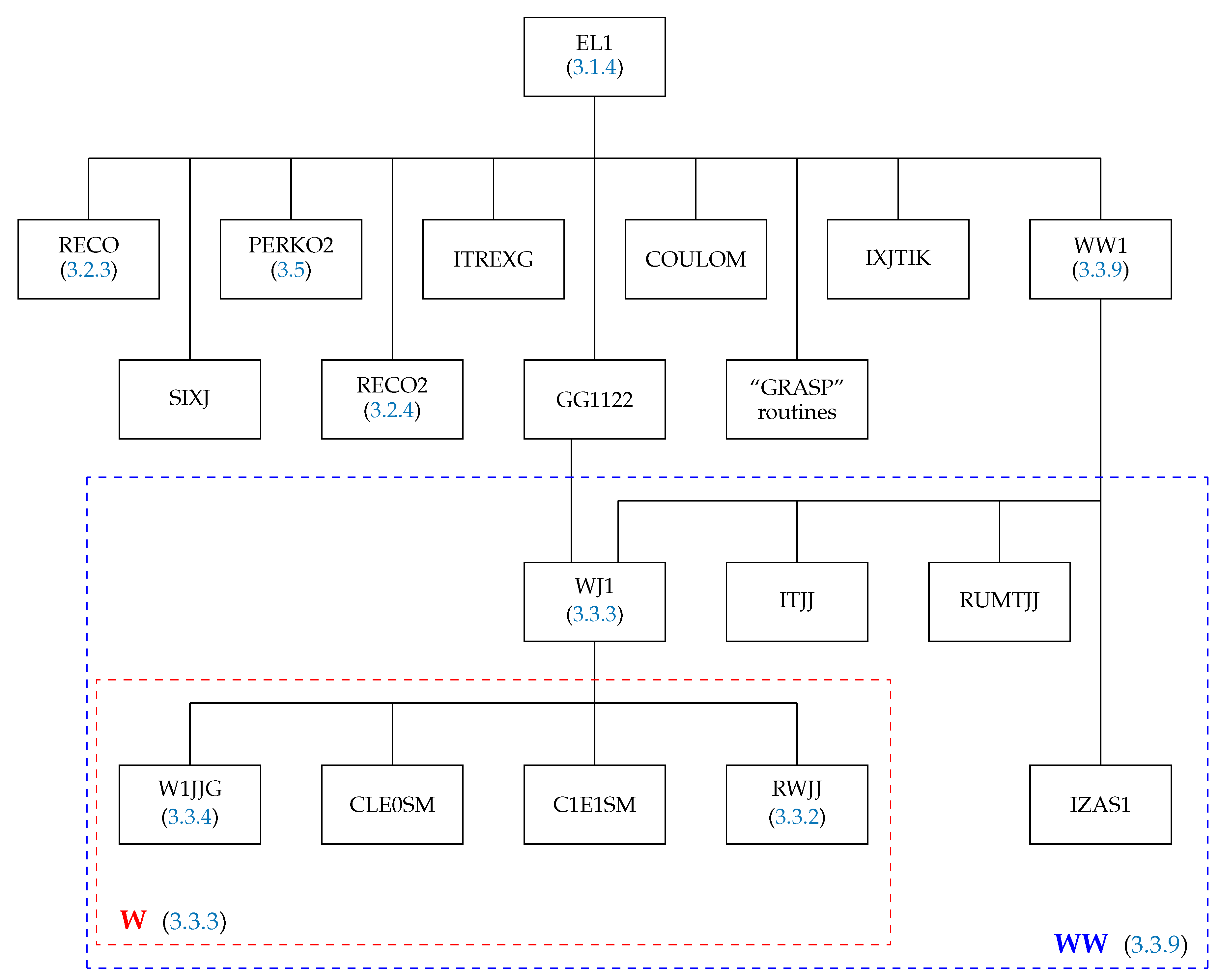
3.1.4. The Subroutine EL1

The purpose of the subroutine EL1 is to calculate the spin–angular coefficients of the diagonal matrix elements for the two-particle operator on the basis of configuration state functions (24). Its structure is presented in Figure 3. The subroutines RECO and RECO2 first of all check the selection rules for the recoupling coefficient. If it is nonzero, then the routine RECO2 computes it (see Section 3.2.4 for more details). The subroutine PERKO2 is the interface between GRASP-2018 [22] and the SQ routines group. The subroutines ITREXG and IXJTIK organize the calculation. The subroutine SIXJ calculates 6 j -coefficient. The subroutines SPEAK and TALK prepare the output of spin–angular coefficients for Coulomb and Breit interactions, respectively.
The spin-angular coefficients are actually computed by the subroutines WW1 and WJ1 from the routine GG1122. The first (see Figure 3 frame WW in blue frame) deals with cases such as
a ( j 1 ) ( n 1 l 1 ) a ( j 1 ) ( n 1 l 1 ) a ˜ ( j 1 ) ( n 1 l 1 ) a ˜ ( j 1 ) ( n 1 l 1 ) .
in which all the operators act on the same subshell. When there are two interacting subshells, the subroutine GG1122 organizes the calculation, which is actually performed by WJ1. For the direct case, the operator combinations are of the type
a ( j 1 ) ( n 1 l 1 ) a ( j 2 ) ( n 2 l 2 ) a ˜ ( j 1 ) ( n 1 l 1 ) a ˜ ( j 2 ) ( n 2 l 2 ) ,
a ( j 2 ) ( n 2 l 2 ) a ( j 1 ) ( n 1 l 1 ) a ˜ ( j 2 ) ( n 2 l 2 ) a ˜ ( j 1 ) ( n 1 l 1 ) ;
and for the exchange case, they are
a ( j 1 ) ( n 1 l 1 ) a ( j 2 ) ( n 2 l 2 ) a ˜ ( j 2 ) ( n 2 l 2 ) a ˜ ( j 1 ) ( n 1 l 1 )
a ( j 2 ) ( n 2 l 2 ) a ( j 1 ) ( n 1 l 1 ) a ˜ ( j 1 ) ( n 1 l 1 ) a ˜ ( j 2 ) ( n 2 l 2 ) .
WJ1 calls the subroutines in the red box W (in red frame) in Figure 3; a detailed description appears in Section 3.3.3.
The subroutine EL1 has the following arguments:
  • JJA and JJB are the numbers of configuration state functions for the matrix element to be evaluated.
  • JA and JB locate the position of the two interacting orbitals in the array JLIST [22] from the module m_C of GRASP-2018 [22] library Libmod. These parameters are used for the combinations (43)–(47).
  • IIRE must be set equal to 0 when the matrix element is diagonal , 1 when the matrix element is off-diagonal with respect to configuration state functions.
  • ICOLBREI determines the calculation of spin–angular coefficients 1 Coulomb interaction , 2 Breit interaction .

3.1.5. The Subroutine EL2

This calculates the spin-angular coefficients of the off-diagonal matrix elements of the two-particle operator (24) in the case when the bra and ket configurations have a pair of interacting shells whose occupation numbers differ by two
a ( j 1 ) ( n 1 l 1 ) a ( j 1 ) ( n 1 l 1 ) a ˜ ( j 2 ) ( n 2 l 2 ) a ˜ ( j 2 ) ( n 2 l 2 ) .
The structure of this subroutine is the same as that of EL1, omitting the subroutine WW1.
The subroutine has the following arguments:
  • JJA and JJB are the numbers of configuration state functions for the matrix element to be evaluated.
  • JA is the index in the array JLIST of the orbital on which the two creation operators act.
  • JB is the index in the array JLIST of the orbital on which the two annihilation operators act.
  • ICOLBREI determines the calculation of spin–angular coefficients 1 Coulomb interaction , 2 Breit interaction .

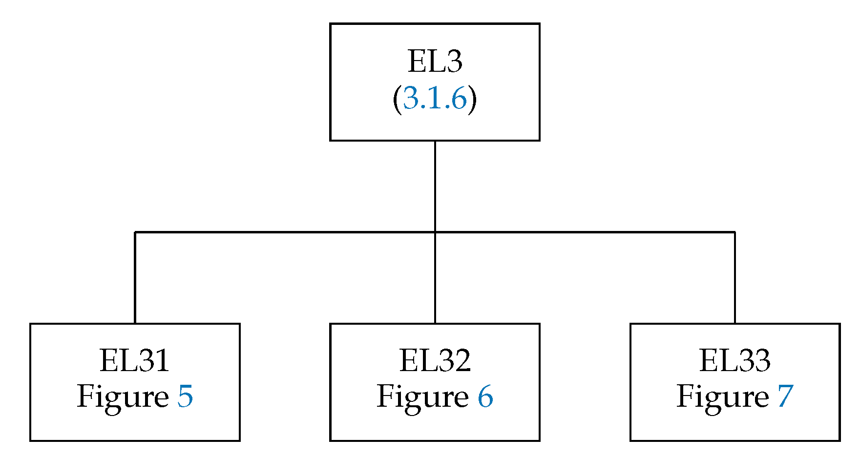
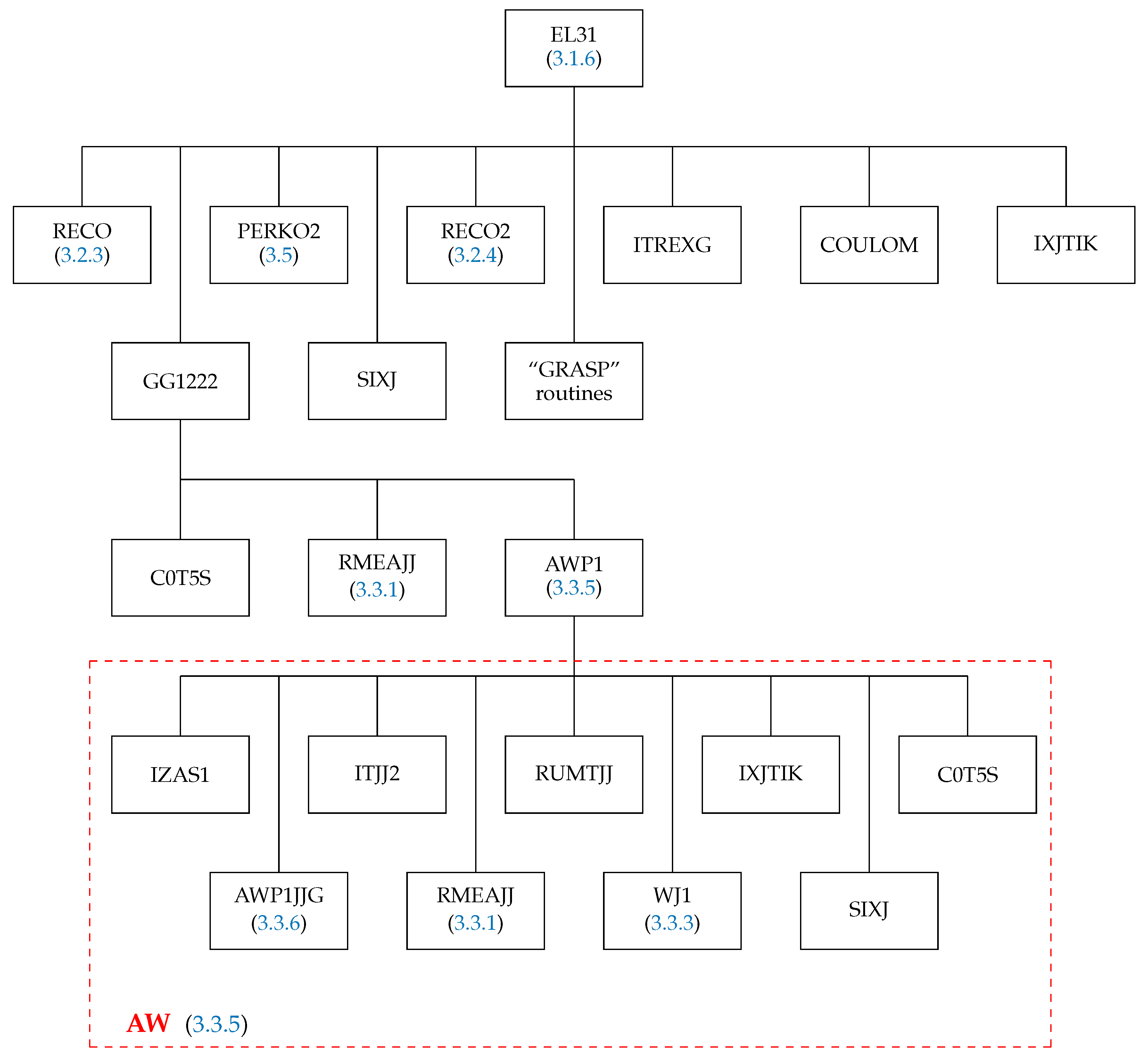
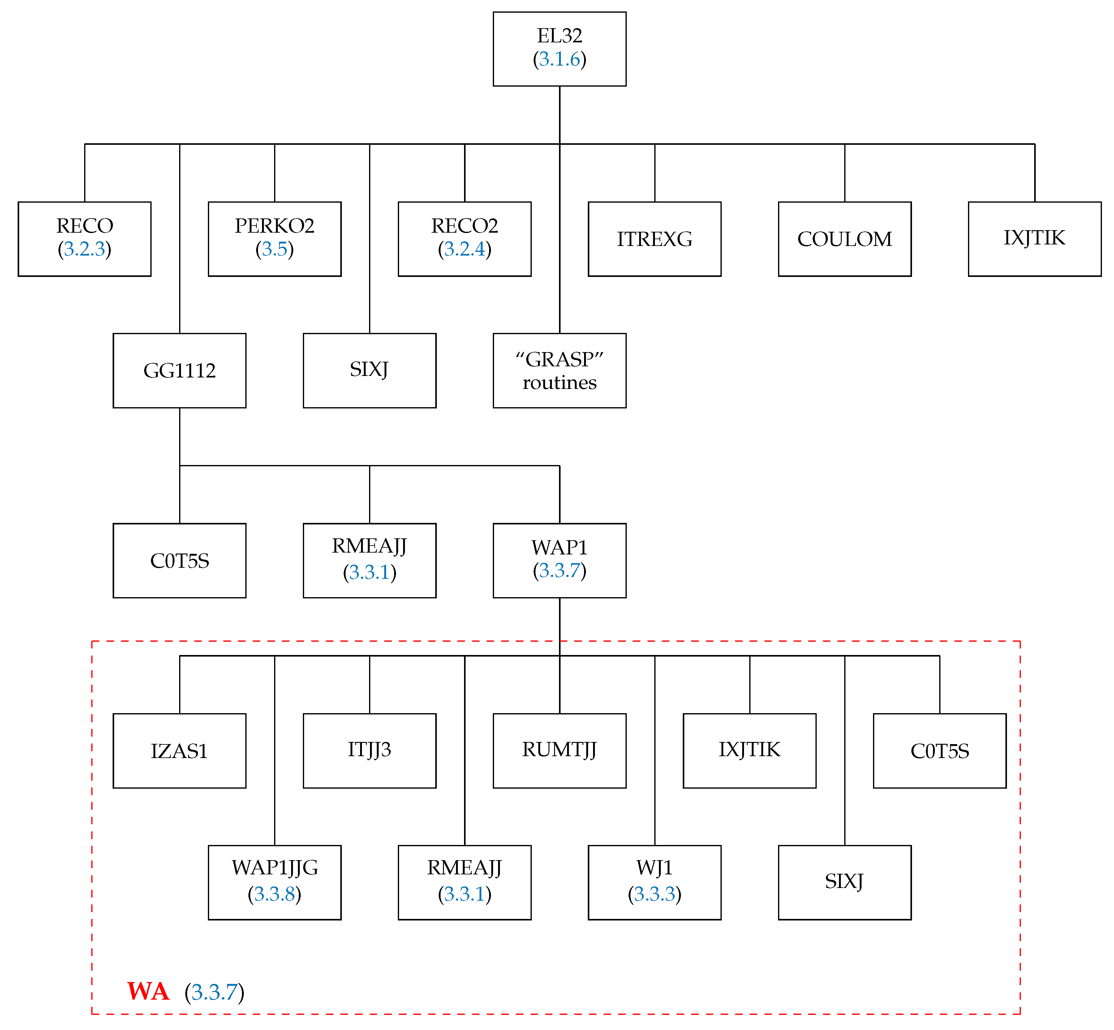
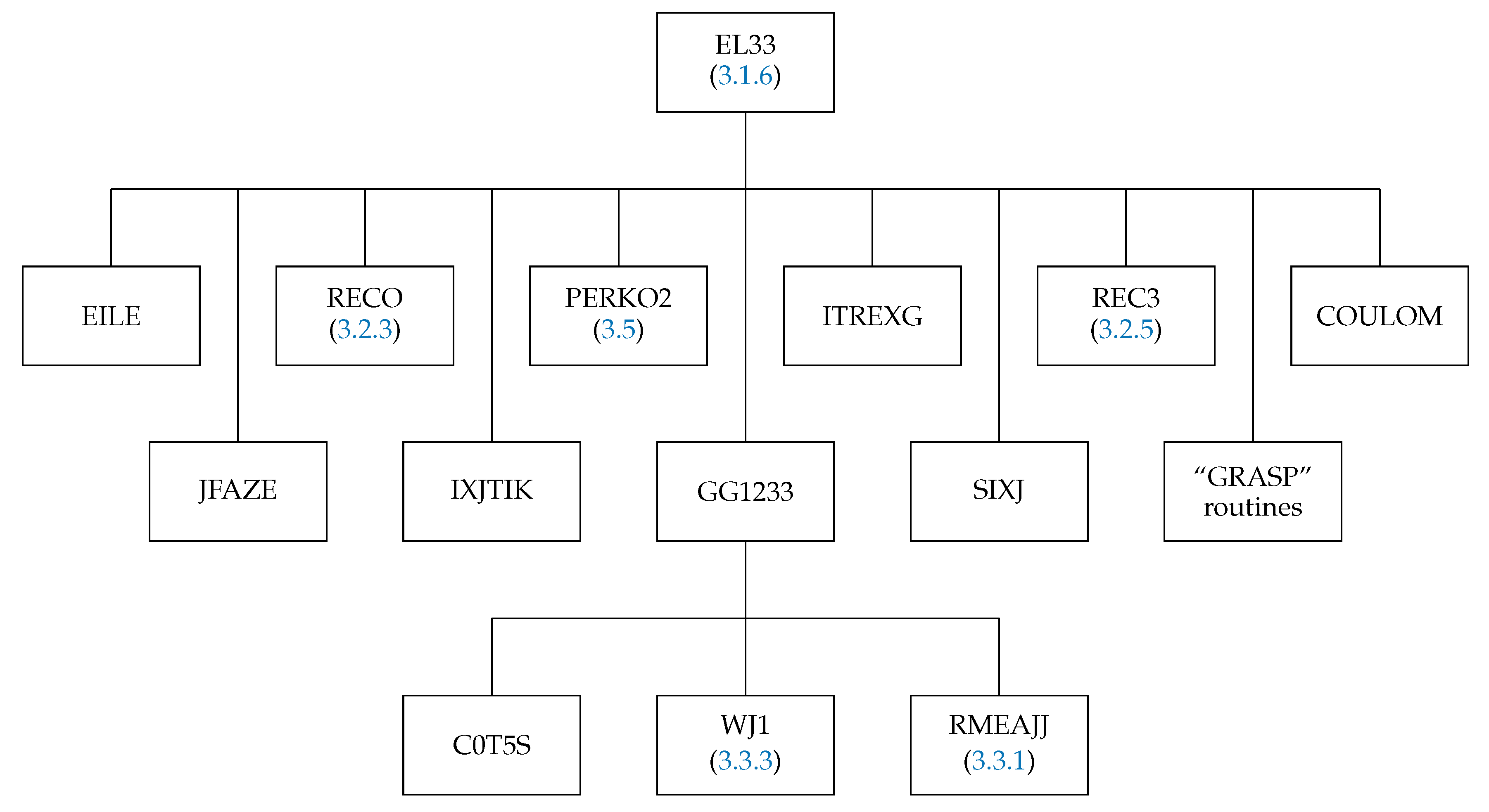
3.1.6. The Subroutine EL3

EL3 calculates the spin–angular coefficients of the off-diagonal matrix elements of the two-particle operator (24). The subshell occupation numbers of the bra configuration differ from those of the ket configuration by at most one. There are two interacting subshells on each side. The structure of this subroutine is presented in Figure 4.
The subroutine has a similar list of arguments as the routine EL2, but instead of the two arguments JA and JB it has four arguments, JA, JB, JC, and JD, which point to the interacting subshells of the matrix element of interest in the JLIST array.
The subroutine EL31 (Figure 5) determines the spin–angular coefficients for the operators
a ( j 2 ) ( n 2 l 2 ) a ( j 1 ) ( n 1 l 1 ) a ˜ ( j 1 ) ( n 1 l 1 ) a ˜ ( j 1 ) ( n 1 l 1 )
and
a ( j 1 ) ( n 1 l 1 ) a ( j 2 ) ( n 2 l 2 ) a ˜ ( j 1 ) ( n 1 l 1 ) a ˜ ( j 1 ) ( n 1 l 1 ) .
The structure of EL31 is very similar to that of EL1. The recoupling coefficient is the same as in (44)–(47), and the only additional subroutines are the C0T5S, which generates a Clebsch–Gordan coefficient depending on the occupation number of the second subshell, and the RMEAJJ from the routine GG1222, which provides the reduced matrix element of the a ( q j ) tensor operator. The subroutine AWP1 handles the more difficult calculation for the spin–angular part of the first shell. The structure of this subroutine is defined by the AW box (in red frame) in Figure 5; more details are given in Section 3.3.5.
The subroutine EL32 (Figure 6), which has a similar structure to EL31, calculates the spin–angular coefficients of the matrix elements for the combinations
a ( j 2 ) ( n 2 l 2 ) a ( j 2 ) ( n 2 l 2 ) a ˜ ( j 2 ) ( n 2 l 2 ) a ˜ ( j 1 ) ( n 1 l 1 )
and
a ( j 2 ) ( n 2 l 2 ) a ( j 2 ) ( n 2 l 2 ) a ˜ ( j 1 ) ( n 1 l 1 ) a ˜ ( j 2 ) ( n 2 l 2 ) .
The organization of EL32 is shown in Figure 6. The subroutine WAP1 organizes the more complicated calculation for the second subshell in this case. The structure of this subroutine is defined by the WA box (in red frame) in Figure 6; more details are given in Section 3.3.7.
The subroutine EL33 (Figure 7) calculates the spin–angular coefficients of the matrix elements for the three subshell cases
a ( j 2 ) ( n 2 l 2 ) a ( j 3 ) ( n 3 l 3 ) a ˜ ( j 1 ) ( n 1 l 1 ) a ˜ ( j 3 ) ( n 3 l 3 )
a ( j 3 ) ( n 3 l 3 ) a ( j 2 ) ( n 2 l 2 ) a ˜ ( j 3 ) ( n 3 l 3 ) a ˜ ( j 1 ) ( n 1 l 1 )
and
a ( j 3 ) ( n 3 l 3 ) a ( j 2 ) ( n 2 l 2 ) a ˜ ( j 1 ) ( n 1 l 1 ) a ˜ ( j 3 ) ( n 3 l 3 )
a ( j 2 ) ( n 2 l 2 ) a ( j 3 ) ( n 3 l 3 ) a ˜ ( j 3 ) ( n 3 l 3 ) a ˜ ( j 1 ) ( n 1 l 1 ) .
The routine RECO3 calculates the recoupling coefficient; more details are given in Section 3.2.5. The subroutine JFAZE determines the phase factor arising from operator permutations. The routine EILE reorders the subshells JA, JB, JC and places the ordered pointers in JAA, JBB, and JCC. The routine GG1233 organizes the calculation of the spin–angular coefficients. C0T5S determines two Clebsch–Gordan coefficients: one dependent on the occupation of the first subshell, the other on the occupation of the second subshell. RMEAJJ provides two reduced matrix elements of the a ( q j ) tensor operator, and WJ1 determines the spin–angular factors for the third shell (see Section 3.3.3).

3.1.7. The Subroutine EL4

The subroutine EL4 organizes the calculation of the spin–angular coefficients of off-diagonal matrix elements of the two-particle operator (24) involving three interacting subshells. The operator combinations are
a ( j 3 ) ( n 3 l 3 ) a ( j 3 ) ( n 3 l 3 ) a ˜ ( j 1 ) ( n 1 l 1 ) a ˜ ( j 2 ) ( n 2 l 2 ) ;
a ( j 3 ) ( n 3 l 3 ) a ( j 3 ) ( n 3 l 3 ) a ˜ ( j 2 ) ( n 2 l 2 ) a ˜ ( j 1 ) ( n 1 l 1 )
and
a ( j 1 ) ( n 1 l 1 ) a ( j 2 ) ( n 2 l 2 ) a ˜ ( j 3 ) ( n 3 l 3 ) a ˜ ( j 3 ) ( n 3 l 3 ) ;
a ( j 2 ) ( n 2 l 2 ) a ( j 1 ) ( n 1 l 1 ) a ˜ ( j 3 ) ( n 3 l 3 ) a ˜ ( j 3 ) ( n 3 l 3 ) .
It uses the subroutine EL41, which has the same structure as EL33 (Figure 7).
The subroutine EL4 has the arguments JJA and JJB, which define the numbers of configuration state functions for which the matrix element is to be evaluated, four arguments JA, JB, JC, and JD, which locate the interacting subshells in the array JLIST, and the argument ICOLBREI, which determines the calculation of spin–angular coefficients.

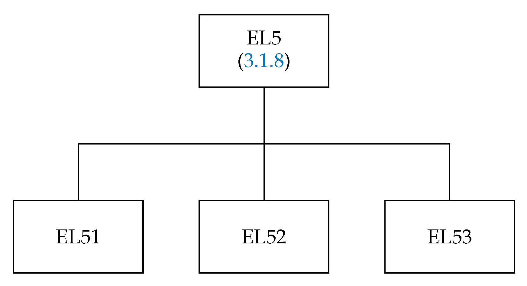
3.1.8. The Subroutine EL5

The EL5 calculates spin–angular coefficients of the off-diagonal matrix elements of the two-particle operator (24) when there are four interacting subshells. The structure of this routine is presented in Figure 8.
The subroutine EL5 has the arguments JJA and JJB, which define the numbers of configuration state functions for which the matrix element is to be evaluated, four arguments JA, JB, JC, and JD, which locate the interacting subshells in the array JLIST, and the argument ICOLBREI, which determines calculation of spin–angular coefficients.
The subroutine EL51 (Figure 9) is used for the operator combinations
a ( j 1 ) ( n 1 l 1 ) a ( j 2 ) ( n 2 l 2 ) a ˜ ( j 3 ) ( n 3 l 3 ) a ˜ ( j 4 ) ( n 4 l 4 ) ,
a ( j 2 ) ( n 2 l 2 ) a ( j 1 ) ( n 1 l 1 ) a ˜ ( j 4 ) ( n 4 l 4 ) a ˜ ( j 3 ) ( n 3 l 3 ) ;
a ( j 1 ) ( n 1 l 1 ) a ( j 2 ) ( n 2 l 2 ) a ˜ ( j 4 ) ( n 4 l 4 ) a ˜ ( j 3 ) ( n 3 l 3 ) ,
a ( j 2 ) ( n 2 l 2 ) a ( j 1 ) ( n 1 l 1 ) a ˜ ( j 3 ) ( n 3 l 3 ) a ˜ ( j 4 ) ( n 4 l 4 )
and
a ( j 3 ) ( n 3 l 3 ) a ( j 4 ) ( n 4 l 4 ) a ˜ ( j 1 ) ( n 1 l 1 ) a ˜ ( j 2 ) ( n 2 l 2 ) ,
a ( j 4 ) ( n 4 l 4 ) a ( j 3 ) ( n 3 l 3 ) a ˜ ( j 2 ) ( n 2 l 2 ) a ˜ ( j 1 ) ( n 1 l 1 ) ;
a ( j 3 ) ( n 3 l 3 ) a ( j 4 ) ( n 4 l 4 ) a ˜ ( j 2 ) ( n 2 l 2 ) a ˜ ( j 1 ) ( n 1 l 1 ) ,
a ( j 4 ) ( n 4 l 4 ) a ( j 3 ) ( n 3 l 3 ) a ˜ ( j 1 ) ( n 1 l 1 ) a ˜ ( j 2 ) ( n 2 l 2 ) .
The routines RECO and RECO4 generate the recoupling coefficient whenever it is nonzero (see Section 3.2.3 and Section 3.2.6). The GG1234 calculates the spin–angular coefficients for the cases (61)–(64) when the argument IREZ = 1 and the others (65)–(68) when IREZ = 2.
The subroutine EL52 handles the operator combinations
a ( j 1 ) ( n 1 l 1 ) a ( j 3 ) ( n 3 l 3 ) a ˜ ( j 2 ) ( n 2 l 2 ) a ˜ ( j 4 ) ( n 4 l 4 ) ,
a ( j 3 ) ( n 3 l 3 ) a ( j 1 ) ( n 1 l 1 ) a ˜ ( j 4 ) ( n 4 l 4 ) a ˜ ( j 2 ) ( n 2 l 2 ) ;
a ( j 1 ) ( n 1 l 1 ) a ( j 3 ) ( n 3 l 3 ) a ˜ ( j 4 ) ( n 4 l 4 ) a ˜ ( j 2 ) ( n 2 l 2 ) ,
a ( j 3 ) ( n 3 l 3 ) a ( j 1 ) ( n 1 l 1 ) a ˜ ( j 2 ) ( n 2 l 2 ) a ˜ ( j 4 ) ( n 4 l 4 )
and
a ( j 2 ) ( n 2 l 2 ) a ( j 4 ) ( n 4 l 4 ) a ˜ ( j 1 ) ( n 1 l 1 ) a ˜ ( j 3 ) ( n 3 l 3 ) ,
a ( j 4 ) ( n 4 l 4 ) a ( j 2 ) ( n 2 l 2 ) a ˜ ( j 3 ) ( n 3 l 3 ) a ˜ ( j 1 ) ( n 1 l 1 ) ;
a ( j 2 ) ( n 2 l 2 ) a ( j 4 ) ( n 4 l 4 ) a ˜ ( j 3 ) ( n 3 l 3 ) a ˜ ( j 1 ) ( n 1 l 1 ) ,
a ( j 4 ) ( n 4 l 4 ) a ( j 2 ) ( n 2 l 2 ) a ˜ ( j 1 ) ( n 1 l 1 ) a ˜ ( j 3 ) ( n 3 l 3 ) .
The structure of this routine is the same as that of EL51. It calculates the cases (69)–(72) when the argument IREZ = 1 and the others (73)–(76) when IREZ = 2.
Finally, EL53, which also has the same structure as EL51, treats the combinations
a ( j 1 ) ( n 1 l 1 ) a ( j 4 ) ( n 4 l 4 ) a ˜ ( j 2 ) ( n 2 l 2 ) a ˜ ( j 3 ) ( n 3 l 3 ) ,
a ( j 4 ) ( n 4 l 4 ) a ( j 1 ) ( n 1 l 1 ) a ˜ ( j 3 ) ( n 3 l 3 ) a ˜ ( j 2 ) ( n 2 l 2 ) ;
a ( j 1 ) ( n 1 l 1 ) a ( j 4 ) ( n 4 l 4 ) a ˜ ( j 3 ) ( n 3 l 3 ) a ˜ ( j 2 ) ( n 2 l 2 ) ,
a ( j 4 ) ( n 4 l 4 ) a ( j 1 ) ( n 1 l 1 ) a ˜ ( j 2 ) ( n 2 l 2 ) a ˜ ( j 3 ) ( n 3 l 3 )
and
a ( j 2 ) ( n 2 l 2 ) a ( j 3 ) ( n 3 l 3 ) a ˜ ( j 1 ) ( n 1 l 1 ) a ˜ ( j 4 ) ( n 4 l 4 ) ,
a ( j 3 ) ( n 3 l 3 ) a ( j 2 ) ( n 2 l 2 ) a ˜ ( j 4 ) ( n 4 l 4 ) a ˜ ( j 1 ) ( n 1 l 1 ) ;
a ( j 2 ) ( n 2 l 2 ) a ( j 3 ) ( n 3 l 3 ) a ˜ ( j 4 ) ( n 4 l 4 ) a ˜ ( j 1 ) ( n 1 l 1 ) ,
a ( j 3 ) ( n 3 l 3 ) a ( j 2 ) ( n 2 l 2 ) a ˜ ( j 1 ) ( n 1 l 1 ) a ˜ ( j 4 ) ( n 4 l 4 ) .
It handles the cases (77)–(80) when IREZ = 1 and the others (81)–(84) when IREZ = 2.

3.2. The REC Routines Group

This contains the following subroutines RECOONESCALAR, RECOP00, RECO, RECO2, REC3, RECO4, RECOP1, and RECOP2, all of which are concerned with the calculation of recoupling coefficients of one- or two- particle operators. The first checks that all of the second group of angular momentum selection rules coming from the recoupling coefficients R j i , j j , Λ b r a , a n d Λ k e t or R j i , j j , j i , j j , Λ b r a , Λ k e t , a n d Γ (see Table 1, Table 2 and Table 3) are satisfied and, if so, computes the recoupling coefficients for one, two, three or four subshells, respectively. The arrays and variables from the module m_C of Grasp2018 [22] library Libmod must be defined before calling REC.

3.2.1. The Subroutine RECOONESCALAR

This routine checks the first part of the second group of angular momentum selection rules coming from the recoupling coefficients R j i , j j , Λ b r a , Λ k e t , and Γ (see Table 1) for the one-particle scalar operator.
The subroutine RECOONESCALAR has the following arguments:
  • NS is the number of peel subshells from the module m_C for the diagonal case and NS = -1 for the off-diagonal matrix element.
  • JA1 identifies the first subshell, on which the creation operator a ( j ) or annihilation tensor a ˜ ( j ) acts in the array JLIST.
  • JA2 identifies the second subshell, on which the creation operator a ( j ) or annihilation tensor a ˜ ( j ) acts in the array JLIST. The subshells must be numbered so that the arguments JA1 and JA2 are in an increasing order.
  • KA is the parameter which determines the number of subshells coupled by the interaction, taking the values K A = 0 if one subshell , K A = 1 if two subshells .
  • The subroutine returns the value of IAT, which is 0 if the selection rules are not satisfied and the recoupling coefficient is zero , 1 if the recoupling coefficient is to be calculated .

3.2.2. The Subroutine RECOP00

This routine checks the first part of the second group of angular momentum selection rules coming from the recoupling coefficients R j i , j j , Λ b r a , Λ k e t , Γ (see Table 2) for the one-particle nonscalar operator.
The subroutine RECOP00 has the following arguments:
  • NS is the number of peel subshells from the module m_C for the diagonal case and NS = -1 for the off-diagonal matrix element.
  • JA1 identifies the first subshell, on which the creation operator a ( j ) or annihilation tensor a ˜ ( j ) acts in the array JLIST.
  • JA2 identifies the second subshell, on which the creation operator a ( j ) or annihilation tensor a ˜ ( j ) acts in the array JLIST. The subshells must be numbered so that the arguments JA1 and JA2 are in an increasing order.
  • KA is the rank k of the operator.
  • The subroutine returns the value of IAT, which is 0 if the selection rules are not satisfied and the recoupling coefficient is zero , 1 if the recoupling coefficient is to be calculated .

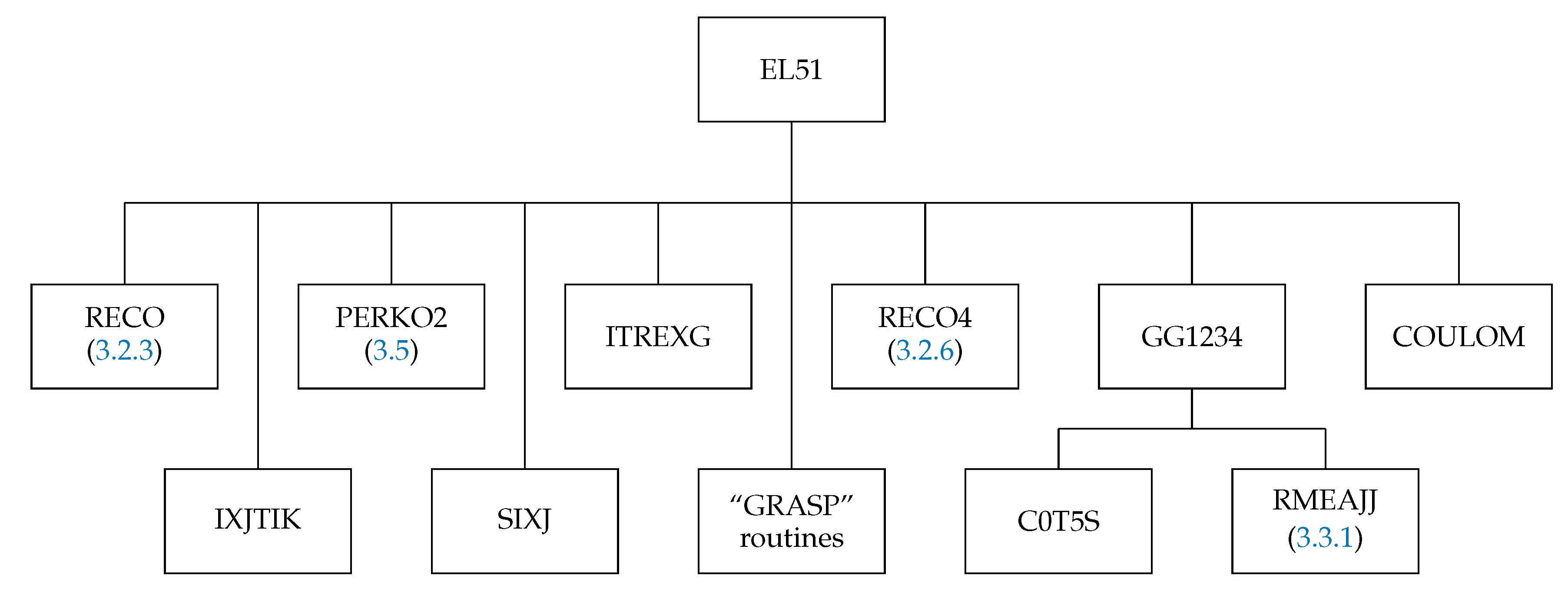
3.2.3. The Subroutine RECO

This routine checks the first part of the second group of angular momentum selection rules coming from the recoupling coefficients R j i , j j , j i , j j , Λ b r a , Λ k e t , and Γ (see Table 3) for the two-particle operator. It has the arguments JA1, JA2, JA3, and JA4, which point to the relevant orbitals in the array JLIST [22] from the module m_C of GRASP-2018 [22] library Libmod. The subshells must be numbered so that the arguments are in an increasing order.
KA is the parameter which determines the number of subshells coupled by the interaction, taking the values
  • KA = 0, in one subshell or in two subshells when the intermediate rank of the operator is equal to zero.
  • KA = 1, in two subshells when the intermediate rank of the operator is nonzero.
  • KA = 2, three subshells.
  • KA = 3, four subshells.
The subroutine returns the number IAT, where
  • IAT = 0 if the recoupling coefficient is zero.
  • IAT = 1 otherwise.

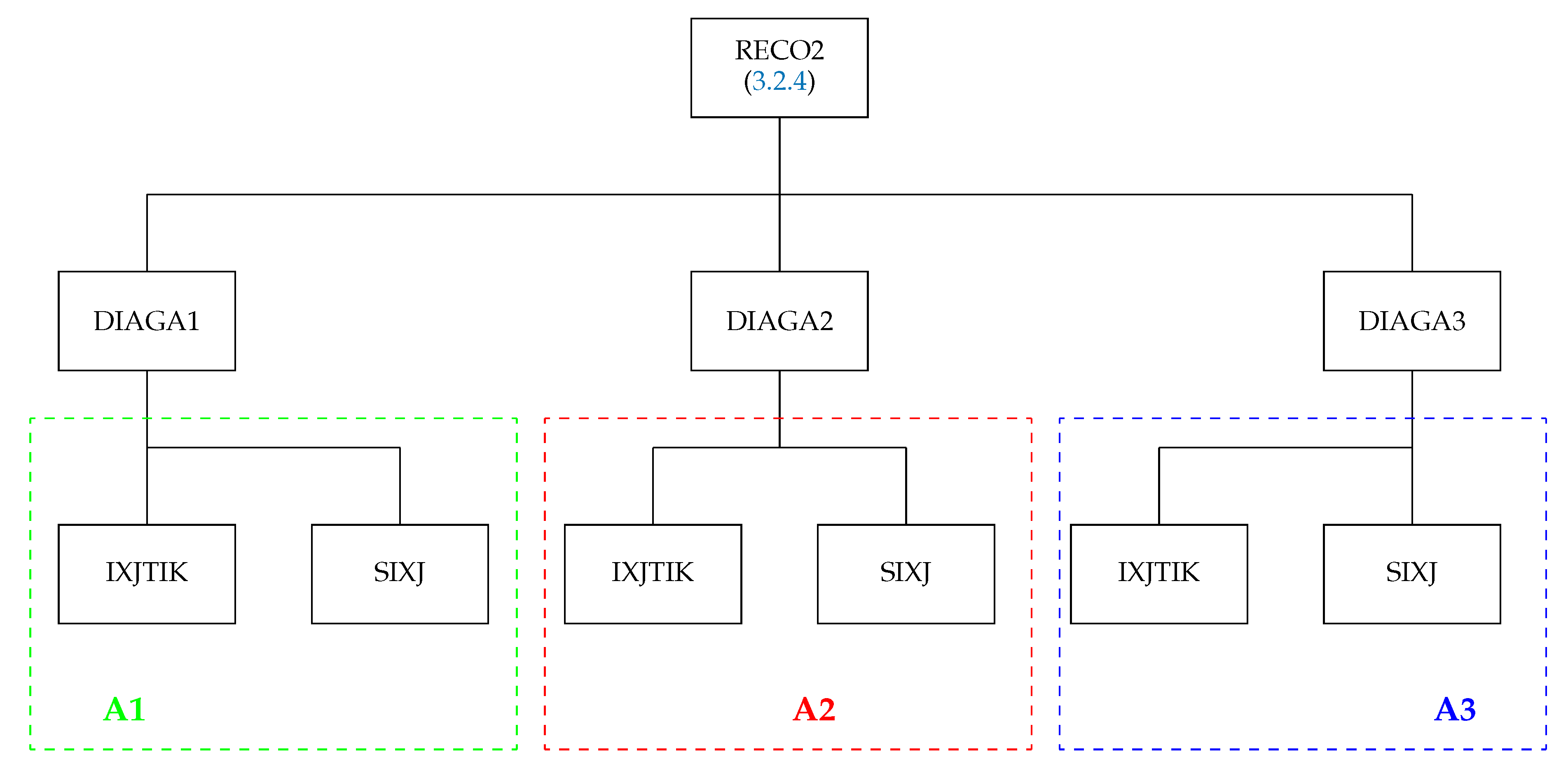
3.2.4. The Subroutine RECO2

This subroutine checks the second part of the second group of angular momentum selection rules coming from R j i , j j , j i , j j , Λ b r a , Λ k e t , and Γ (see Table 3)) or calculates the recoupling coefficients for the one- and the two-particle scalar operators acting in two different subshells, the tensorial structure of which can be represented as
A ( k ) ( n 1 j 1 ) × B ( k ) ( n 2 j 2 ) ( 0 ) .
where A ( k ) and B ( k ) are simple or composite tensor operators of rank k. A ( k ) acts only on the first active shell and B ( k ) on the second active shell in the order in which they are coupled in the configuration.
The structure of the routine is presented in Figure 10. In most cases, the recoupling coefficients factorize in three parts which are generated by the subroutines DIAGA1, DIAGA2, and DIAGA3. When the argument IRE = 0, all triads of the recoupling coefficient are checked using the routine IXJTIK and perform the actual calculation when IRE = 1. The necessary 6 j -coefficients are generated using SIXJ.
The subroutine RECO2 has the following arguments:
  • JA1 identifies the first subshell on which the operator A ( k ) acts in the array JLIST.
  • JA2 identifies the second subshell on which the operator B ( k ) acts in the array JLIST.
  • KA is the intermediate rank k.
  • IRE takes the input value 0 if only the coupling triads are to be checked 1 if the recoupling coefficient is to be calculated .
  • When IRE = 0, the subroutine returns the value of IAT, which is 0 if the selection rules are not satisfied and the recoupling coefficient is zero , 1 if the recoupling coefficient is to be calculated .
  • REC is the value of the recoupling coefficient computed when IRE = 1.

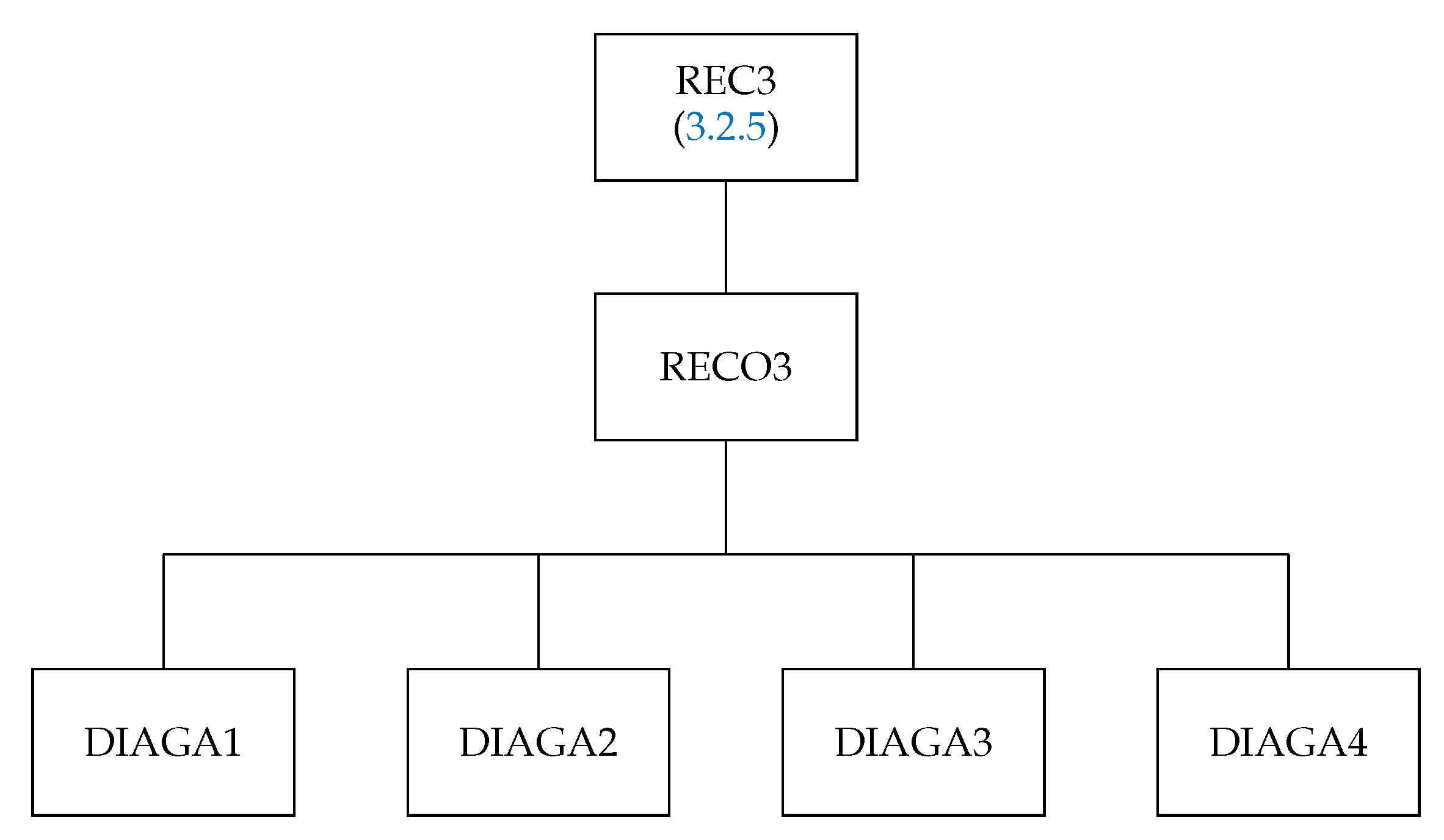
3.2.5. The Subroutine REC3

This subroutine checks the second part of the second group of angular momentum selection rules coming from R j i , j j , j i , j j , Λ b r a , Λ k e t , and Γ or calculates the recoupling coefficients for the two-particle scalar operator acting in three different subshells, the tensorial structure of which can be represented as
A ( k 1 ) ( n i j i ) × B ( k 2 ) ( n j j j ) ( k ) × C ( k ) ( n m j m ) ( 0 ) .
As in (85), A ( k 1 ) , B ( k 2 ) , and C ( k ) are simple or composite tensor operators which act on subshells i, j, and m, respectively.
The structure of the routine is presented in Figure 11. The recoupling coefficients can be factorized into several simple parts, which are generated by the subroutines DIAGA1, DIAGA2, DIAGA3, and DIAGA4. REC3 checks all triads of the recoupling coefficient using IXJTIK if IRE = 0 and performs the calculation if IRE = 1.
The subroutine has the following arguments:
  • JA1, JA2, and JA3, which point to the orbitals i, j, and m in the array JLIST.
  • K1, K2, and KA, which are the ranks k 1 , k 2 , and k of the component tensor operators (86).
  • IRE takes the input value 0 if only the coupling triads are to be checked 1 if the recoupling coefficient is to be calculated .
  • When IRE = 0, the subroutine returns the value of IAT, which is 0 if the selection rules are not satisfied and the recoupling coefficient is zero , 1 if the recoupling coefficient is to be calculated .
  • REC is the value of the recoupling coefficient computed when IRE = 1.

3.2.6. The Subroutine RECO4

This subroutine checks the second part of the second group of angular momentum selection rules coming from R j i , j j , j i , j j , Λ b r a , Λ k e t , and Γ or calculates the recoupling coefficients for the two-particle scalar operator acting in four different subshells, the tensorial structure of which can be represented as
A ( k 1 ) ( n 1 j 1 ) × B ( k 2 ) ( n 2 j 2 ) ( k ) × C ( k 3 ) ( n 3 j 3 ) × D ( k 4 ) ( n 4 j 4 ) ( k ) ( 0 ) ,
where A ( k 1 ) , B ( k 2 ) , C ( k 3 ) , and D ( k 4 ) may be simple or composite tensor operators of the orders indicated, corresponding to the structure of (87). The subshells must be ordered so that A ( k 1 ) operates on the first and D ( k 4 ) on the last in order.
The structure of the subroutine RECO4 is the same as that of RECO3 (Figure 11).
The subroutine has the following arguments:
  • JA1, JA2, JA3, and JA4, which point to the orbitals 1, 2, 3, and 4 in the array JLIST.
  • K1, K2, K3, K4, and KA, which are the ranks k 1 , k 2 , k 3 , k 4 , and k of the component tensor operators (87).
  • IRE takes the input value 0 if only the coupling triads are to be checked 1 if the recoupling coefficient is to be calculated .
  • When IRE = 0, the subroutine returns the value of IAT, which is 0 if the selection rules are not satisfied and the recoupling coefficient is zero , 1 if the recoupling coefficient is to be calculated .
  • REC is the value of the recoupling coefficient computed when IRE = 1.

3.2.7. The Subroutine RECOP1

This subroutine checks the second part of the second group of angular momentum selection rules coming from R j i , j j , Λ b r a , and Λ k e t (see Table 2)) or calculates the recoupling coefficients for the one-particle nonscalar operator acting in one subshell.
The structure of the subroutine RECOP1 is similar to that of RECO2 (Figure 10), except that DIAGA5 is used instead of DIAGA2.
The subroutine RECOP1 has the following arguments:
  • NS is the number of peel subshells from the module m_C.
  • JA1 identifies the subshell on which the operator a 1 / 2 q j × a 1 / 2 q j k acts in the array JLIST.
  • KA is the intermediate rank k.
  • IRE takes the input value 0 if only the coupling triads are to be checked 1 if the recoupling coefficient is to be calculated .
  • When IRE = 0, the subroutine returns the value of IAT, which is 0 if the selection rules are not satisfied and the recoupling coefficient is zero , 1 if the recoupling coefficient is to be calculated .
  • RECC is the value of the recoupling coefficient computed when IRE = 1.

3.2.8. The Subroutine RECOP2

This subroutine checks the second part of the second group of angular momentum selection rules coming from R j i , j j , Λ b r a , and Λ k e t (see Table 2) or calculates the recoupling coefficients for the one-particle nonscalar operator acting in two different subshells, the tensorial structure of which can be represented as
A ( k 1 ) ( n 1 j 1 ) × B ( k 2 ) ( n 2 j 2 ) ( k ) .
where A ( k ) and B ( k ) are simply the creation operator a ( j ) or annihilation tensor a ˜ ( j ) . A ( k ) acts only on the first active subshell and B ( k ) on the second active subshell in the order in which they are coupled in the configuration.
The structure of the subroutine RECOP2 is similar to that of RECO3 (Figure 11), except that DIAGA5 is used instead of DIAGA2.
The subroutine has the following arguments:
  • NS is the number of peel subshells from the module m_C.
  • JA1 and JA2, which point to the orbitals 1 and 2 in the array JLIST.
  • K1, K2, and KA, which are the ranks k 1 , k 2 , and k of the component tensor operators (88).
  • IRE takes the input value 0 if only the coupling triads are to be checked 1 if the recoupling coefficient is to be calculated .
  • When IRE = 0, the subroutine returns the value of IAT, which is 0 if the selection rules are not satisfied and the recoupling coefficient is zero , 1 if the recoupling coefficient is to be calculated .
  • RECC is the value of the recoupling coefficient computed when IRE = 1.

3.3. The SQ Routines Group

The Section SQ (standard quantities) is a collection of utilities used by the routines groups METWO and REC. Most of them are independent and may be used in other programs. The routines check the third group of angular momentum selection rules (see Table 1, Table 2 and Table 3) by mainly calling the routines ITJJ, IXJTIK, C0T5S, C1E0SM, C1E1SM, and CLE0SM and, if so, calculates the matrix or reduced matrix elements of standard quantities.
Most of the subroutines use arrays from the module CONS_C of Grasp2018 [22] library Libmod. Single subshell data needed for calculation are stored in the two arrays I and B. The former consists of:
  • I(1), which is the state number of the subshell (see column  N o . in Table 4).
  • I(2), which is the principal quantum number n.
  • I(3), which is the quantum number j multiplied by two.
  • I(4), which is the number of electrons in the subshell.
  • I(5), which is the orbital quantum number l.
  • I(6), which is the subshell total angular momentum J multiplied by two.
  • I(7), which is the subshell total quasi-spin Q multiplied by two.
The array B contains:
  • B(1), which is the subshell quasi-spin Q.
  • B(2), which is the subshell total angular momentum J.
  • B(3), which is the subshell quasi-spin projection M Q .

3.3.1. The Subroutine RMEAJJ

This subroutine determines the value of the reduced matrix elements of operator (25)
j α Q J a ( q j ) j α Q J .
The subroutine uses the table of reduced matrix elements of the
a ( q j )
tensor operator for j = 1 / 2 9 / 2 , which are stored in memory.
The subroutine has the following arguments:
  • LL is the quantum number j multiplied by two.
  • IT is the state number of the bra function (see column  N o . in Table 4).
  • LQ is the quasi-spin Q for the bra function multiplied by two.
  • J is the total angular momentum J for the bra function multiplied by two.
  • ITS is the state number of the ket function.
  • LQS is the quasi-spin Q for the ket function multiplied by two.
  • J1S is the total angular momentum J for the ket function multiplied by two.
  • COEF is the value of the reduced matrix element (89) which is returned by the subroutine.

3.3.2. The Subroutine RWJJ

The subroutine determines the value of the reduced matrix element of operator (26)
j α Q J a ( q j ) × a ( q j ) ( k 1 k 2 ) j α Q J .
The subroutine uses the table of reduced matrix elements of the tensor operator
a ( q j ) × a ( q j ) ( k 1 k 2 )
stored in memory for j = 1 / 2 7 / 2 .
The subroutine has the following arguments:
  • J is the quantum number j multiplied by two.
  • J1 is the state number of the bra function.
  • J2 is the state number of the ket function.
  • K1 is the rank k 1 (see (90)).
  • K2 is the rank k 2 (see (90)).
  • COEF is the value of the reduced matrix element (90) which is returned by the subroutine.

3.3.3. The Subroutine WJ1

Before determining the value of the matrix element of operator (26)
( n ) j w α Q J a m q 1 ( q j ) × a m q 2 ( q j ) ( k ) n ) j w α Q J ,
this subroutine checks the main part of the third group of angular momentum selection rules coming from
T j i , j j , j i , j j , Λ b r a , Λ k e t , Ξ , Γ
for j = 1 / 2 37 / 2 (see Table 3).
The subroutines calls W1JJG for the calculation of the matrix element (91) in cases j = 9 / 2 37 / 2 . The subroutine finds the Clebsch–Gordan coefficient, which gives the dependence on the subshell occupation number in cases j = 1 / 2 7 / 2 . If the tensor product (91) consists of either two electron creation operators or two annihilation operators, then C1E1SM is called. Otherwise, C1E0SM is called. The subroutine RWJJ finds the reduced matrix elements of the operator a ( q j ) × a ( q j ) ( k 1 k 2 ) . The structure of the subroutine WJ1 is given in the red box labeled W in Figure 3.
The subroutine has the following arguments:
  • IK is the array I for the bra function.
  • BK is the array B for the bra function.
  • ID is the array I for the ket function.
  • BD is the array B for the ket function.
  • K2 is the rank k (see (91)).
  • QM1, QM2 are the quasi-spin projections in (91).
  • WJ is the value of the reduced matrix element (91) which is returned by the subroutine.

3.3.4. The Subroutine W1JJG

This subroutine determines the value of the matrix element (91) for j = 9 / 2 37 / 2 .
The subroutine has the following arguments:
  • K1 is the rank k (see (91)).
  • QM1 and QM2 are the quasi-spin projections in (91).
  • IK is the array I for the bra function.
  • BK is the array B for the bra function.
  • ID is the array I for the ket function.
  • BD is the array B for the ket function.
  • WW is the value of the reduced matrix element (91) which is returned by the subroutine.

3.3.5. The Subroutine AWP1

Before determining the value of the matrix elements element of operator (27)
( n ) j w α Q J a m q 1 ( q j ) × a m q 2 ( q j ) × a m q 3 ( q j ) ( k 1 ) ( k ) ( n ) j w α Q J ,
the subroutine checks the main part of the third group of angular momentum selection rules coming from
T j i , j j , j i , j j , Λ b r a , Λ k e t , Ξ , Γ
for j = 1 / 2 37 / 2 (see Table 3).
The subroutine calls AWP1JJG for the calculation of the matrix element (92) in cases j = 9 / 2 37 / 2 . The subroutine IZAS1 checks that the subshell has a state with the specified characteristics in cases j = 1 / 2 7 / 2 . The subroutine ITJJ2 finds the first and the last numbers of the state from the running intermediate sum over term numbers (see column  N o . in Table 4). The RUMT finds the subshell total angular momentum J and quasi-spin Q for each intermediate state. The subroutine IXJTIK checks all triads. The subroutine C0T5S finds the Clebsch–Gordan coefficient giving the dependence on the subshell occupation number, and the RMEAJJ finds the reduced matrix element of the a ( q j ) tensor operator (see in Section 3.3.1). The second part of the expression is calculated by the subroutine WJ1 (see in Section 3.3.3). The subroutine SIXJ finds the 6 j -coefficient. The structure of the subroutine AWP1 is presented as a red box AW in Figure 5.
The subroutine has the following arguments:
  • IK is the array I for the bra function.
  • BK is the array B for the bra function.
  • ID is the array I for the ket function.
  • BD is the array B for the ket function.
  • K1 is the rank k 1 (see (92)).
  • BK2 is the rank k (see (92)).
  • QM1, QM2, and QM3 are the quasi-spin projections in (92).
  • AW is the value of the reduced matrix element (92) which is returned by the subroutine.

3.3.6. The Subroutine AWP1JJG

The subroutine determines the value of the matrix elements (92) for j = 9 / 2 37 / 2 .
The subroutine has the following arguments:
  • K1 is the rank k 1 (see (92)).
  • BK2 is the rank k (see (92)).
  • QM1, QM2, and QM3 are the quasi-spin projections in (92).
  • IK is the array I for the bra function.
  • BK is the array B for the bra function.
  • ID is the array I for the ket function.
  • BD is the array B for the ket function.
  • AW is the value of the reduced matrix element (92) which is returned by the subroutine.

3.3.7. The Subroutine WAP1

Before determining the value of the matrix elements of operator (28)
( n ) j w α Q J a m q 1 ( q j ) × a m q 2 ( q j ) ( k 1 ) × a m q 3 ( q j ) ( k ) ( n ) j w α Q J ,
this subroutine checks the main part of the third group of angular momentum selection rules coming from
T j i , j j , j i , j j , Λ b r a , Λ k e t , Ξ , Γ
for j = 1 / 2 37 / 2 (see Table 3).
The structure of the subroutine WAP1 is the same as that of the AWP1, shown as a red box WA in Figure 6. The subroutine calls WAP1JJG for the calculation of the matrix element (93) in cases j = 9 / 2 37 / 2 . The WJ1 is used for the first part of the operator and C0T5S and RMEAJJ for the second part in cases j = 1 / 2 7 / 2 .
The subroutine has the following arguments:
  • IK is the array I for the bra function.
  • BK is the array B for the bra function.
  • ID is the array I for the ket function.
  • BD is the array B for the ket function.
  • K1 is the rank k 1 (see (93)).
  • BK2 is the rank k (see (93)).
  • QM1, QM2, and QM3 are the quasi-spin projections in (93).
  • WA is the value of the reduced matrix element (93) which is returned by the subroutine.

3.3.8. The Subroutine WAP1JJG

The subroutine determines the value of the matrix elements (93) for j = 9 / 2 37 / 2 .
The subroutine has the following arguments:
  • K1 is the rank k 1 (see (93)).
  • BK2 is the rank k (see (93)).
  • QM1, QM2, and QM3 are the quasi-spin projections in (93).
  • IK is the array I for the bra function.
  • BK is the array B for the bra function.
  • ID is the array I for the ket function.
  • BD is the array B for the ket function.
  • WA is the value of the reduced matrix element (93) which is returned by the subroutine.

3.3.9. The Subroutine WW1

Before determining the value of matrix elements of operator (29)
( n ) j w α Q J a m q 1 ( q j ) × a m q 2 ( q j ) ( k ) × a m q 3 ( q j ) × a m q 4 ( q j ) ( k ) ( 0 ) ( n ) j w α Q J ,
the subroutine checks the main part of the third group of angular momentum selection rules coming from
T j i , j j , j i , j j , Λ b r a , Λ k e t , Ξ , Γ
for j = 1 / 2 37 / 2 (see Table 3).
The subroutine WW1 uses the subroutines ITJJ, RUMT, and IZAS1 for calculation of this sort of matrix element. The subroutine WJ1 calculates the first and the second parts of the operator to be calculated. The structure of the subroutine WW1 is presented in Figure 3 (blue block WW).
The subroutine has the following arguments:
  • IK is the array I for the bra function.
  • BK is the array B for the bra function.
  • ID is the array I for the ket function.
  • BD is the array B for the ket function.
  • K2 is the rank k (see (94)).
  • QM1, QM2, QM3, and QM4 are the quasi-spin projections in (94).
  • WW is the value of the reduced matrix element (94) which is returned by the subroutine.

3.4. Description of the New Modules for Arrays Used in the Program Library

The principal new developed modules for arrays used in the program library are listed in the Table 5. They are located in the GRASP-2018 [22] library Libmod.

3.5. Interface between the Program Library and GRASP

Two subroutines, PERKO1 and PERKO2, serve as the interface between GRASP-2018 [22] and the present program library. The call of subroutine PERKO2 to subroutine PERKO1 depends on how many interacting subshells are used for evaluating the matrix element. The subroutine PERKO1 fills the arrays I and B (see Section 3.3)) from the arrays NQ1, NQ2, JJQ1, JJQ2, NP, and NAK of the modules m_C and orb_C located in GRASP-2018 [22] library Libmod.

3.6. Installation Features in the GRASP

This program library evaluates any matrix element of energy structure (Dirac–Coulomb–Breit Hamiltonian H D C B ) [5] and atomic property (hyperfine structure, transition parameters, and isotope shift) [23] operators of spin–angular coefficients with any number of open subshells. The library, depending on the complexity of the evaluated case, provides the spin–angular coefficients with different speed. If the case is simple (for example Dirac–Coulomb Hamiltonian H D C ) and does not have too many open shells or has features described in Section 2.4.4, then it is calculated at the highest speed. So, it is not necessary to use simple analytical expressions of spin–angular coefficients, such as discussed in Section 2.4.4, for applying this library in some program packages (for example, GRASP-2018 [22]). However, the GRASP-2018 [22] package has fragments of the program written in the 1980s [51]. So, the program rmcdhf operates in such a way that it reduces the usage of disk space. Therefore, this program has two routines, FCO and GCO, which calculate some simple spin–angular coefficients on the fly. The routine FCO of any version of the GRASP package [22,35,52,54,55] evaluates the spin–angular coefficients presented in (36), (37), and (40). The routine GCO of any version of the GRASP package [22,35,52,54,55] evaluates the spin–angular coefficient (41). The subroutine ONESCALAR (see the routine mcp in the Rangular program) provides the rest of the spin–angular coefficients, and the program rmcdhf reads them from the files mcp.*.

3.7. A Speed-Up in Calculations with the Present Program Library Integrated in GRASP Package

The program library is designed for large-scale atomic structure calculations, and its computational cost is less than that of the corresponding spin–angular modules of GRASP [52,54,55].
Here, we present timing studies using the Dirac–Coulomb Hamiltonian for the 3 s 2 3 p 6 1 S state of Ar I with the common closed shells 1 s 2 2 s 2 2 p 6 for different values of final orbital momentum J. The wave function expansions used were:
  • 3SD: Single and double excitations from 3 s 2 3 p 6 to the active set { 3 s , 3 p , 3 d } containing 14 configuration state functions (CSF) for J = 0 and 34 CSF (the maximum) for J = 2 .
  • 3SDT: Single, double, and triple excitations from 3 s 2 3 p 6 to the active set { 3 s , 3 p , 3 d } . The maximum number of CSF is 145 for J = 2 .
  • 4SD: Single and double excitations from 3 s 2 3 p 6 to the active set
    { 3 s , 3 p , 3 d , 4 s , 4 p , 4 d , 4 f } . The maximum number of CSF is 465 for J = 2 .
  • 4SDT: Single, double, and triple excitations from 3 s 2 3 p 6 to the active set
    { 3 s , 3 p , 3 d , 4 s , 4 p , 4 d , 4 f } .
  • 5SD; Single and double excitations from 3 s 2 3 p 6 to the active set
    { 3 s , 3 p , 3 d , 4 s , 4 p , 4 d , 4 f , 5 s , 5 p , 5 d , 5 f , 5 g } .
Let us first consider simple cases with a small number of CSFs (3SD, 3SDT, and 4SD with J = 0, 1, 2, 3, 4, 5, 6, 7, 8, 9). Although GRASP(New) [22,35] with the present spin–angular library generates the full set of “pure” coefficients for both one- and two-particle operators, the calculations run 1.4–2.3 times faster than in equivalent calculations with GRASP92 [54] because of the small number of computational operations.
Table 6 compares the performance of the GRASP92 and GRASP(New) codes for the larger-scale 4SD and 5SD problems. The number of CSFs is presented in column two, and column three lists the number of nontrivial t a b α β coefficients; this number is the same for both calculations. In addition, the GRASP(New) code calculates pure spin–angular coefficients, which are fully sufficient to find the v a b c d ; k α β of any physical operator. Therefore, the number of pure spin–angular coefficients calculated by GRASP92 and GRASP(New) is different. Columns four and five of Table 6 list the number of v a b c d ; k α β coefficients from GRASP92 [54] and GRASP92(NEW) [22,35] calculations, respectively. Column “with a different number of  v a b c d ; k α β ” presents the speed-up of GRASP(New) in case it calculates the different number of v a b c d ; k α β (see column four) as GRASP92 (see column five). The fact that GRASP(New) calculates approximately twice the number of spin–angular coefficients as GRASP92 therefore increases the efficiency per coefficient by a factor of two. The actual speed-up of the GRASP(New) program is listed in the column “actual”. From the results presented in Table 6, we conclude that the new program is not much faster for simple cases but shows better performance for more complicated cases.

3.8. Limitations of the Program Library

All orbitals in a wave function expansion are assumed to be orthonormal; meanwhile, the nonorthogonal orbitals are not supported by the program library.
Configuration state functions with any distribution of electrons in subshells with j 9 / 2 are allowed in this library. For all subshells with j 11 / 2 (i.e., h , h + , i , i + , electrons), the maximum number of equivalent electrons is restricted to two. This permits the user to take into account the single, double, triple, and quadruple excitations from open d and f shells for the systematic MCDHF or RCI studies of heavy and superheavy elements (Z > 95). Other limitations can come from the package in which the library is installed.

4. Conclusions

The approach to matrix element evaluation presented in the paper, and realized in the program library, is based on the combination [13] of the angular momentum theory [17], as described in [18], on the concept of irreducible tensorial sets [14,15,20]), on a generalized graphical approach [19], on the second quantization in coupled tensorial form [15], on the quasi-spin approach [16], and on the use of reduced coefficients of fractional parentage [33]. It introduces a number of new features in comparison with traditional approaches:
  • A number of theoretical methods known in atomic physics facilitate the treatment of spin–angular parts of matrix elements, among them are the theory of angular momentum, its graphical representation, the quasi-spin, and the second quantization in its coupled tensorial form. However, while treating the matrix elements of physical operators in general, including the off-diagonal ones, with respect to configurations, the above-mentioned methods are usually applied either only partly and/or inefficiently.
    An idea to combine all of these methods in order to optimize the treatment of the general form of matrix elements of physical operators in atomic spectroscopy is presented and carried out in this work. It allows us to investigate even the most complex cases of atoms and ions efficiently in relativistic approaches.
  • The general tensorial expressions of one- and two-particle operators, presented in this work, allow one to exploit all the advantages of tensorial algebra. In particular, this is not only a reformulation of spin–angular calculations in terms of standard quantities but also the prior determination from symmetry properties in which matrix elements are equal to zero without performing further explicit calculations (the first and third grout of selection rules (see Table 1, Table 2 and Table 3)).
  • The tensorial forms of a one- and two-particle operator (see (8) and (24)), allow one to obtain simple expressions for the recoupling matrices. Hence, the computer code based on this approach would immediately use the analytical formulas for the recoupling matrices R j i , j j , j i , j j , Λ b r a , Λ k e t , Γ . Among the rest, this feature saves computing time because (i) complex calculations lead finally to simple analytical expressions [11,12], and (ii) a number of momenta triads (triangular conditions (the second group of selection rules (see Table 1, Table 2 and Table 3)) can be checked before the explicit calculation of a recoupling matrix leading to a zero value. These triangular conditions may be determined not only for the terms of subshells that the operators of the second quantization act upon but also for the rest of the subshells and resulting terms.
  • The tensorial form of any operator presented as products of tensors of the second quantizaqtion a m q q j , a m q 1 q j × a m q 2 q j k 1 , a m q 1 q j × a m q 2 q j × a m q 3 q j k 1 k 2 , a m q 1 q j × a m q 2 q j k 1 × a m q 3 q j k 2 , and a m q 1 q j × a m q 2 q j k 1 × a m q 3 q j × a m q 4 q j k 2 k allows one to exploit all the advantages of a new version of Racah algebra based on quasi-spin formalism. So, the application of the Wigner–Eckart theorem in quasi-spin space for the submatrix element of the operator of the second quantization or its combinations provides an opportunity to use the tables of reduced coefficients of fractional parentage and tables of the other standard quantities, which do not depend on the occupation number of a subshell of equivalent electrons. Thus, the volume of tables of standard quantities is reduced considerably in comparison with the analogous tables of submatrix elements of T ( k ) (for j j -coupling) [16,56] and the tables of coefficients of fractional parentage. These tables cover all the electronic configurations needed in practice. Therefore, the process of selecting the standard quantities from the tables becomes simpler. It also allows to determine the third group of selection rules (see Table 1, Table 2 and Table 3).
  • In this approach, which is both diagonal and off-diagonal with respect to configurations, matrix elements are considered in a uniform way and are expressed in terms of the same quantities, namely, reduced coefficients of fractional parentage or reduced submatrix elements of standard tensors, which are independent of the number of electrons in a subshell. The difference is only in the values of the projections of the quasi-spin momenta of separate subshells. The complete numerical tables of these quantities allow practical studies of any atom or ion in the periodical table.
[custom]

Funding

No funding for this research was granted.

Data Availability Statement

The data that support the findings of this study are available from the corresponding author, [G.G.], upon reasonable request.

Acknowledgments

I would like to thank Charlotte Froese Fischer, Ian Grant, and late Zenonas Rokus Rudzikas for their advice, support, and inspiration in carrying out this work.

Conflicts of Interest

The authors declare no conflict of interest.

Note

1
The total angular momentum J 1 of the first subshell coupled with the total angular momentum J 2 of the second subshell produces the resulting angular momentum J 12 , meanwhile the intermediate angular momentum J 12 coupled with the third J 3 subshell gives the intermediate angular momentum J 123 , etc. So, the intermediate angular momentum J 12 u 1 is obtained from the intermediate angular momentum J 12 u 2 and the u subshell angular momentum J u .

References

  1. Safronova, U.I.; Urnov, A.M. Perturbation theory Z expansion for many-electron autoionising states of atomic systems. I. Calculations of the energy. J. Phys. B At. Mol. Phys. 1979, 12, 3171. [Google Scholar] [CrossRef]
  2. Lindgren, I.; Morrison, J. Atomic Many-Body Theory, 2nd ed.; Springer: Berlin, Germany, 1986. [Google Scholar]
  3. Merkelis, G.; Gaigalas, G.; Rudzikas, Z. Irreducible Tensorial Form and Diagrammatic Representation of the Effective Hamiltonian of an Atom in the First Two Orders of the Stationary Perturbation Theory. Sov. Phys. Collect. 1985, 25, 14–31. [Google Scholar]
  4. Froese Fischer, C.; Brage, T.; Jönsson, P. Computational Atomic Structure: An MCHF Approach; Institute of Physics Publishing: Bristol, PA, USA; Philadelphia, PA, USA, 1997. [Google Scholar]
  5. Fischer, C.F.; Godefroid, M.; Brage, T.; Jönsson, P.; Gaigalas, G. Advanced multiconfiguration methods for complex atoms: I. Energies and wave functions. J. Phys. B At. Mol. Phys. 2016, 49, 182004. [Google Scholar] [CrossRef] [Green Version]
  6. Dzuba, V.; Flambaum, V.; Kozlov, M. Combination of the many-body perturbation theory with the configuration-interaction method. Phys. Rev. A 1996, 54, 3948. [Google Scholar] [CrossRef] [Green Version]
  7. Kozlov, M.G.; Tupitsyn, I.I.; Bondarev, A.I.; Mironova, D.V. Combination of perturbation theory with the configuration-interaction method. Phys. Rev. A 2022, 105, 052805. [Google Scholar] [CrossRef]
  8. Froese Fischer, C. The Hartree-Fock Method for Atoms. A Numerical Approach; John Wiley and Sons: New York, NY, USA, 1977. [Google Scholar]
  9. Grant, I.P.; Quiney, H.M. Foundations of the Relativistic Theory of Atomic and Molecular Structure. Adv. At. Mol. Phys. 1988, 23, 37–86. [Google Scholar] [CrossRef]
  10. Grant, I.P. Relativistic Quantum Theory of Atoms and Molecules. Theory and Computation; Atomic, Optical and Plasma Physics; Springer: New York, NY, USA, 2007. [Google Scholar]
  11. Gaigalas, G.; Rudzikas, Z.; Froese Fischer, C. An efficient approach for spin–angular integrations in atomic structure calculations. J. Phys. B At. Mol. Phys. 1997, 30, 3747–3771. [Google Scholar] [CrossRef]
  12. Gaigalas, G. Integration over spin–angular variables in atomic physics. Lith. J. Phys. 1999, 39, 79–105. [Google Scholar]
  13. Gaigalas, G.; Rudzikas, Z. On the secondly quantized theory of the many-electron atom. J. Phys. B At. Mol. Phys. 1996, 29, 3303–3318. [Google Scholar] [CrossRef]
  14. Judd, B. Second Quantization and Atomic Spectroscopy; The Johns Hopkins Press: Baltimore, MD, USA, 1967. [Google Scholar]
  15. Rudzikas, Z.; Kaniauskas, J. quasi-spin and Isospin in the Theory of Atom; Mokslas: Vilnius, Lithuania, 1984. [Google Scholar]
  16. Rudzikas, Z. Theoretical Atomic Spectroscopy; Cambridge Monographs on Atomic, Molecular and Chemical Physics; Cambridge University Press: Cambridge, UK, 1997. [Google Scholar]
  17. Yutsis, A.; Levinson, I.; Vanagas, V. Mathematical Apparatus of the Theory of Angular Momentum; Israel Program for Scientific Translations Ltd.: Jerusalem, Israel, 1962. [Google Scholar]
  18. Jucys, A.; Bandzaitis, A. Theory of Angular Momentum in Quantum Mechanics; Mokslas: Vilnius, Lithuania, 1977. [Google Scholar]
  19. Gaigalas, G.; Kaniauskas, J.; Rudzikas, Z. A Diagrammatic Technique in the Angular Momentum Theory and Second Quantization. Sov. Phys. Collect. 1985, 25, 3–13. [Google Scholar]
  20. Fano, U.; Racah, G. Irreducible Tensorial Sets; Academic Press Inc.: New York, NY, USA, 1959. [Google Scholar]
  21. Judd, B. Operator Techniques in Atomic Spectroscopy; Princeton Landmarks in Physics; Princeton University Press: Princeton, NJ, USA, 1998. [Google Scholar]
  22. Fischer, C.F.; Gaigalas, G.; Jonsson, P.; Bieron, J. GRASP2018-A Fortran 95 version of the General Relativistic Atomic Structure Package. Comput. Phys. Commun. 2019, 237, 184–187. [Google Scholar] [CrossRef]
  23. Jönsson, P.; Godefroid, M.; Gaigalas, G.; Ekman, J.; Grumer, J.; Brage, T.; Li, W.; Grant, I.; Bieron, J.; Fischer, C.F. An introduction to relativistic theory as implemented in GRASP. Atoms 2022, in press. [Google Scholar]
  24. Jönsson, P.; Gaigalas, G.; Fischer, C.F.; Bieroń, J.; Grant, I.; Brage, T.; Ekman, J.; Godefroid, M.; Grumer, J.; Li, J.; et al. GRASP Manual for Users. Atoms, 2022, in press.
  25. Racah, G. Theory of Complex Spectra. I. Phys. Rev. 1942, 61, 186–197. [Google Scholar] [CrossRef]
  26. Racah, G. Theory of Complex Spectra. II. Phys. Rev. 1942, 62, 438–462. [Google Scholar] [CrossRef]
  27. Racah, G. Theory of Complex Spectra. III. Phys. Rev. 1943, 63, 367–382. [Google Scholar] [CrossRef]
  28. Racah, G. Theory of Complex Spectra. IV. Phys. Rev. 1949, 76, 1352–1365. [Google Scholar] [CrossRef]
  29. Fano, U. Interaction between configurations with several open shells. Phys. Rev. A 1965, 140, 67–75. [Google Scholar] [CrossRef]
  30. Burke, P. A program to calculate a general recoupling coefficient. Comput. Phys. Commun. 1970, 1, 241–250. [Google Scholar] [CrossRef]
  31. Bar-Shalom, A.; Klapisch, M. NJGRAF—An efficient program for calculation of general recoupling coefficients by graphical analysis, compatible with NJSYM. Comput. Phys. Commun. 1988, 50, 375–393. [Google Scholar] [CrossRef]
  32. Gaigalas, G.; Rudzikas, Z.; Froese Fischer, C. Reduced coefficients (subcoefficients) of fractional parentage for p-, d-, and f-shells. At. Data Nucl. Data Tables 1998, 70, 1–39. [Google Scholar] [CrossRef]
  33. Gaigalas, G.; Fritzsche, S.; Rudzikas, Z. Reduced Coefficients of Fractional Parentage and Matrix Elements of the Tensor W(kqkj) in jj-Coupling. At. Data Nucl. Data Tables 2000, 76, 235–269. [Google Scholar] [CrossRef]
  34. Froese Fischer, C.; Tachiev, G.; Gaigalas, G.; Godefroid, M. An MCHF atomic-structure package for large-scale calculations. Comput. Phys. Commun. 2007, 176, 559–579. [Google Scholar] [CrossRef] [Green Version]
  35. Jönsson, P.; Gaigalas, G.; Bieroń, J.; Froese Fischer, C.; Grant, I. New version: Grasp2K relativistic atomic structure package. Comput. Phys. Commun. 2013, 184, 2197. [Google Scholar] [CrossRef] [Green Version]
  36. Gaigalas, G.; Rudzikas, Z.; Scharf, O. Hyperfine Structure Operator in the Tensorial Form of Second Quantization. Cent. Eur. J. Phys. 2004, 2, 720–736. [Google Scholar] [CrossRef]
  37. Grant, I. Gauge invariance and relativistic radiative transitions. J. Phys. B At. Mol. Phys. 1974, 7, 1458. [Google Scholar] [CrossRef]
  38. Jönsson, P.; Parpia, F.; Froese Fischer, C. HFS92: A program for relativistic atomic hyperfine structure calculations. Comput. Phys. Commun. 1996, 96, 301–310. [Google Scholar] [CrossRef]
  39. Gaigalas, G.; Bernotas, A.; Rudzikas, Z.; Froese Fischer, C. Spin-other-orbit Operator in the Tensorial Form of Second Quantization. Phys. Scr. 1998, 57, 207–212. [Google Scholar] [CrossRef] [Green Version]
  40. Gaigalas, G. The Library of Subroutines for Calculating Standard Quantities in Atomic Structure Theory. Lith. J. Phys. 2001, 41, 39–54. [Google Scholar]
  41. Gaigalas, G. The Library of Subroutines for Calculation of Matrix Elements of Two-Particle Operators for Many-Electron Atoms. Lith. J. Phys. 2002, 42, 73–86. [Google Scholar]
  42. Fritzsche, S.; Fischer, C.F.; Gaigalas, G. RELCI: A program for relativistic configuration interaction calculations. Comput. Phys. Commun. 2002, 148, 103–123. [Google Scholar] [CrossRef]
  43. Gaigalas, G.; Fritzsche, S.; Grant, I.P. Program to calculate pure angular momentum coefficients in jj-coupling. Comput. Phys. Commun. 2001, 139, 263–278. [Google Scholar] [CrossRef] [Green Version]
  44. Gaigalas, G.; Fritzsche, S. Calculation of reduced coefficients and matrix elements in jj-coupling. Comput. Phys. Commun. 2001, 134, 86–96. [Google Scholar] [CrossRef] [Green Version]
  45. Gaigalas, G.; Fritzsche, S. Pure spin–angular momentum coefficients for non-scalar one-particle operators in jj-coupling. Comput. Phys. Commun. 2002, 148, 349–351. [Google Scholar] [CrossRef] [Green Version]
  46. Gaigalas, G.; Fritzsche, S. Angular coefficients for symmetry-adapted configuration states in jj-coupling. Comput. Phys. Commun. 2021, 267, 108086. [Google Scholar] [CrossRef]
  47. Gu, M. The flexible atomic code. Can. J. Phys. 2008, 86, 675–689. [Google Scholar] [CrossRef]
  48. Gaigalas, G.; Fritzsche, S. Maple procedures for the coupling of angular momenta. III. Standard quantities for evaluating many-particle matrix elements. Comput. Phys. Commun. 2001, 135, 219–237. [Google Scholar] [CrossRef]
  49. Gaigalas, G.; Fritzsche, S. Maple procedures for the coupling of angular momenta. VIII. spin–angular coefficients for single-shell configurations. Comput. Phys. Commun. 2005, 166, 141–169. [Google Scholar] [CrossRef]
  50. Gaigalas, G.; Scharf, O.; Fritzsche, S. Hyperfine structure parametrisation in Maple. Comput. Phys. Commun. 2006, 174, 202–221. [Google Scholar] [CrossRef]
  51. Grant, I.; Kenzie, B.M.; Norrington, P.; Mayers, D.; Pyper, N. An atomic multiconfigurational Dirac-Fock package. Comput. Phys. Commun. 1980, 21, 207. [Google Scholar] [CrossRef]
  52. Dyall, K.G.; Grant, I.P.; Johnson, C.T.; Parpia, F.A.; Plummer, E.P. GRASP: A general-purpose relativistic atomic structure program. Comput. Phys. Commun. 1989, 55, 425–456. [Google Scholar] [CrossRef]
  53. Karazija, R. Introduction to the Theory of X-ray and Electronic Spectra of Free Atoms; Plenum Press: New York, NY, USA, 1996. [Google Scholar]
  54. Parpia, F.; Froese Fischer, C.; Grant, I. GRASP92: A package for large-scale relativistic atomic structure calculations. Comput. Phys. Commun. 1996, 94, 249–271. [Google Scholar] [CrossRef]
  55. Jönsson, P.; He, X.; Froese Fischer, C.; Grant, I. The grasp2K relativistic atomic structure package. Comput. Phys. Commun. 2007, 177, 597–622. [Google Scholar] [CrossRef]
  56. Slepcov, A.; Sivcev, V.; Kickin, I.; Rudzikas, Z. Submatrix elements of operators build for unite tensors in jj-coupling and there properties. Sov. Phys. Collect. 1975, 15, 19. [Google Scholar]
Figure 1. Structure of the subroutine ONEPARTICLEJJ1. The red frame W shows the structure of the routine WJ (computes the matrix element (91)) to which the subroutine ONEPARTICLEJJ1 explicitly is calling. The numbers in round brackets in the separate boxes such as (Section 3.2.2) in box RECOP00 refer to the subsection number in which the subroutines are described in detail. The same notations/conventions are used in the Figures below.
Atoms 10 00129 g001
Figure 2. Structure of the subroutine ONEPARTICLEJJ2.
Atoms 10 00129 g002
Figure 3. Structure of the subroutine EL1. The box “GRASP” routines correspond to the routines ITRIG, SNRC, CXK, SPEAK, and TALK from the GRASP92 package [54]. The blue frame WW corresponds to the routine WW1 (computing the matrix element (94)) and shows its structure. Additionally, the red frame W shows the structure of the routine WJ (computing the matrix element (91)).
Atoms 10 00129 g003
Figure 4. Global structure of the subroutine EL3.
Atoms 10 00129 g004
Figure 5. Structure of the subroutine EL31. The box “GRASP” routines corresponds to the routines SNRC, CXK, SPEAK, and TALK from the GRASP92 package [54]. The red frame AW shows the structure of the routine AWP1 (computing the matrix element (92)) to which the subroutine EL31 explicitly is calling.
Atoms 10 00129 g005
Figure 6. Structure of the subroutine EL32. The box “GRASP” routines correspond to the routines SNRC, CXK, SPEAK, and TALK from the GRASP92 package [54]. The red frame WA shows the structure of the routine WAP1 (computing the matrix element (93)) to which the subroutine EL32 explicitly is calling.
Atoms 10 00129 g006
Figure 7. Structure of the subroutine EL33. The box “GRASP” routines correspond to the routines ITRIG, SNRC, CXK, SPEAK, and TALK from the GRASP92 package [54].
Atoms 10 00129 g007
Figure 8. Global structure of the subroutine EL5.
Atoms 10 00129 g008
Figure 9. Structure of the subroutine EL51. The box “GRASP” routines correspond to the routines SNRC, CXK, SPEAK, and TALK from the GRASP92 package [54].
Atoms 10 00129 g009
Figure 10. Structure of the subroutine RECO2. The green frame A1 shows the structure of the routine DIAGA1, the red frame A2 shows the structure of the routine DIAGA2, and the blue frame A3 shows the structure of the routine DIAGA3 to which the subroutine RECO2 explicitly is calling.
Atoms 10 00129 g010
Figure 11. Structure of the subroutine REC3.
Atoms 10 00129 g011
Table 1. Selection rules for one-particle scalar operator in j j -coupling.
The Matrix Element
DiagonalOff-Diagonal
The first group of selection rules (coming from (8))
δ ( i , j ) δ ( w i , w i ) δ ( w i , w i 1 ) δ ( w j , w j + 1 ) r = 1 ( r i , j ) u δ w r , w r
The second group of selection rules (coming from R j i , j j , Λ b r a , Λ k e t )
The first part:
δ J , J
r = 1 u δ J r , J r δ α r , α r δ Q r , Q r r = 1 ( r i , j ) u δ J r , J r δ α r , α r δ Q r , Q r
δ J 12 , J 12 δ J 12 u 1 , J 12 u 1 δ J 12 , J 12 δ J 12 a 1 , J 12 a 1
The second part:
δ J 12 a , j a , J 12 a 1 δ J 12 b 1 , j a , J 12 b 1
δ J 12 b , J 12 b δ J 12 u 1 , J 12 u 1
(where a = min( i , j ) and b = max( i , j ))
The third group of selection rules (coming from (5), (6) or (12))
δ ( Q i , 1 , Q i ) δ ( J i , j i , J i ) δ ( J j , j j , J j ) δ ( Q i , 1 2 , Q i ) δ ( Q j , 1 2 , Q j )
The fourth group of selection rules (coming from effective interaction strength (16))
For example, the matrix element of the Dirac operator H D has (17):
δ ( κ i , κ j )
1 The triangular delta δ J 12 a , j a , J 12 a is nonzero only when the following conditions are fulfilled J 12 a J 12 a j a J 12 a + J 12 a and J 12 a + j a + J 12 a is an integer.
Table 2. Selection rules for one-particle nonscalar operator with rank k in j j -coupling.
The Matrix Element
DiagonalOff-Diagonal
The first group of selection rules (coming from (21))
δ ( i , j ) δ ( w i , w i ) δ ( w i , w i 1 ) δ ( w j , w j + 1 ) r = 1 ( r i , j ) u δ w r , w r
The second group of selection rules (coming from R j i , j j , Λ b r a , Λ k e t , Γ , k )
The first part:
δ J , k , J
r = 1 ( r i ) u δ J r , J r δ α r , α r δ Q r , Q r r = 1 ( r i , j ) u δ J r , J r δ α r , α r δ Q r , Q r
δ J 12 , J 12 δ J 12 i 1 , J 12 i 1 δ J 12 , J 12 δ J 12 a 1 , J 12 a 1
The second part:
δ J 12 i , k , J 12 i δ J 12 u , k , J 12 u δ J 12 a , j a , J 12 a δ J 12 b 1 , j a , J 12 b 1
δ J 12 b , k , J 12 b δ J 12 u 1 , k , J 12 u 1
(where a=min( i , j ) and b=max( i , j );
additional triangular delta from
6 j -coefficients; it depends on the case [11]
The third group of selection rules (coming from the tensorial part of matrix element)
Δ Q i = ± 1 for k = even , 0 for k = odd δ ( J j , j j , J j ) δ ( Q i , 1 2 , Q i ) δ ( Q j , 1 2 , Q j ) δ ( J i , j i , J i )
Table 3. Selection rules for two-particle scalar operator H C ( k k 0 ) in j j -coupling.
The Diagonal Matrix Element
operator acts on one subshell ( n i i ) j i w i operator acts on two subshells ( n i i ) j i w i ( n i j ) j j w j
for the radial integral R k a a , a a  1 ([5], (89) and (90))for the radial integral R k a b , a b 1 ([5], (89) and (90))
The first group of selection rules (coming from (24))
r = 1 u δ w r , w r
The second group of selection rules (coming from R j i , j j , j i , j j , Λ b r a , Λ k e t , Γ )
The first part:
δ J , J )
r = 1 u δ J r , J r δ Q r , Q r δ α r , α r r = 1 ( r i , j ) u δ J r , J r δ Q r , Q r δ α r , α r
δ J 12 , J 12 δ J 12 u 1 , J 12 u 1 δ J 12 , J 12 δ J 12 a 1 , J 12 a 1
δ J 12 b , J 12 b δ J 12 u 1 , J 12 u 1
The second part:
δ J 12 a , k , J 12 a δ J 12 b 1 , k , J 12 b 1
where a = min( i , j ) and b = max( i , j )
additional triangular delta from 6 j -coefficients; it depends on the case [11]
The third group of selection rules (coming from T j i , j j , j i , j j , Λ b r a , Λ k e t , Ξ , Γ )
δ ( Q i , 2 , Q i ) δ ( J i , k , J i ) δ ( J j , k , J j ) δ ( Q i , 1 , Q i ) δ ( Q j , 1 , Q j )
The fourth group of selection rules (coming from Θ n i i j i , n j j j j , n i i j i , n j j j j , Ξ )
For example, the matrix element of Coulomb operator H C has:
δ ( l i , k , l i ) and k = even δ ( l i , k , l i ) δ ( l j , k , l j ) and k = even
Matrix element
DiagonalOff-diagonal
Operator acts on two subshells ( n i i ) j i w i ( n i j ) j j w j
for the radial integral R k a b , b a 1 ([5], (89) and (90))for the radial integral R k a a , b b 1 ([5], (89) and (90))
The first group of selection rules (coming from (24))
r = 1 ( r i , j ) u δ w r , w r
δ ( w i , w i ) δ ( w j , w j ) δ ( w i , w i 2 ) δ ( w j , w j + 2 )
The second group of selection rules (coming from R j i , j j , j i , j j , Λ b r a , Λ k e t , Γ )
The first part:
δ J , J r = 1 ( r i , j ) u δ J r , J r δ Q r , Q r δ α r , α r
δ J 12 , J 12 δ J 12 a 1 , J 12 a 1 δ J 12 b , J 12 b δ J 12 u 1 , J 12 u 1
The second part:
δ J 12 a , A , J 12 a l δ J 12 b 1 , A , J 12 b 1
where a = min( i , j ), b = max( i , j ) and A = min ( ( j i + j i ) , ( j j + j j ) )
additional triangular delta from 6 j -coefficients; it depends on the case [11]
The third group of selection rules (coming from T j i , j j , j i , j j , Λ b r a , Λ k e t , Ξ , Γ )
δ ( J i , A , J i ) δ ( J j , A , J j )
δ ( Q i , 1 , Q i ) δ ( Q j , 1 , Q j ) Δ Q i = ± 1 , Δ Q j = ± 1
The fourth group of selection rules (coming from Θ n i i j i , n j j j j , n i i j i , n j j j j , Ξ )
For example, the matrix element of Coulomb operator H C has:
δ ( j i , k , j j ) δ ( l i , k , l j ) and l i + k + l j = even
1 The radial integrals R k a b , c d in the paper are defined by ([5], (89), and (90)), where a n i i j i , b n j j j j , c n i i j i , and d n j j j j .
Table 4. Allowed couplings ( n ) j w α ν J of states for j = 1 / 2 9 / 2 , which are in the array MT from the module MTJJ_C. The subshell quasi-spin angular momentum, seniority of the coupling, and the subshell angular momentum are denoted by N r , Q, ν , and J, respectively (see [33]).
  N o .    Nr     2 × Q    2 × ν    2 × J     j       N o .    Nr    2 × Q    2 × ν    2 × J     j   
1 021 33 269
2 1001/234 0109
3 123 35 2611
4 2003/236 01011
5 044 37 2613
6 225 38 01013
7 063 39 2615
8 069 40 01015
9 3005/241 2617
10 144 42 01017
11 148 43 01019
12 163 44 2621
13 165 45 01025
14 327 46 500
15 169 47 180
16 1611 48 3449/2
17 1615 49 184
18 400 50 186
19 2447/251 348
20 084 521188
21 248 532188
22 088 54 1810
23 0810 55 3412
24 2412 5611812
25 0816 5721812
26 0101 58 1814
27 263 59 3416
28 265 60 1816
29 01059/261 1818
30 267 62 1820
31 0107 63 1824
32 429
Table 5. Arrays used in this program library for computing pure spin–angular coefficients for one- and two-particle operators in the relativistic atomic theory.
NameDimensionFunction
mtjj_C The arrays for the atomic states of ( n ) j w α ν J with any occupation of subshells
MT 63the arrays for j = 1 / 2 9 / 2 subshells (see Table 4)
mtjj2_C The arrays for the atomic states of ( n ) j w α ν J in case w = 1 , 2
MT9  6The arrays for j = 9 / 2 subshell
MT11189The arrays for j = 11 / 2 37 / 2 subshells
trk_C The data of the orbitals for interacting subshells
BD13The array B (see Section 3.3) for the first subshell of the ket function
BD23The array B for the second subshell of the ket function
BK13The array B for the first subshell of the bra function
BK23The array B for the second subshell of the bra function
ID17The array I (see Section 3.3) for the first subshell of the ket function
ID27The array I for the second subshell of the ket function
IK17The array I for the first subshell of the bra function
IK27The array I for the second subshell of the bra function
BD33The array B (see Section 3.3) for the third subshell of the ket function
BD43The array B for the fourth subshell of the ket function
BK33The array B for the third subshell of the bra function
BK43The array B for the fourth subshell of the bra function
ID37The array I (see Section 3.3) for the third subshell of the ket function
ID47The array I for the fourth subshell of the ket function
IK37The array I for the third subshell of the bra function
IK47The array I for the fourth subshell of the bra function
ribojj_C63The arrays for performing summation in two spaces
(quasi-spin and angular momentum j) for j = 1 / 2 9 / 2 subshells
(for example, see expression (13))
ribojj9_C6The arrays for performing summation in two spaces
(quasi-spin and angular momentum j) for j = 9 / 2 subshells
ribojj11_C189The arrays for performing summation in two spaces
(quasi-spin and angular momentum j) for j = 11 / 2 37 / 2 subshells
Table 6. A speed-up of GRASP(New) [22,35] as compared with GRASP92 [54].
ASF ExpansionsNumber ofSpeed-Up
CSF t ab α β for v abcd ; k α β for v abcd ; k α β forWith DifferentActual
GRASP92 [54] and GRASP(New)GRASP92GRASP(New)Number of v abcd ; k α β
4SDT (J = 0)21493606756,0231,530,0862.75.4
4SDT (J = 1)578614,0174,070,1568,188,1303.97.8
4SDT (J = 2)801621,3567,018,88514,077,0443.97.8
4SDT (J = 3)837821,3427,634,13615,290,9553.77.4
4SDT (J = 4)728415,9716,111,07412,260,1394.18.2
4SDT (J = 5)534994353,810,1657,656,0543.67.2
4SDT (J = 6)337045561,836,6023,706,5443.36.6
4SDT (J = 7)17881789693,7611,412,4433.06.0
5SD (J = 0)46862175,192150,4551.93.8
5SD (J = 1)11342324395,450792,5602.14.2
5SD (J = 2)16093704697,6511,395,8392.44.8
5SD (J = 3)15843441721,9071,444,0952.34.6
5SD (J = 4)13612500558,2231,117,6812.34.6
5SD (J = 5)9201361314,909632,3061.83.6
5SD (J = 6)559644141,328284,1021.73.4
5SD (J = 7)25922644,13789,3981.32.6
Publisher’s Note: MDPI stays neutral with regard to jurisdictional claims in published maps and institutional affiliations.

