

Dynamic Polarizability of the 85Rb 5D3/2-State in 1064 nm Light

Abstract
:1. Introduction
2. Methods
2.1. Theoretical Background
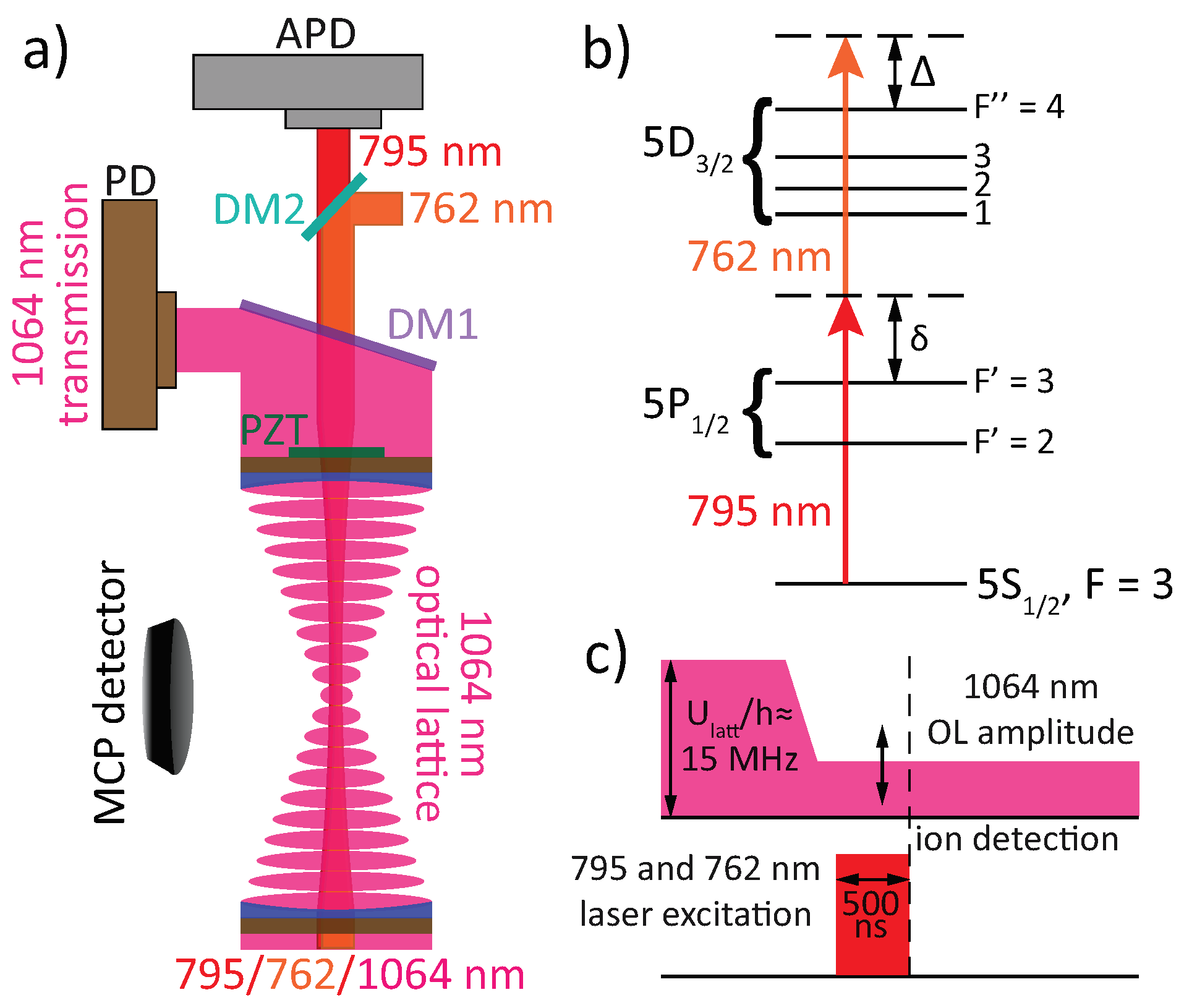
2.2. Experimental Setup
2.3. 1064 nm Power Calibration
2.4. Extracting
3. Results and Discussion
3.1. Determination of
3.2. Discussion of the Result for
3.3. Quantum Interference at
4. Conclusions
Author Contributions
Funding
Data Availability Statement
Acknowledgments
Conflicts of Interest
References
- Ludlow, A.D.; Boyd, M.M.; Ye, J.; Peik, E.; Schmidt, P.O. Optical atomic clocks. Rev. Mod. Phys. 2015, 87, 637–701. [Google Scholar] [CrossRef] [Green Version]
- Bloom, B.J.; Nicholson, T.L.; Williams, J.R.; Campbell, S.L.; Bishof, M.; Zhang, X.; Zhang, W.; Bromley, S.L.; Ye, J. An optical lattice clock with accuracy and stability at the 10−18 level. Nature 2014, 506, 71–75. [Google Scholar] [CrossRef] [PubMed] [Green Version]
- Martin, K.W.; Phelps, G.; Lemke, N.D.; Bigelow, M.S.; Stuhl, B.; Wojcik, M.; Holt, M.; Coddington, I.; Bishop, M.W.; Burke, J.H. Compact Optical Atomic Clock Based on a Two-Photon Transition in Rubidium. Phys. Rev. Appl. 2018, 9, 014019. [Google Scholar] [CrossRef] [Green Version]
- Saffman, M. Quantum computing with atomic qubits and Rydberg interactions: Progress and challenges. J. Phys. B 2016, 49, 202001. [Google Scholar] [CrossRef] [Green Version]
- Morgado, M.; Whitlock, S. Quantum simulation and computing with Rydberg-interacting qubits. AVS Quantum Sci. 2021, 3, 023501. [Google Scholar] [CrossRef]
- Sedlacek, J.A.; Schwettmann, A.; Kübler, H.; Löw, R.; Pfau, T.; Shaffer, J.P. Microwave electrometry with Rydberg atoms in a vapour cell using bright atomic resonances. Nat. Phys. 2012, 8, 819–824. [Google Scholar] [CrossRef]
- Holloway, C.L.; Gordon, J.A.; Jefferts, S.; Schwarzkopf, A.; Anderson, D.A.; Miller, S.A.; Thaicharoen, N.; Raithel, G. Broadband Rydberg Atom-Based Electric-Field Probe for SI-Traceable, Self-Calibrated Measurements. IEEE Trans. Antennas Propag. 2014, 62, 6169–6182. [Google Scholar] [CrossRef] [Green Version]
- Anderson, D.A.; Sapiro, R.E.; Raithel, G. Rydberg Atoms for Radio-Frequency Communications and Sensing: Atomic Receivers for Pulsed RF Field and Phase Detection. IEEE Aerosp. Electron. Syst. Mag. 2020, 35, 48–56. [Google Scholar] [CrossRef]
- Anderson, D.A.; Sapiro, R.E.; Raithel, G. A Self-Calibrated SI-Traceable Rydberg Atom-Based Radio Frequency Electric Field Probe and Measurement Instrument. IEEE Trans. Antennas Propag. 2021, 69, 5931–5941. [Google Scholar] [CrossRef]
- Delone, N.B.; Krainov, V.P. AC Stark shift of atomic energy levels. Physics-Uspekhi 1999, 42, 669–687. [Google Scholar] [CrossRef]
- Gerginov, V.; Beloy, K. Two-photon Optical Frequency Reference with Active ac Stark Shift Cancellation. Phys. Rev. Appl. 2018, 10, 014031. [Google Scholar] [CrossRef] [Green Version]
- Martin, K.W.; Stuhl, B.; Eugenio, J.; Safronova, M.S.; Phelps, G.; Burke, J.H.; Lemke, N.D. Frequency shifts due to Stark effects on a rubidium two-photon transition. Phys. Rev. A 2019, 100, 023417. [Google Scholar] [CrossRef] [Green Version]
- Safronova, M.S.; Arora, B.; Clark, C.W. Frequency-dependent polarizabilities of alkali-metal atoms from ultraviolet through infrared spectral regions. Phys. Rev. A 2006, 73, 022505. [Google Scholar] [CrossRef] [Green Version]
- Topcu, T.; Derevianko, A. Dynamic polarizability of Rydberg atoms: Applicability of the near-free-electron approximation, gauge invariance, and the Dirac sea. Phys. Rev. A 2013, 88, 042510. [Google Scholar] [CrossRef] [Green Version]
- Le Kien, F.; Schneeweiss, P.; Rauschenbeutel, A. Dynamical polarizability of atoms in arbitrary light fields: General theory and application to cesium. Eur. Phys. J. D 2013, 67, 92. [Google Scholar] [CrossRef] [Green Version]
- Marinescu, M.; Sadeghpour, H.R.; Dalgarno, A. Dynamic dipole polarizabilities of rubidium. Phys. Rev. A 1994, 49, 5103–5104. [Google Scholar] [CrossRef]
- Metcalf, H.; van der Straten, P. Laser Cooling and Trapping; Springer: New York, NY, USA, 1999; Volume 3. [Google Scholar]
- Patsch, S.; Reich, D.M.; Raimond, J.M.; Brune, M.; Gleyzes, S.; Koch, C.P. Fast and accurate circularization of a Rydberg atom. Phys. Rev. A 2018, 97, 053418. [Google Scholar] [CrossRef] [Green Version]
- Cardman, R.; Raithel, G. Circularizing Rydberg atoms with time-dependent optical traps. Phys. Rev. A 2020, 101, 013434. [Google Scholar] [CrossRef] [Green Version]
- Grimm, R.; Weidemüller, M.; Ovchinnikov, Y.B. Optical Dipole Traps for Neutral Atoms. Adv. At. Mol. Opt. Phys. 2000, 42, 95–170. [Google Scholar] [CrossRef] [Green Version]
- Weckesser, P.; Thielemann, F.; Hoenig, D.; Lambrecht, A.; Karpa, L.; Schaetz, T. Trapping, shaping, and isolating of an ion Coulomb crystal via state-selective optical potentials. Phys. Rev. A 2021, 103, 013112. [Google Scholar] [CrossRef]
- Cardman, R.; Han, X.; MacLennan, J.L.; Duspayev, A.; Raithel, G. ac polarizability and photoionization-cross-section measurements in an optical lattice. Phys. Rev. A 2021, 104, 063304. [Google Scholar] [CrossRef]
- Nez, F.; Biraben, F.; Felder, R.; Millerioux, Y. Optical frequency determination of the hyperfine components of the 5S1/2-5D3/2 two-photon transitions in rubidium. Opt. Commun. 1993, 102, 432–438. [Google Scholar] [CrossRef]
- Touahri, D.; Acef, O.; Clairon, A.; Zondy, J.J.; Felder, R.; Hilico, L.; de Beauvoir, B.; Biraben, F.; Nez, F. Frequency measurement of the 5S1/2(F = 3)-5D5/2(F = 5) two-photon transition in rubidium. Opt. Commun. 1997, 133, 471–478. [Google Scholar] [CrossRef]
- Hilico, L.; Felder, R.; Touahri, D.; Acef, O.; Clairon, A.; Biraben, F. Metrological features of the rubidium two-photon standards of the BNM-LPTF and Kastler Brossel Laboratories. Eur. Phys. J. Appl. Phys. 1998, 4, 219–225. [Google Scholar] [CrossRef]
- Bernard, J.E.; Madej, A.A.; Siemsen, K.J.; Marmet, L.; Latrasse, C.; Touahri, D.; Poulin, M.; Allard, M.; Têtu, M. Absolute frequency measurement of a laser at 1556 nm locked to the 5S1/2-5D5/2 two-photon transition in 87Rb. Opt. Commun. 2000, 173, 357–364. [Google Scholar] [CrossRef]
- Terra, O.; Hussein, H. An ultra-stable optical frequency standard for telecommunication purposes based upon the 5S1/2→5D5/2 two-photon transition in rubidium. Appl. Phys. B 2016, 122, 27. [Google Scholar] [CrossRef]
- Quinn, T.J. Practical realization of the definition of the metre, including recommended radiations of other optical frequency standards (2001). Metrologia 2003, 40, 103–133. [Google Scholar] [CrossRef]
- Carr, C.; Tanasittikosol, M.; Sargsyan, A.; Sarkisyan, D.; Adams, C.S.; Weatherill, K.J. Three-photon electromagnetically induced transparency using Rydberg states. Opt. Lett. 2012, 37, 3858–3860. [Google Scholar] [CrossRef]
- Thaicharoen, N.; Moore, K.; Anderson, D.; Powel, R.; Peterson, E.; Raithel, G. Electromagnetically induced transparency, absorption, and microwave-field sensing in a Rb vapor cell with a three-color all-infrared laser system. Phys. Rev. A 2019, 100, 063427. [Google Scholar] [CrossRef] [Green Version]
- Duspayev, A.; Han, X.; Viray, M.A.; Ma, L.; Zhao, J.; Raithel, G. Long-range Rydberg-atom–ion molecules of Rb and Cs. Phys. Rev. Res. 2021, 3, 023114. [Google Scholar] [CrossRef]
- Younge, K.C.; Anderson, S.E.; Raithel, G. Adiabatic potentials for Rydberg atoms in a ponderomotive optical lattice. New J. Phys. 2010, 12, 023031. [Google Scholar] [CrossRef]
- Cardman, R.; MacLennan, J.L.; Anderson, S.E.; Chen, Y.J.; Raithel, G.A. Photoionization of Rydberg Atoms in Optical Lattices. New J. Phys. 2021, 23, 063074. [Google Scholar] [CrossRef]
- Snigirev, S.; Golovizin, A.; Tregubov, D.; Pyatchenkov, S.; Sukachev, D.; Akimov, A.; Sorokin, V.; Kolachevsky, N. Measurement of the 5D-level polarizability in laser-cooled Rb atoms. Phys. Rev. A 2014, 89, 012510. [Google Scholar] [CrossRef] [Green Version]
- Terra, O. Absolute frequency measurement of the hyperfine structure of the 5S1/2 – 5D3/2 two-photon transition in rubidium using femtosecond frequency comb. Measurement 2019, 144, 83–87. [Google Scholar] [CrossRef]
- Sheng, D.; Pérez Galván, A.; Orozco, L.A. Lifetime measurements of the 5d states of rubidium. Phys. Rev. A 2008, 78, 062506. [Google Scholar] [CrossRef] [Green Version]
- Aymar, M.; Robaux, O.; Wane, S. Central-field calculations of photoionisation cross sections of excited states of Rb and Sr+ and analysis of photoionisation cross sections of excited alkali atoms using quantum defect theory. J. Phys. B 1984, 17, 993–1007. [Google Scholar] [CrossRef]
- Duncan, B.C.; Sanchez-Villicana, V.; Gould, P.L.; Sadeghpour, H.R. Measurement of the Rb (5 D5/2) photoionization cross section using trapped atoms. Phys. Rev. A 2001, 63, 043411. [Google Scholar] [CrossRef] [Green Version]
- Pohl, T.; Pattard, T.; Rost, J.M. Coulomb Crystallization in Expanding Laser-Cooled Neutral Plasmas. Phys. Rev. Lett. 2004, 92, 155003. [Google Scholar] [CrossRef] [Green Version]
- Viray, M.A.; Miller, S.A.; Raithel, G. Coulomb expansion of a cold non-neutral rubidium plasma. Phys. Rev. A 2020, 102, 033303. [Google Scholar] [CrossRef]
- Schmid, S.; Härter, A.; Denschlag, J.H. Dynamics of a Cold Trapped Ion in a Bose-Einstein Condensate. Phys. Rev. Lett. 2010, 105, 133202. [Google Scholar] [CrossRef]
- Secker, T.; Gerritsma, R.; Glaetzle, A.W.; Negretti, A. Controlled long-range interactions between Rydberg atoms and ions. Phys. Rev. A 2016, 94, 013420. [Google Scholar] [CrossRef] [Green Version]
- Ewald, N.V.; Feldker, T.; Hirzler, H.; Fürst, H.A.; Gerritsma, R. Observation of Interactions between Trapped Ions and Ultracold Rydberg Atoms. Phys. Rev. Lett. 2019, 122, 253401. [Google Scholar] [CrossRef] [PubMed] [Green Version]
- Dieterle, T.; Berngruber, M.; Hölzl, C.; Löw, R.; Jachymski, K.; Pfau, T.; Meinert, F. Transport of a Single Cold Ion Immersed in a Bose-Einstein Condensate. Phys. Rev. Lett. 2021, 126, 033401. [Google Scholar] [CrossRef]
- Hu, Q.Q.; Freier, C.; Sun, Y.; Leykauf, B.; Schkolnik, V.; Yang, J.; Krutzik, M.; Peters, A. Observation of vector and tensor light shifts in 87Rb using near-resonant, stimulated Raman spectroscopy. Phys. Rev. A 2018, 97, 013424. [Google Scholar] [CrossRef] [Green Version]
- Chen, Y.J.; Gonçalves, L.F.; Raithel, G. Measurement of Rb 5P3/2 scalar and tensor polarizabilities in a 1064-nm light field. Phys. Rev. A 2015, 92, 060501(R). [Google Scholar] [CrossRef] [Green Version]
- Neuzner, A.; Körber, M.; Dürr, S.; Rempe, G.; Ritter, S. Breakdown of atomic hyperfine coupling in a deep optical-dipole trap. Phys. Rev. A 2015, 92, 053842. [Google Scholar] [CrossRef] [Green Version]
- MacLennan, J.L. Rydberg Molecules and Excitation of Lattice-Mixed Rydberg States in a Deep Ponderomotive Optical Lattice. Ph.D. Thesis, The University of Michigan, Ann Arbor, MI, USA, 2021. [Google Scholar]
- Chen, Y.J.; Zigo, S.; Raithel, G. Atom trapping and spectroscopy in cavity-generated optical potentials. Phys. Rev. A 2014, 89, 063409. [Google Scholar] [CrossRef] [Green Version]
- Steck, D.A. Rubidium 85 D Line Data, Revision 2021. Available online: http://steck.us/alkalidata (accessed on 8 August 2022).
- Barbier, L.; Pesnelle, A.; Cheret, M. Theoretical interpretation of Penning and associative ionisation in collisions between two excited rubidium atoms. J. Phys. B 1987, 20, 1249–1260. [Google Scholar] [CrossRef]
- Barbier, L.; Cheret, M. Experimental study of Penning and Hornbeck-Molnar ionisation of rubidium atoms excited in a high s or d level (5d ⩽ nl ⩽ 11s). J. Phys. B 1987, 20, 1229–1248. [Google Scholar] [CrossRef]
- Cheret, M.; Barbier, L.; Lindinger, W.; Deloche, R. Penning and associative ionisation of highly excited rubidium atoms. J. Phys. B 1982, 15, 3463–3477. [Google Scholar] [CrossRef]
- Barbier, L.; Djerad, M.T.; Chéret, M. Collisional ion-pair formation in an excited alkali-metal vapor. Phys. Rev. A 1986, 34, 2710–2718. [Google Scholar] [CrossRef] [PubMed]
- Dinneen, T.P.; Wallace, C.D.; Tan, K.Y.N.; Gould, P.L. Use of trapped atoms to measure absolute photoionization cross sections. Opt. Lett. 1992, 17, 1706–1708. [Google Scholar] [CrossRef] [PubMed]
- Bonin, K.D.; Kadar-Kallen, M.A. Theory of the light-force technique for measuring polarizabilities. Phys. Rev. A 1993, 47, 944–960. [Google Scholar] [CrossRef] [PubMed]
- Arora, B.; Sahoo, B.K. State-insensitive trapping of Rb atoms: Linearly versus circularly polarized light. Phys. Rev. A 2012, 86, 033416. [Google Scholar] [CrossRef] [Green Version]
- Taylor, J.R. An Introduction to Error Analysis: The Study of Uncertainties in Physical Measurements, 2nd ed.; University Science Books: Sausalito, CA, USA, 1996. [Google Scholar]
- Anderson, S.E.; Younge, K.C.; Raithel, G. Trapping Rydberg Atoms in an Optical Lattice. Phys. Rev. Lett. 2011, 107, 263001. [Google Scholar] [CrossRef] [Green Version]
- Gross, C.; Bloch, I. Quantum simulations with ultracold atoms in optical lattices. Science 2017, 357, 995–1001. [Google Scholar] [CrossRef] [Green Version]
- Chomaz, L.; Ferrier-Barbut, I.; Ferlaino, F.; Laburthe-Tolra, B.; Lev, B.L.; Pfau, T. Dipolar physics: A review of experiments with magnetic quantum gases. arXiv 2022, arXiv:2201.02672. [Google Scholar]
- Beyer, A.; Maisenbacher, L.; Matveev, A.; Pohl, R.; Khabarova, K.; Grinin, A.; Lamour, T.; Yost, D.C.; Hänsch, T.W.; Kolachevsky, N.; et al. The Rydberg constant and proton size from atomic hydrogen. Science 2017, 358, 79–85. [Google Scholar] [CrossRef] [Green Version]
- Sansonetti, C.J.; Simien, C.E.; Gillaspy, J.D.; Tan, J.N.; Brewer, S.M.; Brown, R.C.; Wu, S.; Porto, J.V. Absolute Transition Frequencies and Quantum Interference in a Frequency Comb Based Measurement of the 6,7Li D Lines. Phys. Rev. Lett. 2011, 107, 023001. [Google Scholar] [CrossRef]
- Brown, R.C.; Wu, S.; Porto, J.V.; Sansonetti, C.J.; Simien, C.E.; Brewer, S.M.; Tan, J.N.; Gillaspy, J.D. Quantum interference and light polarization effects in unresolvable atomic lines: Application to a precise measurement of the 6,7Li D2 lines. Phys. Rev. A 2013, 87, 032504. [Google Scholar] [CrossRef] [Green Version]
- Tully, J.C. Molecular dynamics with electronic transitions. J. Chem. Phys. 1990, 93, 1061. [Google Scholar] [CrossRef]
- Craig, C.F.; Duncan, W.R.; Prezhdo, O.V. Trajectory Surface Hopping in the Time-Dependent Kohn-Sham Approach for Electron-Nuclear Dynamics. Phys. Rev. Lett. 2005, 95, 163001. [Google Scholar] [CrossRef] [PubMed]
- Weber, T.M.; Niederprüm, T.; Manthey, T.; Langer, P.; Guarrera, V.; Barontini, G.; Ott, H. Continuous coupling of ultracold atoms to an ionic plasma via Rydberg excitation. Phys. Rev. A 2012, 86, 020702. [Google Scholar] [CrossRef] [Green Version]
- Anderson, D.A.; Raithel, G.; Simons, M.; Holloway, C.L. Quantum-optical spectroscopy for plasma electric field measurements and diagnostics. arXiv 2017, arXiv:1712.08717. [Google Scholar]
- Ma, L.; Paradis, E.; Raithel, G. DC electric fields in electrode-free glass vapor cell by photoillumination. Opt. Express 2020, 28, 3676–3685. [Google Scholar] [CrossRef] [PubMed]


| Quantity | Value | Source |
|---|---|---|
| 37(3) GW/m/V | This experiment | |
| 687.3(5) a.u. | [57] | |
| −1226(18) a.u. | [47] | |
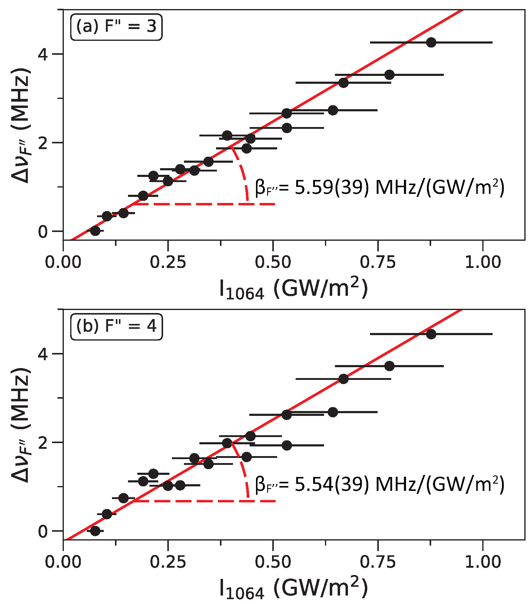
| 5.59(39) MHz/GW/m | This experiment | |
| 5.54(39) MHz/GW/m | This experiment | |
| −505(84) a.u. | Equation (5) | |
| −494(83) a.u. | Equation (5) | |
| −499(59) a.u. | Weighted average |
Publisher’s Note: MDPI stays neutral with regard to jurisdictional claims in published maps and institutional affiliations. |
© 2022 by the authors. Licensee MDPI, Basel, Switzerland. This article is an open access article distributed under the terms and conditions of the Creative Commons Attribution (CC BY) license (https://creativecommons.org/licenses/by/4.0/).
Share and Cite
Duspayev, A.; Cardman, R.; Raithel, G. Dynamic Polarizability of the 85Rb 5D3/2-State in 1064 nm Light. Atoms 2022, 10, 117. https://doi.org/10.3390/atoms10040117
Duspayev A, Cardman R, Raithel G. Dynamic Polarizability of the 85Rb 5D3/2-State in 1064 nm Light. Atoms. 2022; 10(4):117. https://doi.org/10.3390/atoms10040117
Chicago/Turabian StyleDuspayev, Alisher, Ryan Cardman, and Georg Raithel. 2022. "Dynamic Polarizability of the 85Rb 5D3/2-State in 1064 nm Light" Atoms 10, no. 4: 117. https://doi.org/10.3390/atoms10040117