
GRASP: The Future?

1
Mathematical Institute, Oxford University, Oxford OX2 6GG, UK
2
School of Physics, The University of Melbourne, Melbourne, VIC 3010, Australia
*
Authors to whom correspondence should be addressed.
†
These authors contributed equally to this work.
Atoms 2022, 10(4), 108; https://doi.org/10.3390/atoms10040108
Submission received: 14 July 2022
/
Revised: 13 September 2022
/
Accepted: 22 September 2022
/
Published: 2 October 2022
(This article belongs to the Special Issue The General Relativistic Atomic Structure Package—GRASP)
Abstract
:The theoretical foundations of relativistic electronic structure theory within quantum electrodynamics (QED) and the computational basis of the atomic structure code GRASP are briefly surveyed. A class of four-component basis set is introduced, which we denote the CKG-spinor set, that enforces the charge-conjugation symmetry of the Dirac equation. This formalism has been implemented using the Gaussian function technology that is routinely used in computational quantum chemistry, including in our relativistic molecular structure code, BERTHA. We demonstrate that, unlike the kinetically matched two-component basis sets that are widely employed in relativistic quantum chemistry, the CKG-spinor basis is able to reproduce the well-known eigenvalue spectrum of point-nuclear hydrogenic systems to high accuracy for all atomic symmetry types. Calculations are reported of third- and higher-order vacuum polarization effects in hydrogenic systems using the CKG-spinor set. These results reveal that Gaussian basis set expansions are able to calculate accurately these QED effects without recourse to the apparatus of regularization and in agreement with existing methods. An approach to the evaluation of the electron self-energy is outlined that extends our earlier work using partial-wave expansions in QED. Combined with the treatment of vacuum polarization effects described in this article, these basis set methods suggest the development of a comprehensive ab initio approach to the calculation of radiative and QED effects in future versions of the GRASP code.
1. Introduction
Electronic structure theory has driven the development of atomic, molecular and solid state physics for almost a century. The nonrelativistic self-consistent field model pioneered by Douglas Hartree in the pre-computer era formed the foundations of atomic structure theories and a theoretical understanding of the structure of the Periodic Table of the elements. This model was incorporated into atomic structure computer codes which have remained under constant development for more than half a century. These codes include the nonrelativistic ATSP and relativistic GRASP programs that are based on the multiconfigurational Hartree–Fock formalism described in the well-known 1957 lectures by Hartree [1].
The development of relativistic electronic structure theories has been motivated by the need to incorporate physical effects not described by the Schrödinger equation, which are usually most evident in systems containing heavy elements. In this article, we restrict our attention to electronic structure models based on the four-component Dirac equation for mean-field potentials [2,3], with subsequent treatment of many-body effects using perturbative, configurational or coupled-cluster expansions, or the two-particle reduced density matrix approach. The formalisms for these computational approaches are equally applicable to the determination of atomic and molecular structures and are widely employed in existing computational codes.
The developers of the GRASP codes, of which GRASP2018 [4,5] is the most recent release, have been motivated both by the experimental demands of atomic spectroscopy and by the desire to formulate computational methods that are consistent with the underlying theory of quantum electrodynamics (QED), achieving both accuracy and completeness. The structure of the code is sketched in Section 2. It has become a widely-used tool in atomic spectroscopy, with many applications in solar, stellar and plasma physics and as a platform for the exploration of relativistic, many-body and QED effects, especially in systems containing heavy elements. It has also been used to gain insights into molecular and solid state physics, in investigations of particle physics beyond the Standard Model, and in recent searches for the experimental signatures of dark matter.
The relativistic molecular electronic structure code BERTHA [6,7] has been developed within the same theoretical framework as GRASP. These common foundations are described in detail in [8] and are summarized in Section 3. Potential synergies between GRASP and BERTHA that exploit their common structures and shared formulation form the basis of this article. Both codes generate numerical four-component solutions of the Dirac equation which define distinct non-interacting fields of electrons or positrons. Furry provided a covariant derivation of the bound-state interaction picture of QED within the Feynman-Dyson formalism [9]. Charged particles in the Furry picture interact only through coupling to the Maxwell field, emitting and absorbing virtual photons. Both GRASP and BERTHA, which assume that the exchange of energy involves single photons, represented by Coulomb, Breit or other interactions, are computational implementations of the Furry picture. Radiative corrections, electron self-energy and vacuum polarization effects, involve one-photon exchanges between the uncoupled electron and positron fields.
In common with most research in relativistic electronic structure theory (see, for example [10,11,12,13,14,15,16], the development of GRASP and BERTHA has focussed on the construction of positive-energy bound-states and many-body corrections that exclude explicit reference to the negative-energy sector of the spectrum. This approach does not exclude consideration of QED corrections, but restricts their calculation to the evaluation of bound-state expectation values of effective interaction operators, examples of which have been implemented in GRASP. In Section 3.3.3, we consider a new class of four-component basis set that is consistent with the Furry picture, the charge-conjugation symmetries of the free-particle Dirac equation and the relativistic Gaussian basis set technologies that we have developed for molecular physics and quantum chemistry. We demonstrate in Section 4 that this basis set is able to calculate the vacuum polarization effects attributed to the Wichmann-Kroll interaction from a first-principles implementation of QED. This is achieved without recourse to the use of effective potentials or the machinery of regularization that is usually invoked to handle divergences in QED [17]. This formulation echoes our approach to the calculation of the electron self-energy [18,19,20] and the work of Lindgren and collaborators [21,22], but is based on quite different computational methods that have evolved through our work on molecular structure. We conclude by suggesting that these basis set methods may be usefully employed in future developments of GRASP.
2. Building Atomic Structure Programs
The software repository [5] of the CompAS (Computational Atomic Structure) collaboration [23] supplies the nonrelativistic ATSP and the relativistic GRASP programs, both based on multiconfiguration Hartree–Fock ideas expounded in Hartree’s 1957 lectures [1]. Bound electron orbitals, the building blocks of nonrelativistic configurational states (CSF) in ATSP have the familiar form:
in spherical polar coordinates, where are orbital angular momentum quantum numbers and the spin projection. The label n enumerates successive bound orbitals of this symmetry, replaced by the energy, , above threshold for ionization to the continuum. We shall refer to the orbitals labelled as the -subshell, with the common radial factor .
In relativistic programs like GRASP these are replaced by 4-component spinors [2,8]
where the 2-component coupled spin–orbit function is
In this case each -subshell consists of orbitals, with common radial functions . It is often convenient to replace the label with the more familiar set with , as , and in the limit .
These orbital functions are the building blocks for many-electron wave functions. The simplest is the Slater determinant
that vanishes if more than one electron orbital is assigned the same state label or the same location , thus ensuring that no orbital has more than one occupant in accordance with Pauli’s exclusion principle. GRASP programs classify configurational states (CSF)—notionally a linear combination of Slater determinants—in -coupling: denotes an n-electron CSF with total angular momentum quantum numbers , and parity ; includes all additional information, in particular the angular momentum coupling scheme, needed to specify uniquely using Racah’s theory of angular momentum ([8], Sections 6.6–6.8). CSF in ATSP, , are formed in much the same way. The atomic state functions, ASFs, are linear combinations of CSFs of the same symmmetry, .
Given estimates of the orbitals, we can construct matrix elements of the Hamiltonian of an N-electron atom with respect to the CSFs . Diagonalization of generates ASFs and ASF energies with the same spectroscopic classification.
The GRASP orbital equations are described in ([8], Chapter 7). Here, as in [8], we adopt Hartree atomic units for which , and . We also adhere to the notational conventions of [8], in that the Dirac matrices and are employed when discussing computational implementations of relativistic electronic structure theory, and the matrices appear when discussing the formulation of the theory within quantum electrodynamics. The correspondence between these notations and their properties are discussed in ([8], Appendix A.2) and summarized by the relations and . If the electron mass, , and charge, e, appear in formulae it is to emphasise dimensionality, but it is implicitly understood that they should be assigned unit value. The (unquantized) multi-configurational Dirac-Hartree–Fock–Breit (MCDHFB) Hamiltonian for an N-electron atom with point charge nucleus Z has the form
where
is the Dirac Hamiltonian for electron i. The electron-electron interaction potential is just the classical Coulomb potential, augmented by the Breit interaction. A standard variational argument generates coupled sets of integro-differential equations, one for each participating subshell A, of the form ([8], Section 7.3)
The potential energy is the sum of the nuclear Coulomb potential energy and, the ‘direct’ (or classical) Coulomb repulsion from subshells . The exchange repulsion energy from other electrons in subshell A is also included in . The quantities on the right are ‘exchange’ potentials together with any Lagrange multipliers, , required to preserve orbital orthonormality. Each such equation, given estimates of the interaction with other subshells, provides an estimate of . They can be used to modify the interaction potentials for the next iteration of the equations until all orbitals have stabilized to agreed precision.
Equation (7) recognizes only subshells containing at least one electron. Other one-electron states of that symmetry are ignored, in particular the negative-energy solutions representing positrons in the atomic field. These are never calculated in MCDHFB models but, though ignored, they are implicitly part of the model.
Numerical methods to solve Equation (7) in GRASP and similar programs in the Hartree tradition are mostly based on finite differences although a number of recent programs have used B-spline expansions. Relativistic molecular calculations require basis set methods proposed by Roothaan [24] and Hall [25]. This approach has rarely been used for atomic problems, and there were many failed attempts to construct 4-spinor basis sets before the need for kinetic matching of the two radial components was established ([8], Section 5.7). The BERTHA relativistic molecular package [6,7] relies on the atomic kinetically-matched spinor basis sets described in Section 3.3.1. Four-spinor basis set algorithms automatically generate both electron and positron wave functions; the positron solutions play no part in atomic and molecular structure. Calculation of additional contributions suggested by QED require a computational scheme with further symmetry constraints on the 4-spinor basis functions to balance the representation of electrons and positrons.
3. QED of Atoms and Molecules
3.1. Relativistic Wave Equations
The early history of relativistic wave equations is well documented by, for example, the books [26,27,28]. Dirac’s ‘negative energy states’ and their stop-gap ‘hole theory’ [29,30,31,32,33] made it impossible to regard their relativistic wave equation as describing motion of a single particle in the manner of the Schrödinger equation, inspiring the development of quantum field theory. The unquestioned acceptance of the physical reality of Dirac’s ‘hole theory’ created major problems in the design of mathematical and computational algorithms for relativistic atomic and molecular structure. Variational methods of nonrelativistic quantum mechanics are routinely justified by the existence of a finite lower bound to the atomic or molecular Hamiltonian, so that iterative decreasing sequences of level energies may converge to a limit according to Cauchy’s general principle of convergence. The spectra of Dirac Hamiltonians are infinite above and below leading to an extensive literature regarding problems associated with the application of the linear variation method to relativistic electronic structure theory. A review of this literature and a discussion of both the linear variation method and the application of min-max principles to relativistic electronic structure problems may be found in ([8], Section 5.5). This is where relativistic spinor adaptations of the ideas of Roothaan [24] and Hall [25] and an understanding of their symmetry structure came to the rescue.
3.2. Quantized Electron and Positron Fields
This section follows ([28], Section 14.1). The Dirac equation for free particles (in atomic units) is
We can think of this as a field equation, interpreting as an operator on the states of the Dirac field rather than providing particle wave functions. Label the states of the Dirac field , where the index n runs over all possible field modes, with the vacuum state . We define the wave functions such that
as solutions of the equations
Invariance with respect to time translation allows us to write
for positive and negative energy modes, respectively, so that the -dependent amplitudes satisfy the time-independent Dirac equations
Expand the field operators in the form
with anticommuting creation and annihilation operators such that
All other anticommutators vanish. If we set the equal-time anticommutator of the field operators to be
where ; then
so that the complete spectrum of the Dirac free particle field operator has both positive- and negative-energy solutions. The formalism implies that electrons and positrons obey Fermi statistics: there can be only one electron in state r or positron in state s. In all physically realistic models, the electron and positron spectra are quite distinct, although their wave functions satisfy the same Dirac equation. This formalism makes it possible to think of separate electron and positron fields. Then
are, respectively, the total number and total energy of the quanta of the electron and positron fields. The combined totals are
This construction can also be used with minimal coupling to an external electromagnetic field, , so that
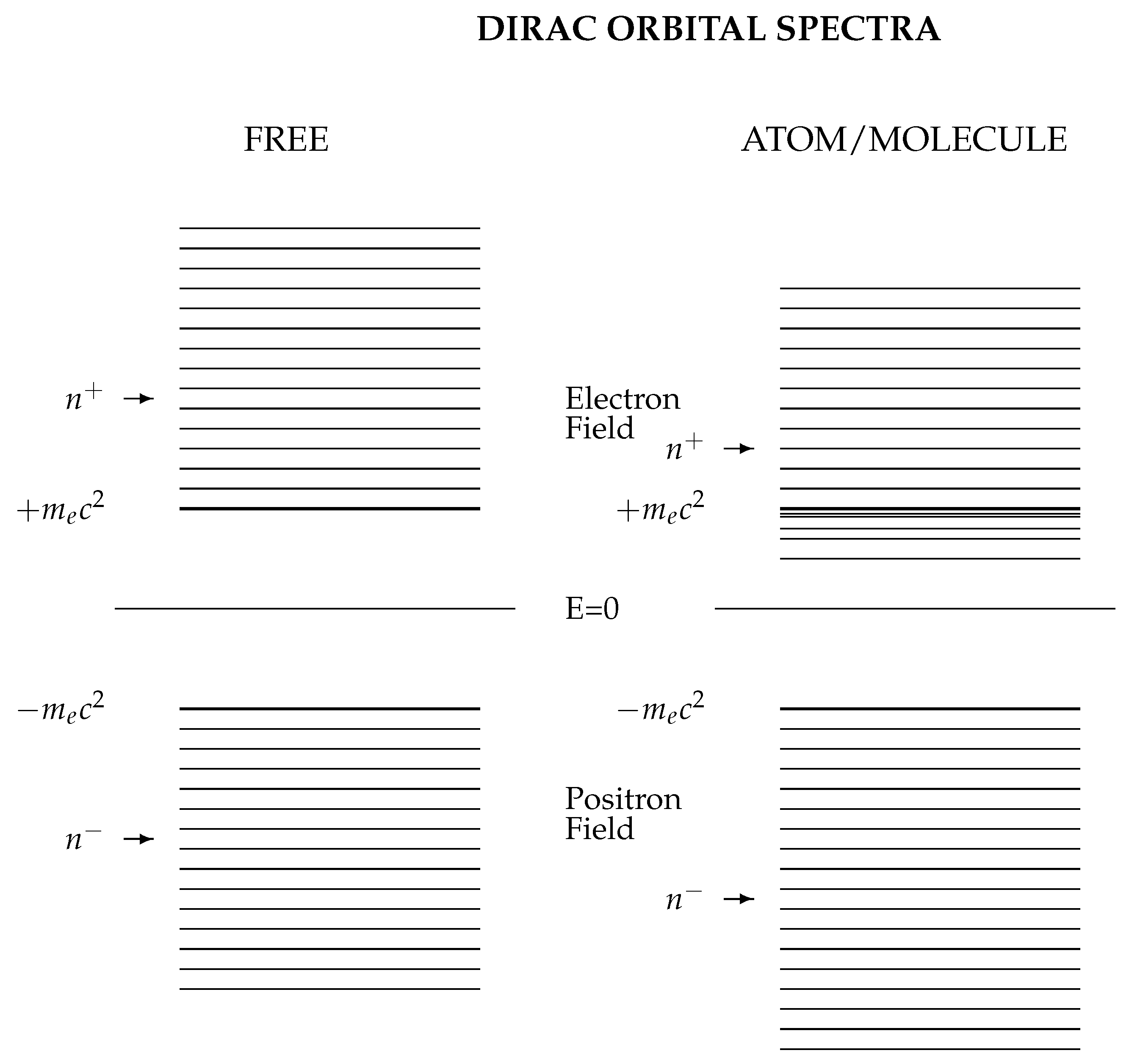
The electron field and the positron fields are again in separate domains. The charge conjugation symmetry is broken in an atomic environment as shown schematically in Figure 1.
Quantization of the electron and positron fields is independent of the particular method of solution of the Dirac equation. Figure 1 illustrates schematically the symmetry of the free fermion levels and about the relativistic energy zero. The charge conjugation operator, C of Section 3.3.2, sets up a bijective mapping between the and energy states of free fermions. This symmetry is broken in the atomic or molecular environment; all realistic physical models identify separate electron and positron domains, which we can think of as defining separate quantum fields although the wave functions are solutions of the same Dirac equation.
3.3. Basis Set Spinor Expansions
The formalism in current use for solving relativistic atomic and molecular structure problems using a linear combination of spinor basis functions is surveyed in ([8], Sections 5.6–5.11). An orbital a in subshell A having the structure (2) is approximated by
where labels the large- and small-component basis spinors, , which in a molecule may be centred on more than one nucleus. The time-independent Dirac Hamiltonian for an electron can be written as in (11)
where the potential energy may include contributions from interactions with other electrons and nuclei. We can now form a Rayleigh quotient by taking the expectation of with respect to :
where the elements of the N-vectors are the expansion coefficients of (18),
The matrices have elements
so that the matrix is Hermitian. The Rayleigh-Ritz variational method gives Galerkin equations
This generalized eigenvalue equation for eigenvalues and eigenfunctions requires basis 4-spinors to have specific relations between their components to give physically useful results. Following (2), we assume
The kinetic matching restriction ([8], Section 5.7) of the radial components
ensures that the matrix reduces to the corresponding Schrödinger matrix with respect to the radial functions for positive-energy states in the nonrelativistic limit. More specifically, this construction—we refer to ([8], Chapter 5) for the details—gives the nonrelativistic kinetic energy matrix ([8], Equation (5.7.13)).
so that (21) reduces to the matrix Schrödinger equation
where is the eigenvalue relative to the nonrelativistic zero of energy. Note that kinetic matching is not a direct relativistic effect. It is a consequence of the internal structure of the Dirac operator, essential for ensuring correct behaviour in the nonrelativistic limit. A similar argument reveals that (23) holds with a change of sign for negative energy solutions, leading to the Schrödinger equation with the repulsive potential for low energy positrons with energy . Successful types of kinetically matched spinor basis functions are listed in ([8], Sections 5.8–5.10) along with numerical examples.
3.3.1. KG-Spinors
The fact that the upper (“large”) radial component of a 4-spinor may be of any form used in nonrelativistic atomic models defines the class of K-spinors (K denotes ‘kinetically matched’) in which the radial components are related by (23). We consider only the Gaussian (KG-spinor) sets (G denotes ‘Gaussian function’), from which the BERTHA relativistic molecular program [6] is built:
where the exponents are with suitable chosen parameters that may depend on . From (23), the lower components are
where are arbitrary constants, chosen to enforce normalization. KG-spinors have been shown to give excellent results for atomic and molecular structure and properties but they lack the symmetry needed to give a balanced representation of negative-energy states.
3.3.2. Charge Conjugation
The charge conjugation matrix C sets up a bijective mapping between the elements of the domains of free electrons and positrons. In the Dirac representation, this matrix is given by ([8], Appendix A.2):
where is Dirac conjugation. The asterisk denotes complex conjugation, and superscript t denotes vector transposition. Minimal coupling of a particle with charge q to an external electromagnetic field replaces (8) by
A simple calculation shows that
so that charge conjugation reverses the sign of the particle’s charge. The expectation value of an operator is given by
so that for free particles we have
These electron/positron symmetry relations are broken by interaction with other particles in atoms and molecules. Figure 1 compares the spectrum of the Dirac operator for free particles on the left, with a typical atomic potential on the right, generated using a basis set which respects free particle charge conjugation. The free spectrum is symmetric about energy , while the atomic potential lowers all eigenvalues, introducing bound states and making .
Atomic and molecular structure calculations write the Dirac Hamiltonian in the form
so that for particles of charge q
The standard 4-spinor in spherical coordinates with real radial amplitudes has the form
applying (28) gives the charge conjugate spinor
3.3.3. CKG-Spinors
The charge conjugation operator discussed in Section 3.3.2 imposes a symmetry on four-component Dirac spinors under the transformation . A complete set that satisfies charge conjugation symmetry must consist of all spin-angular symmetry types, and contain elements classified by positive or negative energy. In a Gaussian representation, we denote such a basis the CKG set (C denotes ’charge conjugate’), which expands an arbitrary Dirac spinor through the relation:
where denotes positive- and negative-energy, respectively, and setting ,
with normalization constants . For a given symmetry-type, , we choose a Gaussian basis set for the large components of positive energy free-particle states, from which the corresponding small component functions are derived by application of the free-particle Dirac equation, which fixes the relative amplitudes of the components. For positive energies (), the explicit forms of the radial components are
The behaviour of these functions at small r resembles that of the analytic solutions of the radial free-particle functions, which are proportional to r times a spherical Bessel function, ([8], Equation (3.2.24)). Coincidently, this is also consistent with the small r behaviour of Dirac spinors for finite nuclear models, for which the potential approaches a constant value.
With these choices for positive-energy radial basis spinors, charge conjugation symmetry dictates the construction of negative-energy radial basis functions to be:
The parameter , corresponds to the magnitude of the average free-particle energy. In the so-called “dual kinetic balance” basis [12], this parameter is simply set to , on the grounds that we are mainly interested in positive-energy bound-states. As high-energy states play a significant role in QED correction calculations, we choose
where
The normalization constants, , are chosen so that
for all valid and m.
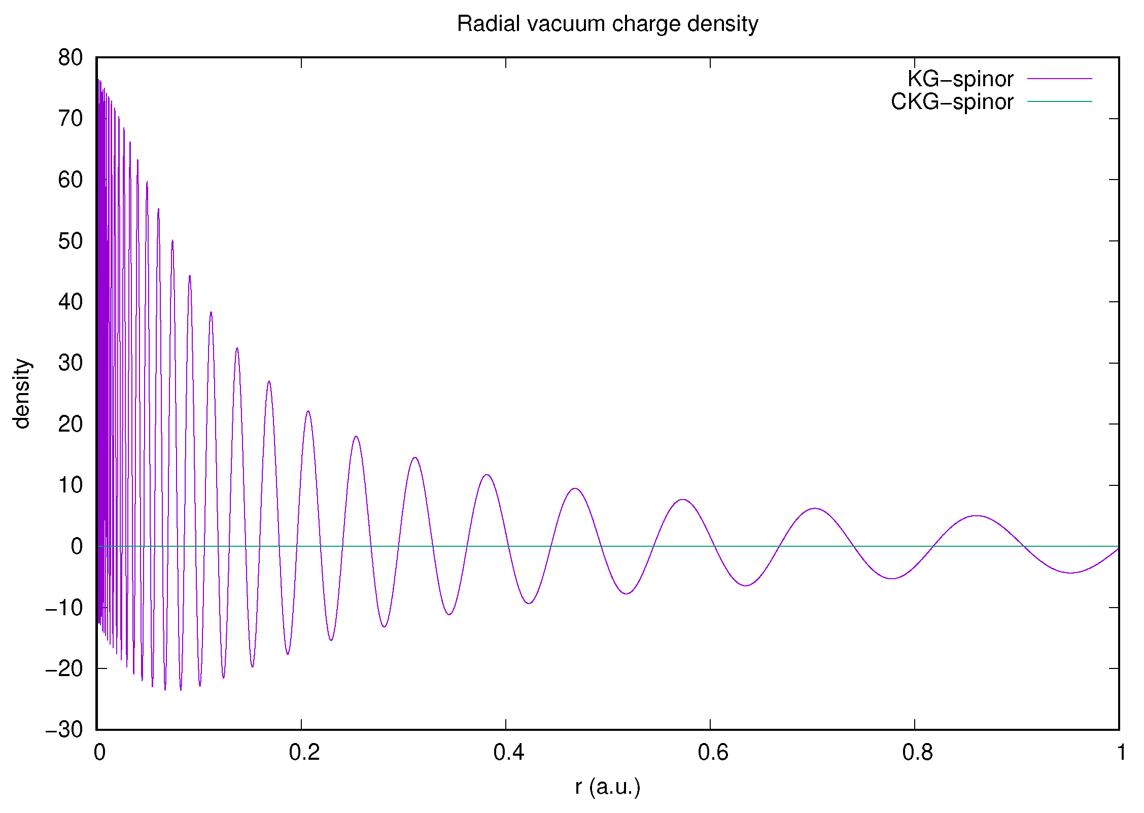
Figure 2 vividly illustrates the necessity of charge conjugation symmetry in a calculation of the contribution to the vacuum charge density. The rapid oscillations of the KG-spinor radial density integrate to zero, whilst the CKG-spinor calculation radial densities cancel within rounding errors for all radii by construction. This ensures charge and parity conservation in interaction matrix elements.
Table 1 reports eigenvalues of a test calculation on the hydrogenic ion Hg obtained with a large CKG-spinor basis. The exponents for all values of were with . The table reports only the first three numerical eigenvalues of each symmetry together with the lowest exact analytic eigenvalue. The first two columns agree to 10 decimal places for all with the minor exception of the first two lines . The atomic symmetry requires that point-nuclear hydrogenic eigenvalues are degenerate for states that share the same and quantum numbers. We find 12 significant figure agreement between the and eigenvalues. This pairwise numerical agreement persists across all symmetry-types considered in Table 1 up to ; the numerical values of the degenerate pairs of energies coincide with the corresponding Dirac-Sommerfeld eigenvalues.
4. QED Corrections
Vacuum Polarization
A long-standing ambition has been to evaluate numerically on the fly the contribution of vacuum polarization to orbital energies for each atomic state. CKG-spinors defined in Section 3.3.3 make this possible. This is because we can diagonalize the Dirac Hamiltonian
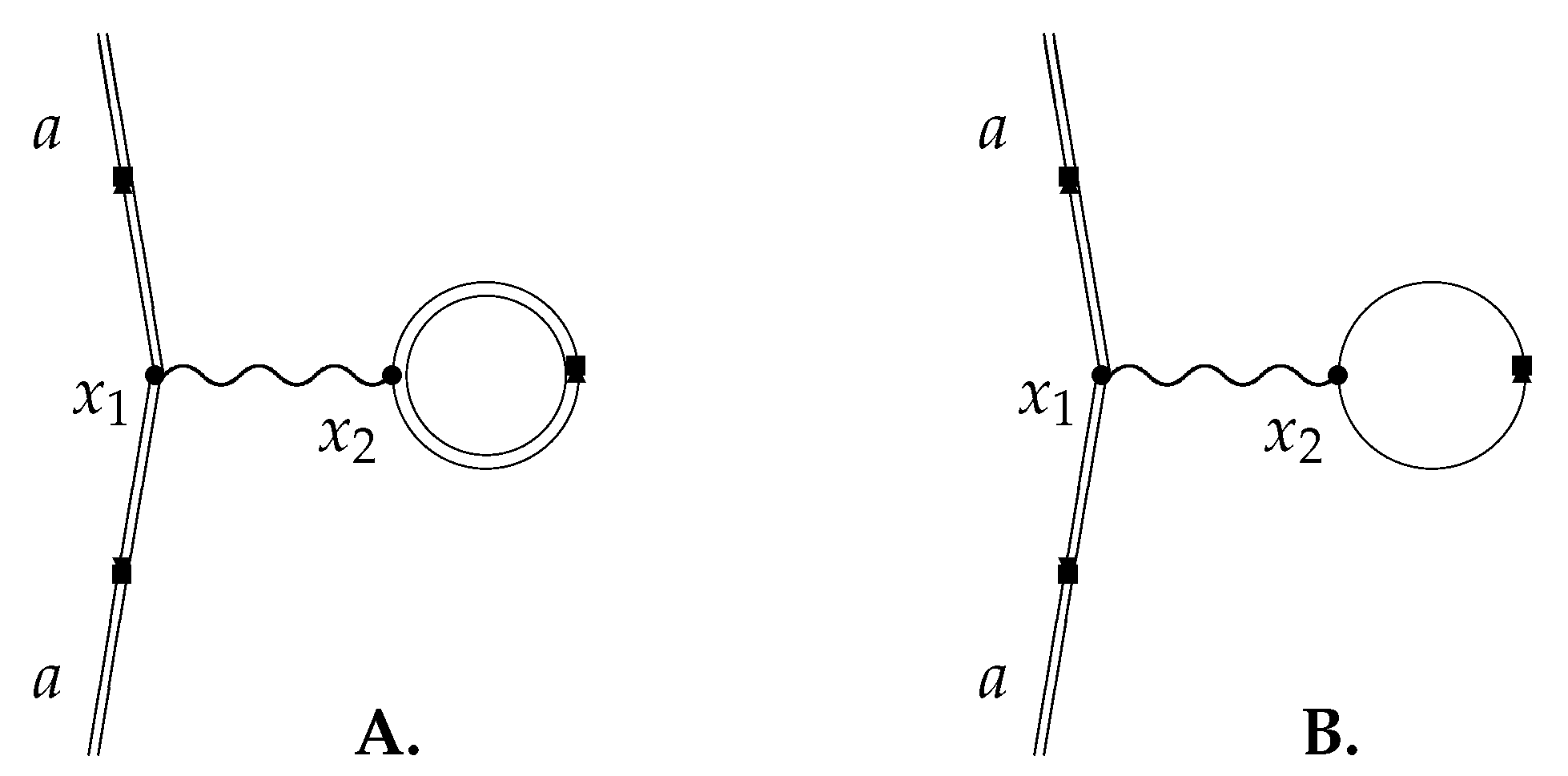
for all Z in terms of a common basis, simplifying evaluation of the matrix elements appearing in Equations (42) and (43) below. The principle of this calculation was demonstrated by Persson et al. [21] who used a similar technology based on partial wave expansion to evaluate the Wichmann-Kroll potential [34,35]. They started from the Feynman diagram, Figure 3, expanding the photon propagator in partial waves ([21], Equation (2.6)).
where denotes the spherical tensor of order l associated with the coordinate labelled i. Any vacuum polarization acting on the electron in atomic orbital a is due to the closed loop in which electrons circulate in one direction and positrons in the other. In Figure 3B the currents cancel by charge conjugation symmetry so that the photon has zero energy [36]; the external field breaks the charge conjugation symmetry of electrons and positrons as illustrated in Figure 1 so that the exchanged photon in Figure 3A has a finite energy. (Schweber [37] makes this point in a review of the Furry Picture). Equation (42) can be simplified giving
where the index t in (42) has been replaced by n. The summation over n includes the complete set of radial functions for each . The case applies to freely moving electrons, and it is easy to show that pairs of matrix elements related by charge conjugation symmetry cancel. This symmetry is broken when .
Figure 2 has already demonstrated that the CKG-spinor result for the zero potential term, , is consistent with Furry’s theorem. We can also use the CKG-spinors to evaluate the one-potential term:
using the free particle Dirac Hamiltonian, , to evaluate the kets and free particle eigenvalues . CKG-spinor evaluation of the matrix elements is straightforward. Alternatively, we can use free electron partial waves whose radial amplitudes are proportional to spherical Bessel functions, giving matrix elements proportional to the vertex integrals [19].
Table 2 compares partial wave contributions to the vacuum polarization in Hg with a point nucleus. The first column is the CKG-spinor contribution from (43) using atomic spinors with . Column 2 shows the corresponding unrenormalized one-potential contribution from (44) with the generated in the same CKG-spinor basis. Following [21], we interpret the difference in the last column as the contribution of Wichmann-Kroll and higher order contributions. Table 3 compares the values of the Wichmann-Kroll contribution for a range of values of Z with the corresponding CKG-spinor calculation. , column 2, is the expectation of the WK-potential defined in [35] integrated over the analytic charge density. The value of for in the last column is extrapolated from the sum in Table 2.
We have not yet been able to make comparisons with extensive calculations such as those of Sapirstein and Cheng [38], who used a coordinate space formalism to calculate vacuum polarization energies for hydrogenic ions with finite size nuclei and principal quantum numbers . They also calculated results for lithium-, sodium- and copper-like ions using Kohn-Sham potentials and first-order screening corrections. These are brute force computations. They found it necessary to use an extremely fine radial grid of up to 50,000 points when calculating electron wave functions to control the accuracy of the photon energy integration, where they encounter numerical instabilities giving unphysical behaviour at very high energies or greater.
5. Electron Self-Energy
There seems no reason why charge symmetric CKG-spinors should not be equally useful in calculating the electron self-energy correction [39,40] to atoms and molecules. The partial wave renormalization approach was developed in [18,19] and, with rather different technology, in [21]. The partial wave expressions to be evaluated for the self-energy of a bound orbital a can be reduced to the general form
where the sum over intermediate virtual states runs over the complete Dirac spectrum. The integrand is finite for each , but the partial wave sum over diverges logarithmically whether for free () or bound () sums ([18], Table 1). We write when the intermediate states are free, , and for . The divergent sum , the renormalization counter term, is usually interpreted as already forming part of the observed mass of the electron. Partial wave renormalization amounts to calculating the convergent sum , where ([18], Table 2).
The use of CKG-spinors for self-energy has still to be investigated. The results of [18,19] for used a Wick rotation, , for the configuration space propagator in (45) similar to that used by Sapirstein and Cheng [38] in their work on vacuum polarization. The counter terms treated the bound state as a wave packet superposition of free states of the same symmetry : , so that the matrix elements in the numerator of (45) are proportional to the free electron vertex integrals [20]. The different algorithms all give similar accuracy.
6. Conclusions
QED was formulated [26,27,28,37], when computers were in their infancy and the most advanced computational aids were hand or electric calculators. Relativistic atomic structure programs like GRASP initially adapted algorithms in the 1960s ([3], Table 3) on lines proposed in Hartree’s 1957 lectures [1]. The symmetry structure of Dirac spinors on which GRASP is built [2,8], not yet fully understood in 1957, would not have been possible without the fundamental work of Racah [41,42,43] on quantum theory of angular momentum. Deeper understanding of the symmetry structure of spinor basis sets, developed over the last 30 years, along with advances in computer power and computational software, have motivated the fusion of computational methods from atomic and molecular physics and quantum electrodynamics discussed in this article.
Those familiar with quantum field theory will no doubt question why it is possible to perform calculations of radiative corrections in atoms without encountering the endemic infinities of perturbative QED. Weinberg ([28], Section 1.3) discusses the historic ‘problem of infinities’, noting that major progress on QED in the late 1940s required confidence in renormalization techniques. Similarly ‘Renormalization theory is a complicated conceptual system. …The renormalization procedure can be viewed as a technical device for circumventing—and discarding—the infinite results that occur in perturbative calculations in quantum field theory.’ ([27], p. 595) The reliance on regularization and renormalization has largely restricted serious attempts to calculate radiative corrections without expansion in powers of to one- or two-electron systems. Spectroscopic applications need reliable data for many-electron atoms and ions beyond the first rows of the Periodic Table. GRASP and other programs rely on approximate formulae for self-energy and vacuum polarization based on hydrogenic calculations or effective potential approaches.
The complete reconciliation of conventional QED with the approach we have presented in this article and in our earlier work on the self energy [18,19] poses some open questions. There are clues: it is natural to use central field orbitals in atomic and molecular calculations, so that partial wave amplitudes at the vertices of Feynman diagrams are constrained by conservation of 3-momentum, angular momentum and parity as discussed in [20]. In the calculations of vacuum polarization reported here, and of the self-energy in [18,19], the Feynman diagrams are evaluated as partial wave expansions. Each term in these expansions is finite, and calculated without the use of any form of regularization. In the case of the self-energy, a partial wave mass-renormalization counter-term was introduced that renders the calculation of the physical effect finite, and in agreement with the results of conventional QED and experiment. We have demonstrated that the calculation of the higher-order terms in the vacuum polarization may also be achieved without regularization using the CK-basis, by subtracting corresponding terms in the partial wave expansions defined by Equations (43) and (44). This computational procedure is successful because the zero-potential term, and all higher-order terms involving an even number of external field interactions, vanish. This is a formal requirement of Furry’s theorem, but is not satisfied for all choices of basis set. The kinetically-balanced KG-basis set fails this fundamental test, as shown in Figure 2 and in results presented in [44]. The CKG-basis set passes this test by construction, so only physically meaningful contributions participate in the calculation of physical effects. Strong numerical cancellations are observed between the partial wave contributions in Table 2, which would be overwhelmed by any numerical failure of Furry’s theorem in the zero-potential term.
Our calculations of the leading-order self energy in [18,19] include external field contributions to all orders in , but the treatment of vacuum polarization discussed here includes only contributions of order and higher. The missing part of the vacuum polarization of order is represented by the expectation value of the Uehling potential. This well-understood effective potential incorporates charge renormalization and is conventionally derived using some form of regularization to tame the divergences that arise in its derivation. Our treatments of the self-energy and vacuum polarization would appear to be more symmetric and mutually complementary if the formally divergent part of the one-potential term, Equation (44), could be identified and eliminated within the partial wave expansion. It is an implicit assumption of our analysis, and of earlier work [21], that Equations (43) and (44) each contain the finite parts of the Uehling interaction and the divergent parts requiring renormalization. By the same reasoning, the sum of the differences for each partial wave results in a convergent series of finite, higher-order terms, but excludes the effects of the Uehling potential. A detailed analysis of the formulation of the vacuum polarization effect in configuration-space is presented in [17]. We are yet to develop this analysis to achieve an all-order treatment of vacuum polarization within the CKG-basis representation, though the calculation of the higher-order terms represents significant progress in that direction.
Since the calculation of bound-state matrix elements of the Uehling potential is readily achieved to high accuracy using any of the conventional methods of atomic physics, the combination of our methods for higher-order effects with a conventional calculation of the leading-order Uehling effect already offers a new computational treatment of QED effects. The unified approach that we have explored in this article points, however, to the development of a first-principles treatment mean-field, many-body and radiative effects within a common basis set and without the use of the QED machinery of regularization.
The adoption of a pragmatic point of view might suggest that the use of a patchwork of computational approaches in relativistic electronic structure theory currently achieves the accuracy required by experimental data in most practical applications. One should never forget, however, that a change of viewpoint, motivated by aesthetics, physical transparency or appeals to fundamental symmetries, may suggest new and better ways of doing things.
Author Contributions
Conceptualization, I.G. and H.Q. All authors have read and agreed to the published version of the manuscript.
Funding
This research received no external funding.
Institutional Review Board Statement
Not applicable.
Informed Consent Statement
Not applicable.
Data Availability Statement
Not applicable.
Acknowledgments
This paper, a work in progress, is the outcome of many years of discussion between the authors on the use of basis set methods in atomic and molecular structure. HMQ did the calculations.
Conflicts of Interest
The authors declare no conflict of interest.
References
- Hartree, D.R. The Calculation of Atomic Structures; John Wiley & Sons, Inc.: New York, NY, USA, 1957. [Google Scholar]
- Grant, I.P. Relativistic self-consistent fields. Proc. R. Soc. A 1961, 262, 555–576. [Google Scholar] [CrossRef]
- Grant, I.P. Relativistic calculation of atomic structures. Adv. Phys. 1970, 19, 747. [Google Scholar] [CrossRef]
- Froese Fischer, C.; Gaigalas, G.; Jönsson, P.; Bieroń, J. GRASP2018-A Fortran 95 version of the General Purpose Relativistic Atomic Structure Package. Computer Phys. Commun. 2018, 237, 183–187. [Google Scholar]
- Available online: https://github.com/compas (accessed on 1 June 2022).
- Quiney, H.M.; Skaane, H.; Grant, I.P. Relativistic calculation of electromagnetic interactions in molecules. J. Phys. B At. Mol. Opt. Phys. 1997, 30, L829. [Google Scholar] [CrossRef]
- Belpassi, L.; de Santis, M.; Quiney, H.M.; Tarantelli, F.; Storchi, L. BERTHA: Implementation of a four-component Dirac-Kohn-Sham relativistic framework. J. Chem. Phys. 2020, 152, 164118. [Google Scholar] [CrossRef]
- Grant, I.P. Relativistic Quantum Theory of Atoms and Molecules: Theory and Computation; Springer Science and Business Media, LLC: New York, NY, USA, 2007. [Google Scholar]
- Furry, W.H. On bound states and scattering in positron theory. Phys. Rev. 1951, 81, 115. [Google Scholar] [CrossRef]
- Desclaux, J.-P. Relativistic Dirac-Fock expectation values for atoms Z = 1 to Z = 120. At. Data Nucl. Data Tables 1973, 12, 311–406. [Google Scholar] [CrossRef]
- Johnson, W.R.; Sapirstein, J. Computation of second-order many-body corrections in relativistic atomic systems. Phys. Rev. Lett. 1986, 57, 1126. [Google Scholar] [CrossRef]
- Shabaev, V.M.; Tupitsyn, I.I.; Yerokhin, V.A.; Plunien, G.; Soff, G. Dual kinetic balance approach to basis set expansions for the Dirac equation. Phys. Rev. Lett. 2004, 93, 130405. [Google Scholar] [CrossRef] [Green Version]
- Dyall, K.G.; Faegri, K. Introduction to Relativistic Quantum Chemistry; Oxford University Press: Oxford, UK, 2007. [Google Scholar]
- Zatsarinny, O.; Froese-Fischer, C. DBSR_HF: A B-spline Dirac-Hartree-Fock program. Comput. Phys. Commun. 2016, 202, 287–303. [Google Scholar] [CrossRef] [Green Version]
- Liu, W. Essentials of relativistic quantum chemistry. J. Chem. Phys. 2020, 152, 180901. [Google Scholar] [CrossRef] [PubMed]
- Saue, T.; Bast, R.; Perero Gomes, A.S.; Jensen, H.A.; Visscher, L.; Aucar, I.A.; di Remigio, R.; Dyall, K.G.; Eliav, E.; Fasshauer, E.; et al. The DIRAC code for relativistic molecular calculations. J. Chem. Phys. 2020, 152, 204104. [Google Scholar] [CrossRef] [PubMed]
- Indelicato, P.; Mohr, P.J.; Sapirstein, J. Coordinate-space approach to vacuum polarization. Phys. Rev. A 2014, 89, 042121. [Google Scholar] [CrossRef] [Green Version]
- Quiney, H.M.; Grant, I.P. Atomic self-energy calculations using partial-wave mass renormalization. J. Phys. B At. Mol. Opt. Phys. 1994, 27, L299–L304. [Google Scholar] [CrossRef]
- Quiney, H.M.; Grant, I.P. Partial-wave mass renormalization in atomic QED calculations. Phys. Scr. 1993, T46, 132–138. [Google Scholar] [CrossRef]
- Grant, I.P.; Quiney, H.M. A class of Bessel function integrals with application in particle physics. J. Phys. A Math. Gen. 1993, 26, 7547–7562. [Google Scholar] [CrossRef]
- Persson, H.; Lindgren, I.; Salomonson, S.; Sunnergren, P. Accurate vacuum-polarization calculations. Phys. Rev. A 1993, 48, 2772–2778. [Google Scholar] [CrossRef]
- Lindgren, I.; Persson, H.; Salomonson, S.; Sunnergren, P. Analysis of the electron self-energy for tightly bound electrons. Phys. Rev. A 1998, 58, 1001–1015. [Google Scholar] [CrossRef] [Green Version]
- Available online: https://compas.github.io (accessed on 1 June 2022).
- Roothaan, C.C.J. New developments in molecular orbital theory. Rev. Mod. Phys. 1951, 23, 69. [Google Scholar] [CrossRef]
- Hall, G.G. The molecular orbital theory of chemical valency VIII: A method of calculating ionization potentials. Proc. R. Soc. A 1951, 205, 541. [Google Scholar]
- Pais, A. Inward Bound; Oxford University Press: Oxford UK, 1986. [Google Scholar]
- Schweber, S.S. QED and the Men Who Made It; Princeton University Press: Princeton, NJ, USA, 1994. [Google Scholar]
- Weinberg, S. Quantum Theory of Fields, Vol 1; Cambridge University Press: Cambridge UK, 1995. [Google Scholar]
- Dirac, P.A.M. The quantum theory of the electron, I. Proc. R. Soc. A 1928, 117, 610. [Google Scholar]
- Dirac, P.A.M. The quantum theory of the electron, II. Proc. R. Soc. A 1928, 118, 351. [Google Scholar]
- Dirac, P.A.M. A theory of electrons and protons. Proc. R. Soc. A 1930, 126, 360. [Google Scholar]
- Gordon, W. Der Strom der Diracschen Elektrontheorie. Z. Phys. 1928, 48, 11. [Google Scholar] [CrossRef]
- Darwin, C.G. The wave equations of the electron. Proc. R. Soc. A 1928, 118, 654. [Google Scholar]
- Wichmann, E.H.; Kroll, N.M. Vacuum polarization in a strong Coulomb field. Phys. Rev. 1956, 101, 843. [Google Scholar] [CrossRef]
- Blomqvist, J. Vacuum polarization in exotic atoms. Nucl. Phys. B 1972, 48, 95. [Google Scholar] [CrossRef]
- Furry, W.H. A symmetry theorem in the positron theory. Phys. Rev. 1937, 51, 125. [Google Scholar] [CrossRef]
- Schweber, S.S. Relativistic Quantum Field Theory; Harper and Row: New York, NY, USA, 1961. [Google Scholar]
- Sapirstein, J.; Cheng, K.T. Vacuum polarization calculations for hydrogenlike and alkali-metal-like ions. Phys. Rev. 2003, 68, 042111. [Google Scholar] [CrossRef] [Green Version]
- Feynman, R.P. The theory of positrons. Phys. Rev. 1949, 76, 749. [Google Scholar] [CrossRef]
- Feynman, R.P. Space-time approach to quantum electrodynamics. Phys. Rev. 1949, 76, 769. [Google Scholar] [CrossRef] [Green Version]
- Racah, G. Theory of complex spectra: II. Phys. Rev. 1942, 62, 438. [Google Scholar] [CrossRef]
- Racah, G. Theory of complex spectra: III. Phys. Rev. 1943, 63, 367. [Google Scholar] [CrossRef]
- Racah, G. Theory of complex spectra: IV. Phys. Rev. 1949, 76, 1352. [Google Scholar] [CrossRef]
- Salman, M.; Saue, T. Charge conjugation symmetry in the finite basis approximation of the Dirac equation. Symmetry 2020, 12, 1121. [Google Scholar] [CrossRef]
Figure 1.
Schematic spectra from CK-spinor calculations. For free particles (left), charge conjugate pairs of energies labelled and appear with energies . The application of an external attractive atomic or molecular potential breaks this symmetry, so that one or more positive-energy single-particle states have energies , making electronic bound states possible.

Figure 2.
Comparison of KG- and CKG-spinor representations of the radial vacuum charge density from free electron/positron states with only. The calculations were performed in both cases using a geometric sequence of exponents, , where , and .
Figure 2.
Comparison of KG- and CKG-spinor representations of the radial vacuum charge density from free electron/positron states with only. The calculations were performed in both cases using a geometric sequence of exponents, , where , and .

Figure 3.
Vacuum polarization diagrams. Double lines indicate electron propagation in the external field; single lines correspond to free particle propagation. The complete effect is given entirely by diagram (A): external field propagation of virtual electrons and positrons in the loop breaks charge conjugation symmetry. The contribution of free virtual electrons and positrons in the loop of diagram (B) cancels identically by Furry’s Theorem [36].


Table 1.
CKG-spinor calculation of eigenvalues (a.u.), relative to the nonrelativistic zero of energy, of Hg with a point nucleus. Exact Bohr-Sommerfeld eigenvalues in the second column, followed by computed eigenvalues (units ) for the three lowest bound states of each symmetry in order.
Table 1.
CKG-spinor calculation of eigenvalues (a.u.), relative to the nonrelativistic zero of energy, of Hg with a point nucleus. Exact Bohr-Sommerfeld eigenvalues in the second column, followed by computed eigenvalues (units ) for the three lowest bound states of each symmetry in order.
| −1 | −3532.1921489294 | −3532.1921489289 | −904.8478012876 | −392.0836928780 |
| 1 | −904.8478012882 | −904.8478012878 | −392.0836928781 | −216.4247478039 |
| −2 | −817.8074977480 | −817.8074977480 | −366.1427114567 | −205.5771277760 |
| 2 | −366.1427114567 | −366.1427114567 | −205.5771277760 | −131.1010555098 |
| −3 | −358.9868485160 | −358.9868485160 | −202.5363034958 | −129.6328330777 |
| 3 | −202.5363034958 | −202.5363034958 | −129.6328330776 | −89.9621990162 |
| −4 | −201.0765233582 | −201.0765233582 | −128.8823613985 | −89.5273365309 |
| 4 | −128.8823613985 | −128.8823613985 | −89.5273365309 | −65.7655876909 |
| −5 | −128.4392341889 | −128.4392341889 | −89.2702733629 | −65.6035374887 |
| 5 | −89.2702733629 | −89.2702733629 | −65.6035374887 | −50.2279904000 |
| −6 | −89.1002663743 | −89.1002663743 | −65.4963124418 | −50.1561023779 |
| 6 | −65.4963124418 | −65.4963124419 | −50.1561023780 | −39.6314776684 |
| −7 | −65.4200746697 | −65.4200746697 | −50.1049761176 | −39.5955492450 |
| 7 | −50.1049761176 | −50.1049761176 | −39.5955492450 | −32.0742810655 |
| −8 | −50.0667420260 | −50.0667420260 | −39.5686766900 | −32.0546823612 |
| 8 | −39.5686766900 | −39.5686766900 | −32.0546823613 | −26.4929690886 |
| −9 | −39.5478161969 | −39.5478161969 | −32.0394670086 | −26.4815336906 |
| 9 | −32.0394670087 | −32.0394670087 | −26.4815336906 | −22.2529707815 |
| −10 | −32.0273112566 | −32.0273112566 | −26.4723972662 | −22.2459315332 |
| 10 | −26.4723972662 | −26.4723972662 | −22.2459315332 | −18.9559506743 |
Table 2.
Partial wave contributions to in Hg. The CKG-spinor exponents are , with .
| 1 | 3.29166528 | 3.22434547 | 6.73198 (−2) |
| 2 | 2.81964973 | 2.81325408 | 6.39565 (−3) |
| 3 | 2.40679616 | 2.40522784 | 1.56831 (−3) |
| 4 | 2.07156051 | 2.07095146 | 6.09053 (−4) |
| 5 | 1.79881093 | 1.79850086 | 3.10045 (−4) |
| 6 | 1.57229887 | 1.57211452 | 1.84348 (−4) |
| 7 | 1.38083155 | 1.38071232 | 1.29222 (−4) |
| 8 | 1.21719228 | 1.21711175 | 8.05279 (−5) |
| Sum | 16.5588053 | 16.42822183 | 7.65869 (−2) |
Table 3.
Wichmann-Kroll contribution to vacuum polarization of hydrogenic electrons. , column 2, is the expectation of the WK-potential from [35] integrated over the analytic charge density. Columns 2 and 3 are CKG-spinor results for comparison.
Table 3.
Wichmann-Kroll contribution to vacuum polarization of hydrogenic electrons. , column 2, is the expectation of the WK-potential from [35] integrated over the analytic charge density. Columns 2 and 3 are CKG-spinor results for comparison.
| Z | |||
|---|---|---|---|
| 10 | 3.232201 (−7) | 3.740969 (−7) | 3.714822 (−7) |
| 20 | 1.862744 (−5) | 2.036149 (−5) | 2.042291 (−5) |
| 30 | 1.964703 (−4) | 2.093781 (−4) | 2.114400 (−4) |
| 40 | 1.046683 (−3) | 1.098815 (−3) | 1.120773 (−3) |
| 50 | 3.869888 (−3) | 4.023198 (−3) | 4.158461 (−3) |
| 60 | 1.144670 (−2) | 1.181736 (−2) | 1.242842 (−2) |
| 70 | 2.926072 (−2) | 3.005133 (−2) | 3.230899 (−2) |
| 80 | 6.784298 (−2) | 6.935930 (−2) | 7.667064 (−2) |
Publisher’s Note: MDPI stays neutral with regard to jurisdictional claims in published maps and institutional affiliations. |
© 2022 by the authors. Licensee MDPI, Basel, Switzerland. This article is an open access article distributed under the terms and conditions of the Creative Commons Attribution (CC BY) license (https://creativecommons.org/licenses/by/4.0/).
Share and Cite
MDPI and ACS Style
Grant, I.; Quiney, H. GRASP: The Future? Atoms 2022, 10, 108. https://doi.org/10.3390/atoms10040108
AMA Style
Grant I, Quiney H. GRASP: The Future? Atoms. 2022; 10(4):108. https://doi.org/10.3390/atoms10040108
Chicago/Turabian StyleGrant, Ian, and Harry Quiney. 2022. "GRASP: The Future?" Atoms 10, no. 4: 108. https://doi.org/10.3390/atoms10040108
Note that from the first issue of 2016, this journal uses article numbers instead of page numbers. See further details here.