Magic Wavelengths for 1S–nS and 2S–nS Transitions in Hydrogenlike Systems

Abstract

We study the magic wavelength for two-photon $1S$–$nS$ transitions in a hydrogen and deuterium atom, as well as $2S$–$nS$ transitions, where the lower level is the metastable $2S$ state. At the magic wavelength, the dynamic Stark shifts of the ground and the excited state of the transition coincide, so that the transition frequency is independent of the intensity of the trapping laser field. Experimentally feasible magic wavelengths of transitions with small slopes in the atomic polarizabilities are determined; these are the most stable magic wavelengths against variations of the laser frequency. We provide data for the magic wavelengths for the $1S$–$nS$ and $2S$–$nS$ transitions in hydrogen and deuterium, with $n=2,\cdots ,8$. We also analyze the stability of the elimination of the ac Stark shift at the magic wavelength against tiny variations of the trapping laser frequency from the magic value.

1. Introduction

Optical lattice-clocks and optical dipole traps are at the forefront of modern scientific research in ultracold atoms [1,2,3,4]. An oscillating (ac) electric field plays a vital role in trapping an atom by a laser. However, the ac Stark shift introduced by the trapping laser field constitutes an obstacle, because the frequency of the transition whose frequency is to be measured, gets shifted significantly by the trapping light field [5,6]. For a specific atomic reference state $|\varphi \rangle$, the ac Stark shift is given as [7]:

$$\Delta E_{\mathrm{ac}}(\varphi ,{\omega }_L)=-\frac{I_L}{2{ϵ}_{0}c}\alpha (\varphi ,{\omega }_L),$$

(1)

where $I_L$ is the laser intensity, ${ϵ}_0$ is the permittivity of free space, c is the speed of light in a vacuum, and $\alpha (\varphi ,{\omega }_L)$ is the dynamic polarizability of the atomic state $|\varphi \rangle$ as a function of the angular frequency ${\omega }_L$ of the incident (trapping) laser. The dynamic polarizability is generally different for the ground state of an atom in comparison to its excited states. There are, however, some distinct, so-called magic laser wavelengths, where the ac Stark shifts of the two atomic states involved in a transition become equal to each other. At a magic wavelength, the ac Stark shift does not alter the transition frequency as it cancels in the difference of the shifts of the ground and excited states [4,8,9,10,11,12].

This work concentrates on the $1S$–$nS$ and $2S$–$nS$ transitions in hydrogen and deuterium. Transitions between different hydrogen and deuterium energy levels, their comparison with hydrogen, and the study of the isotope effect represent topics of fundamental interest in atomic physics and precision measurements [13,14,15,16,17].

The International System of Units (SI), sometimes referred to as the SI mksA unit system, is used throughout the paper (base units are meter, second, kilogram, and Ampere). We organize this paper as follows: In Section 2, we first evaluate a few matrix elements useful in the calculation of the dynamic polarizability (see Refs. [18,19,20,21,22,23,24,25,26,27,28,29,30]). At first, angular components of the matrix elements are calculated as presented in Ref. [31], and then the radial components are evaluated. The evaluation of the radial components is done using the Sturmian decomposition of the Schrödinger Green function [19,20,21], and then the radial integrations are done. We take into account the summations over the discrete and continuous spectra. The continuum states significantly contribute to the Stark shift for the ground state of hydrogen [28,32]. In Section 3, magic wavelengths for $1S$–$nS$ and $2S$–$nS$ transitions are calculated for hydrogen and deuterium. In Section 4, we discuss the leading reduced-mass and other corrections to the magic wavelengths. Finally, conclusions are drawn in Section 5.

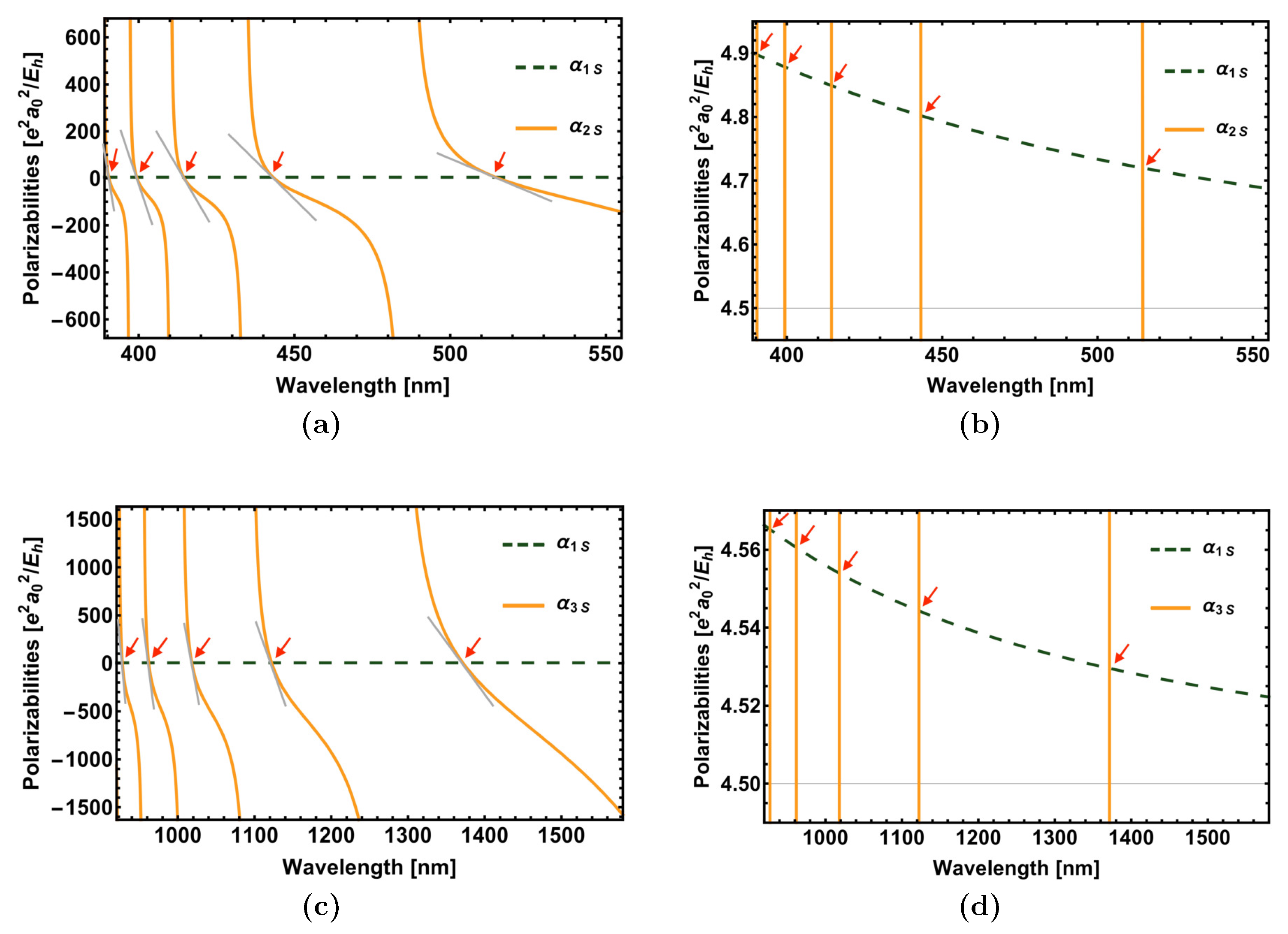
2. Dynamic Polarizability of nS States

We consider the following matrix element of the Schrödinger–Coulomb propagator [23,33,34] of the hydrogen atom, for a reference state $\left|{\varphi }_n\right.〉$,

$$P({\varphi }_n;{\omega }_L)=\frac{e^2}{3}〈{\varphi }_n\left|\overrightarrow{r}\left(\frac{1}{H_s-E_n+\hslash {\omega }_L}\right)\overrightarrow{r}\right|{\varphi }_n〉,$$

(2)

where $\overrightarrow{r}$ is the electron position operator, and $H_s={\overrightarrow{p}}^2/\left(2\mu \right)-e^2/\left(4\pi {ϵ}_{0}r\right)$ is the atomic Schrödinger Hamiltonian. The bound-state energy is $E_n=-\left({\alpha }^2\mu c^2\right)/\left(2n^2\right)$. The momentum operator is denoted as $\overrightarrow{p}$, and the reduced mass of the system is $\mu$. Furthermore, $E_n$ is the energy, and, in the context of the current investigation, ${\omega }_L$ is the angular frequency of the (trapping-field) laser. We use the well-known expression for the Schrödinger–Coulomb bound state ${\Psi }_{n\ell m}\left(\overrightarrow{r}\right)={\Psi }_{n\ell m}(r,\theta ,\phi )=R_{n\ell }\left(r\right)Y_{\ell m}(\theta ,\phi )$ in the coordinate representation,

$$R_{n\ell }\left(r\right)={\left[\frac{(n-\ell -1)!}{(n+\ell )!}\right]}^{1/2}\frac{2^{\ell +1}}{n^2}\frac{1}{{\mathrm{a}}_0^{3/2}}{\left(\frac{r}{n{\mathrm{a}}_0}\right)}^{\ell }exp\left(-\frac{r}{n{\mathrm{a}}_0}\right)L_{n-\ell -1}^{2\ell +1}\left(\frac{2r}{n{\mathrm{a}}_0}\right).$$

(3)

Here,

$${\mathrm{a}}_0=\frac{\hslash }{\alpha \mu c}$$

(4)

is a generalized Bohr radius, adapted to the reduced mass of the system. The spherical harmonic of the angular part is $Y_{\ell m}(\theta ,\phi )$,

$$Y_{\ell m}(\theta ,\phi )={\left[\frac{(2\ell +1)(\ell -m)!}{4\pi (\ell +m)!}\right]}^{1/2}{P}_{\ell }^m\left(cos\left(\theta \right)\right){\mathrm{e}}^{\mathrm{i}m\phi }.$$

(5)

Here, $L_n^{\ell }\left(x\right)$ is the associated Laguerre polynomial, and $P_{\ell }^m\left(cos\left(\theta \right)\right)$ is the associated Legendre polynomial. Also, $n,\ell$ and m are the principal, orbital angular and magnetic orbital quantum numbers, respectively. The Green function $G({\overrightarrow{r}}_1,{\overrightarrow{r}}_2,{\omega }_L)$ of the Schrödinger–Coulomb Hamiltonian $H_s$ fulfills the second-order differential equation:

$$\begin{array}{c}\hfill \left(H_s-E_n+\hslash {\omega }_L\right)G({\overrightarrow{r}}_1,{\overrightarrow{r}}_2,{\omega }_L)={\delta }^{\left(3\right)}({\overrightarrow{r}}_1-{\overrightarrow{r}}_2)\end{array}$$

(6)

and can be expressed in terms of radial Green function $g_{\ell }(r_1,r_2,{\nu }_n)$, and spherical harmonics $Y_{\ell m}({\theta }_i,{\phi }_i)$ as [19]:

$$\begin{array}{c}\hfill G({\overrightarrow{r}}_1,{\overrightarrow{r}}_2,{\nu }_n)=\sum _{\ell =0}^{\infty }\sum _{m=-\ell }^{\ell }{g}_{\ell }(r_1,r_2,{\nu }_n)Y_{\ell m}({\theta }_1,{\phi }_1)Y_{\ell m}^{*}({\theta }_2,{\phi }_2).\end{array}$$

(7)

It is convenient to define the dimensionless energy variable $t_n=t_n\left({\omega }_L\right)$, which parameterizes the laser frequency,

$$t_n\equiv t_n\left({\omega }_L\right)={\left(1+\frac{2n^2\hslash {\omega }_L}{{\alpha }^2\mu c^2}\right)}^{-1/2},{\left[n{t}_n\left({\omega }_L\right)\right]}^2=-\frac{{\alpha }^2\mu c^2}{2(E_n-{\omega }_L)}.$$

(8)

The quantity ${\nu }_n$ acts as a generalization of the principal quantum number n of the reference state, to non-integer ${\nu }_n$, as follows,

$${\nu }_n\equiv {\nu }_n\left({\omega }_L\right)=n{t}_n=n{t}_n\left({\omega }_L\right).$$

(9)

The low-frequency limits are ${\nu }_n\to n$ and $t_n\to 1$ for ${\omega }_L\to 0$, and the high-frequency limit is $t_n\to 0$ for ${\omega }_L\to \infty$. The fine-structure constant is denoted as $\alpha$, and c is the speed of light. In the so-called Sturmian form, the radial Green function $g_{\ell }(r_1,r_2,{\omega }_L)$ can be written as [19,20,21]:

$$\begin{array}{cc}\hfill g_{\ell }(r_1,r_2,{\omega }_L)=& \frac{2\mu }{{\hslash }^2}{\left(\frac{2}{{\mathrm{a}}_0{\nu }_n}\right)}^{2\ell +1}{\left(r_1{r}_2\right)}^{\ell }exp\left(-\frac{r_1+r_2}{{\mathrm{a}}_0{\nu }_n}\right)\hfill \\ \hfill & \times \sum _{k=0}^{\infty }\frac{k!L_k^{2\ell +1}\left(\frac{2r_1}{{\mathrm{a}}_0{\nu }_n}\right)L_k^{2\ell +1}\left(\frac{2r_2}{{\mathrm{a}}_0{\nu }_n}\right)}{(k+2\ell +1)!(k+\ell +1-{\nu }_n)},\hfill \end{array}$$

(10)

where ${\nu }_n\equiv {\nu }_n\left({\omega }_L\right)$. If the reference states is an $nS$ state with $\ell =0$, then one can express Equation (2) in integral form,

$$P({\varphi }_n;{\omega }_L)=\frac{e^2}{3}{\int }_0^{\infty }\mathrm{d}{r}_1{r}_1^3{\int }_0^{\infty }\mathrm{d}{r}_2{r}_2^3{R}_{n0}\left(r_1\right)g_{\ell =1}(r_1,r_2,{\nu }_n=n{t}_n)R_{n0}\left(r_2\right),$$

(11)

where $t_n$ is defined in Equation (8). For a ground state hydrogen ($n=1$), for example, the radial part of the wave function reads $R_{10}\left(r\right)=2{\mathrm{a}}_0^{-3/2}exp(-r/{\mathrm{a}}_0)$. Substituting the radial part $R_{10}\left(r\right)$ and using the Sturmian form of the radial Green function from Equation (10) in Equation (11), one obtains:

$$\begin{array}{cc}\hfill P(1S;{\omega }_L)=& \frac{64\mu e^2}{3{\hslash }^2{\mathrm{a}}_0^6{t}_1^3}{\int }_0^{\infty }{r}_1^4\mathrm{d}{r}_1{\int }_0^{\infty }{r}_2^4\mathrm{d}{r}_{2}exp\left(-\frac{r_1+r_2}{{\mathrm{a}}_0{t}_1}\right)\hfill \\ \hfill & \times exp\left(-\frac{r_1+r_2}{{\mathrm{a}}_0}\right)\sum _{k=0}^{\infty }\frac{k!L_k^3\left(\frac{2r_1}{{\mathrm{a}}_0{t}_1}\right)L_k^3\left(\frac{2r_2}{{\mathrm{a}}_0{t}_1}\right)}{(k+3)!(k+2-t_1)},\hfill \end{array}$$

(12)

which after some algebra works out to [9,24,25,28,29]:

$$\begin{array}{cc}\hfill P(1S;{\omega }_L)=& \frac{{\hslash }^2{e}^2}{{\alpha }^4{\mu }^3{c}^4}[\frac{2t_1^2(-3+3t_1+12t_1^2-12t_1^3-19t_1^4+19t_1^5+26t_1^6+38t_1^7)}{3{(-1+t_1)}^5{(1+t_1)}^4}\hfill \\ \hfill & -\frac{256t_1^9}{3{(-1+t_1)}^5{(1+t_1)}^5}{}_2{F}_1\left(1,-t_1;1-t_1;{\left(\frac{1-t_1}{1+t_1}\right)}^2\right)].\hfill \end{array}$$

(13)

We take the opportunity to correct a sign error in the term multiplying the hypergeometric function in Equation (3a) of Ref. [9]. In the static limit $t_1\to 1$ (${\omega }_L\to 0$), Equation (13) yields half the the static polarizability,

$$P(1S;{\omega }_L\to 0)=\frac{9e^2{\hslash }^2}{4{\alpha }^4{\mu }^3{c}^4}+\mathcal{O}\left({\omega }_L^2\right).$$

(14)

For $t_1\to 0$ (${\omega }_L\to \infty$), the leading asymptotic terms are:

$$\begin{array}{c}\hfill P(1S;{\omega }_L\to \infty )=\frac{3{\hslash }^2{e}^2}{{\alpha }^2{\mu }^2{c}^2}\frac{1}{\hslash {\omega }_L}-\frac{3{\hslash }^2{e}^2}{2\mu }\frac{1}{{\hslash }^2{\omega }_L^2}+\mathcal{O}\left({\omega }_L^{-3}\right).\end{array}$$

(15)

Following the same procedure for $2S$ and $3S$ states, one obtains [9,25,28,29]:

$$\begin{array}{c}P(2S;{\omega }_L)=\frac{{\hslash }^2{e}^2}{{\alpha }^4{\mu }^3{c}^4}[\frac{16t_2^2}{3{(t_2-1)}^6{(t_2+1)}^4}\left(1181t_2^8-314t_2^7-16t_2^6-166t_2^5+14t_2^4+138t_2^3\right.\hfill \\ \hfill \left.-48t_2^2-42t_2+21\right)-\frac{16384t_2^9\left(4t_2^2-1\right)}{3{\left(t_2^2-1\right)}^6}{}_2{F}_1\left(1,-2t_2;1-2t_2;\frac{{(1-t_2)}^2}{{(1+t_2)}^2}\right)],\end{array}$$

(16)

for the $2S$ state. For the $3S$ state, one has the result:

$$\begin{array}{cc}\hfill P_{3S}\left({\omega }_L\right)=& \frac{{\hslash }^2{e}^2}{{\alpha }^4{\mu }^3{c}^4}[\frac{54t_3^2}{{(t_3-1)}^8{(t_3+1)}^6}\left(15538t_3^{12}-2852t_3^{11}-13283t_3^{10}+2090t_3^9\right.\hfill \\ \hfill & \left.+2871t_3^8+40t_3^7-62t_3^6-492t_3^5+128t_3^4+236t_3^3-95t_3^2-46t_3+23\right)\hfill \\ \hfill & -\frac{6912t_3^9{\left(7t_3^2-3\right)}^2\left(9t_3^2-1\right)}{{\left(t_3^2-1\right)}^8}{}_2{F}_1\left(1,-3t_3;1-3t_3;\frac{{(1-t_3)}^2}{{(1+t_3)}^2}\right)].\hfill \end{array}$$

(17)

The dynamical polarizability ${\alpha }_{{\varphi }_n}\left({\omega }_L\right)$ for a reference state ${\varphi }_n$ is the sum:

$$\alpha ({\varphi }_n;{\omega }_L)=P({\varphi }_n;{\omega }_L)+P({\varphi }_n;-{\omega }_L).$$

(18)

As a check, in the static limit, we have $\alpha ({\varphi }_n;{\omega }_L\to 0)=2P({\varphi }_n;{\omega }_L\to 0)$, so that the well-known static polarizability of the ground state:

$$\alpha (1S;{\omega }_L\to 0)=\frac{9e^2{\hslash }^2}{2{\alpha }^4{\mu }^3{c}^4}$$

(19)

is confirmed. The above formalism is adapted to take into account the reduced mass of the system, which is different for hydrogen as opposed to deuterium. If one were to carry out the calculation with the reduced mass $\mu$ of the system being replaced by the electron mass $m_e$, then the appropriate scaling factor for the magic angular frequency is $\mu /m_e$, where $m_e$ is the electron mass. The polarizability itself contains two matrix elements of the position operator, which each scale with the factor $m_e/\mu$, while the propagator denominator scales with $\mu /m_e$, resulting in a total scaling factor ${(m_e/\mu )}^3$ for the polarizability.

3. Magic Wavelength

Whenever the wavelength of an incident laser matches its magic value, the ac Stark shifts of the ground and excited states of a transition become identical. For example, in the transition ${\varphi }_i\to {\varphi }_f$ (initial to final states), we have according to Equation (1),

$$\Delta E_{\mathrm{ac}}({\varphi }_i;{\omega }_L={\omega }_M)=\Delta E_{\mathrm{ac}}({\varphi }_f;{\omega }_L={\omega }_M),$$

(20)

where the magic angular frequency ${\omega }_M$ and the the magic frequency ${\nu }_M$ are given by:

$${\omega }_M=2\pi c/{\lambda }_M,{\nu }_M=c/{\lambda }_M,$$

(21)

respectively. In addition, ${\lambda }_M$ is the magic laser wavelength. In the following, we will use the terms of magic wavelength and magic frequency interchangeably, with the conversion being understood according to Equation (21). For a chosen laser intensity, the ac Stark shift of two levels depends on the polarizabilities of two atomic states. Thus, the magic wavelength ${\lambda }_M$ of the $1S$–$nS$ transition can be determined by the condition:

$${\alpha }_{\Delta }\left({\lambda }_M\right)\equiv \alpha ({\varphi }_f;{\omega }_M)-\alpha ({\varphi }_i;{\omega }_M)=0,$$

(22)

where $|{\varphi }_f\rangle =|nS\rangle$, and $|{\varphi }_i\rangle =|1S\rangle$ or $|2S\rangle$. The quantity ${\nu }_M=c/{\lambda }_M={\omega }_M/\left(2\pi \right)$ gives the magic frequency in Hz (see also

Table 1. The most stable magic wavelengths and slopes at that magic wavelengths for $1S$–$nS$ and $2S$–$nS$ transitions for hydrogen.

Transition	${\mathit{\nu }}_{\mathit{M}}$	${\mathit{\lambda }}_{\mathit{M}}$	$\mathit{\zeta }$	$\mathit{\xi }$	$\mathit{\chi }$
	[${10}^{14}\mathbf{Hz}$ ]	[nm]	[$\mathbf{Hz}\left(\frac{{\mathbf{cm}}^2}{\mathbf{kW}}\right)$]	[$\frac{\mathbf{Hz}}{\mathbf{GHz}}\left(\frac{{\mathbf{cm}}^2}{\mathbf{kW}}\right)$]	[ $\frac{{\mathit{e}}^2{\mathbf{a}}_0^2/{\mathit{E}}_{\mathit{h}}}{\mathbf{nm}}$ ]
$1S$–$2S$	$5.82521$	$514.646$	$-221.58$	$-1.3563$	$-5.2186$
$1S$–$3S$	$2.18531$	$1371.85$	$-212.65$	$-20.192$	$-10.934$
$1S$–$4S$	$1.06583$	$2812.77$	$-211.59$	$-179.26$	$-23.089$
$1S$–$5S$	$0.60703$	$4938.67$	$-211.37$	$-1271.8$	$-53.138$
$1S$–$6S$ (I)	$0.47495$	$6312.10$	$-211.33$	$-1058.6$	$-27.077$
$1S$–$6S$ (II)	$0.42254$	$7094.95$	$-211.32$	$+2445.1$	$+49.501$
$1S$–$7S$	$0.32391$	$9255.47$	$-211.30$	$-5859.6$	$-69.707$
$1S$–$8S$	$0.22944$	$\mathrm{13,066.4}$	$-211.28$	$-\mathrm{18,966}.$	$-113.21$
$2S$–$3S$	$2.20479$	$1359.73$	$-7063.5$	$-24.202$	$-13.340$
$2S$–$4S$	$1.06779$	$2807.60$	$-5909.3$	$-185.94$	$-24.039$
$2S$–$5S$	$0.60730$	$4936.47$	$-5719.7$	$-1287.3$	$-53.831$
$2S$–$6S$ (I)	$0.47527$	$6307.82$	$-5686.1$	$-1077.7$	$-27.603$
$2S$–$6S$ (II)	$0.42241$	$7097.28$	$-5675.0$	$+2494.1$	$+50.459$
$2S$–$7S$	$0.32397$	$9253.80$	$-5657.9$	$-5887.3$	$-70.062$
$2S$–$8S$	$0.22946$	$\mathrm{13,065.4}$	$-5645.9$	$-\mathrm{19,007}$	$-113.47$

and

Table 2. The most stable magic wavelengths and slopes at that magic wavelengths for $1S$–$nS$ and $2S$–$nS$ transitions for deuterium.

Transition	${\mathit{\nu }}_{\mathit{M}}$	${\mathit{\lambda }}_{\mathit{M}}$	$\mathit{\zeta }$	$\mathit{\xi }$	$\mathit{\chi }$
	[${10}^{14}\mathbf{Hz}$ ]	[nm]	[$\mathbf{Hz}\left(\frac{{\mathbf{cm}}^2}{\mathbf{kW}}\right)$]	[$\frac{\mathbf{Hz}}{\mathbf{GHz}}\left(\frac{{\mathbf{cm}}^2}{\mathbf{kW}}\right)$]	[ $\frac{{\mathit{e}}^2{\mathbf{a}}_0^2/{\mathit{E}}_{\mathit{h}}}{\mathbf{nm}}$ ]
$1S$–$2S$	$5.82680$	$514.506$	$-221.40$	$-1.3549$	$-5.2129$
$1S$–$3S$	$2.18590$	$1371.48$	$-212.48$	$-20.171$	$-10.922$
$1S$–$4S$	$1.06612$	$2812.00$	$-211.42$	$-179.06$	$-23.065$
$1S$–$5S$	$0.60720$	$4937.32$	$-211.20$	$-1270.4$	$-53.080$
$1S$–$6S$ (I)	$0.47508$	$6310.38$	$-211.16$	$-1057.5$	$-27.048$
$1S$–$6S$ (II)	$0.42266$	$7093.02$	$-211.15$	$+2442.5$	$+49.447$
$1S$–$7S$	$0.32400$	$9252.95$	$-211.12$	$-5853.2$	$-69.631$
$1S$–$8S$	$0.22950$	$\mathrm{13,062.9}$	$-211.11$	$-\mathrm{18,946}.$	$-113.08$
$2S$–$3S$	$2.20539$	$1359.36$	$-7057.7$	$-24.175$	$-13.325$
$2S$–$4S$	$1.06808$	$2806.84$	$-5904.5$	$-185.74$	$-24.013$
$2S$–$5S$	$0.60747$	$4935.12$	$-5715.1$	$-1285.9$	$-53.773$
$2S$–$6S$ (I)	$0.47540$	$6306.11$	$-5681.4$	$-1076.5$	$-27.573$
$2S$–$6S$ (II)	$0.42252$	$7095.35$	$-5670.4$	$+2491.4$	$+50.404$
$2S$–$7S$	$0.32406$	$9251.28$	$-5653.3$	$-5880.9$	$-69.985$
$2S$–$8S$	$0.22952$	$\mathrm{13,061.8}$	$-5641.2$	$-\mathrm{18,986}.$	$-113.34$

).

The polarizabilities of the ground state and the $2S$ and $3S$ excited states of hydrogen, as a function of the laser wavelength, are shown in Figure 1. The polarizabilities are expressed in atomic units, i.e., in units of $e^2{\mathrm{a}}_0^2/E_h$. Wavelengths are presented in nanometers. Images (a) and (b) of Figure 1 present a general picture of the dynamic polarizabilities with the magic frequencies indicated. Images (b) and (d) of Figure 1 show the polarizabilities near their intersections, i.e., near the magic wavelength. Note that the polarizabilities of the excited states vary over many orders of magnitude over the range of investigated frequencies and becomes singular at resonances, while the ground-state polarizability remains of the same order-of-magnitude as the static value as discussed in Equations (14), (18) and (19).

For reference, in Table 1 and Table 2, we also give the ac Stark shifts, converted to frequency units, of each individual level at the magic wavelength, normalized to the incident trapping laser intensity,

$$\zeta =\frac{1}{h}\frac{1}{I_L}\Delta E_{\mathrm{ac}}({\varphi }_f,{\omega }_M)=\frac{1}{h}\frac{1}{I_L}\Delta E_{\mathrm{ac}}({\varphi }_i,{\omega }_M).$$

(23)

It is essential to ensure the stability of the resonance frequency against small deviations of the trapping laser field from the magic wavelength. The deviation of the ac Stark shift from the zero value attained at the magic wavelength, due to a slight variation of the trapping laser frequency from the magic value, is given as:

$$\xi =\frac{1}{h}\frac{1}{I_L}2\pi {\left.\frac{\partial }{\partial {\omega }_L}\left(\Delta E_{\mathrm{ac}}({\varphi }_f,{\omega }_L)-\Delta E_{\mathrm{ac}}({\varphi }_i,{\omega }_L)\right)\right|}_{{\omega }_L={\omega }_M}$$

(24)

where we refer to Equation (1). The prefactor $1/I_L$ divides out the intensity of the trapping laser, while the other prefactor $1/h$ converts the result to frequency units. Finally, the prefactor $2\pi$ converts the derivative with respect to the angular frequency to a derivative with respect to the trapping laser frequency. Our quantity $\xi$ defined in Equation (24) differs from the quantity $\eta$ defined in Equation (9) of Ref. [9] by a factor $2\pi$. We also take the opportunity to point out that the factor $1/I_L$ was inadvertently omitted from the expression in the middle of Equation (9) of Ref. [9] but is present in the final numerical value presented in Ref. [9]. The unit of $\xi$ is the ac Stark shift, measured in Hz, divided by the deviation of the laser frequency from the magic value, measured in GHz, and the intensity of the exciting laser, measured in kW/cm${}^2$. The unit of $\xi$ is thus $\mathrm{Hz}/(\mathrm{GHz}\mathrm{kW}/{\mathrm{cm}}^2)$.

An alternative method of measuring the deviation is by calculating the change in the polarizability ${\alpha }_{\Delta }$, defined in Equation (22), against variations around the magic wavelength. For convenience, one can divide by the atomic unit of polarizability, which is $e^2{a}_0^2/E_h$, where $E_h$ is the Hartree energy. Then,

$$\chi =\frac{E_h}{e^2{a}_0^2}\left\{{\left.\frac{\partial {\alpha }_{\Delta }\left({\omega }_L\right)}{\partial {\omega }_L}\right|}_{{\omega }_L={\omega }_M}\right\}\frac{\partial {\omega }_M}{\partial {\lambda }_M}=\frac{E_h}{e^2{a}_0^2}\left\{{\left.\frac{\partial {\alpha }_{\Delta }\left({\omega }_L\right)}{\partial {\omega }_L}\right|}_{{\omega }_L={\omega }_M}\right\}\left(-\frac{2\pi c}{{\lambda }_M^2}\right).$$

(25)

The unit of $\chi$ is thus the inverse nanometer, because a dimensionless quantity is differentiated with respect to a wavelength.

According to the intersection points indicated with arrows in Figure 1a, some magic wavelengths for the $2S$–$1S$ transition are close to 514 nm, 443 nm, 414 nm, 399 nm, and 390 nm. One desires a magic wavelength, in which the polarizability has the minimum slope [9]. The polarizability has the minimum slope for the magic wavelength value near 514 nm. Hence it is the most stable one against small deviations of the laser frequency from the magic value (see also Table 1 and Table 2). The wavelength 514 nm lies in between the $2S$–$3P$ hydrogen transition of 656.275 nm and the $2S$–$4P$ transition of 486.132 nm [13,14,35]. This indicates that there is no loss of atoms due to resonant driving. For the $1S$–$3S$ transition in hydrogen, some magic wavelengths are near 1371 nm, 1122 nm, 1018 nm, 961 nm, and 927 nm (see the intersection points indicated with arrows in Figure 1c). The 12-$3S$ hydrogen polarizability difference has the minimum slope value for the 1371.85 nm wavelength, and hence it is the most stable one. Wavelength 1371.85 nm lies in between the $3S$–$4P$ hydrogen transition of 1875.07 nm and the $3S$–$5P$ hydrogen transition of 1281.80 nm [13,14,35], indicating that there is no loss of atoms due to resonant driving. For the $1S$–$6S$ and $2S$–$6S$ transitions, we indicate two alternative magic wavelengths, with commensurate stability coefficients $\xi$ and $\chi$. The smallest magic frequency, for $1S$–$6S$ and $2S$–$6S$, has a somewhat worse stability against deviations frequency instabilities of the trapping laser.

The most stable magic wavelengths and slopes for a various $1S$–$nS$ and $2S$–$nS$ hydrogen and deuterium transitions are listed in Table 1 and Table 2. The magic wavelengths in deuterium are almost the same but slightly smaller than the reduced-mass-corrected value in the analogous transitions in hydrogen. This is because the reduced mass of deuterium is slightly larger than the reduced mass of hydrogen.

4. Relativistic and Field–Configuration Corrections to Magic Wavelengths

A discussion on the accuracy of the result we have obtained is in order. One of the most important corrections comes from the reduced mass of the system, which is in the order of ${10}^{-3}$; this correction is taken into account by the reduced-mass adapted treatment outlined in Section 2. Another important correction is of a relativistic origin. In order to account the relativistic corrections, one should make the following substitution [23] in the $\overrightarrow{r}$-matrix element of the polarizability as:

$$\begin{array}{c}〈{\varphi }_n\left|\overrightarrow{r}\left(\frac{1}{H_s-E_n+\hslash {\omega }_L}\right)\overrightarrow{r}\right|{\varphi }_n〉\to \hfill \\ \hfill 〈{\varphi }_n+\delta {\varphi }_n\left|\overrightarrow{r}\left(\frac{1}{H_s+\delta H-E_n-\delta E_n+\hslash {\omega }_L}\right)\overrightarrow{r}\right|{\varphi }_n+\delta {\varphi }_n〉,\end{array}$$

(26)

where $\delta H$ is the relativistic Hamiltonian correction to the Schrödinger Hamiltonian $H_s$, and $\delta E_n$ is the corresponding relativistic energy correction. Furthermore, $|\delta {\varphi }_n\rangle$ is the relativistic wave function correction. All of these corrections have been discussed in the context of Lamb shift calculations [23]. The relativistic correction is of relative order ${\alpha }^2\sim {10}^{-4}$ and thus suppressed in comparison to the reduced-mass correction [36,37]. The dynamic polarizability and, hence, the magic wavelength also receive field-configuration dependent corrections [5], which depend on the exact position of the atom in the laser field (e.g., whether it is located at a minimum or maximum of the oscillating laser electric field). The field-configuration dependent corrections are also of the order of ${\alpha }^2\sim {10}^{-4}$ [5]. We refrain from a discussion of these effects because the mentioned corrections are not expected to limit experimental precision, in view of the relatively small slopes of the dynamic polarizabilities near the magic wavelengths, as given by the quantities $\xi$ and $\chi$ given in Table 1 and Table 2. The same applies to the hyperpolarizabilities, which give contributions to the fourth-order ac Stark shift [38].

5. Conclusions

We studied the magic wavelengths for the $1S$–$nS$ and $2S$–$nS$ transitions of hydrogen and deuterium. We determined the magic wavelengths in these transitions by calculating the polarizabilities of the atomic states of interest and then finding wavelengths at which the polarizabilities of the respective states cancel in the difference. The polarizabilities are provided by the $nS$ states $\overrightarrow{r}$-matrix elements of the Schrödinger–Coulomb propagator, as discussed in Section 2. Following the determination of the magic wavelengths and corresponding trapping laser frequencies, we calculated the slopes of the dynamic Stark shifts with respect to the frequency of the trapping laser and summarized our results in Table 1 and Table 2. We find that the stability of the elimination of the ac Stark shift against tiny deviations of the trapping laser frequency from the magic value decreases with the increasing quantum number of the excited final state of the transition.

References

1. Bloch, I. Ultracold quantum gases in optical lattices. Nat. Phys. 2005, 1, 23–30. [Google Scholar] [CrossRef]
2. Grimm, R.; Weidemüller, M.; Ovchinnikov, Y.B. Optical Dipole Traps for Neutral Atoms. Adv. At. Mol. Opt. Phys. 2000, 42, 95–170. [Google Scholar]
3. Nicholson, T.L.; Campbell, S.L.; Hutson, R.B.; Marti, G.E.; Bloom, B.J.; McNally, R.L.; Zhang, W.; Barrett, M.D.; Safronova, M.S.; Strouse, G.F.; et al. Systematic evaluation of an atomic clock at 2 × 10⁻¹⁸ total uncertainty. Nat. Commun. 2015, 6, 6896. [Google Scholar] [CrossRef]
4. Katori, H.; Takamoto, M.; Pal’chikov, V.G.; Ovsiannikov, V.D. Ultrastable Optical Clock with Neutral Atoms in an Engineered Light Shift Trap. Phys. Rev. Lett. 2003, 91, 173005. [Google Scholar] [CrossRef] [Green Version]
5. Haas, M.; Jentschura, U.D.; Keitel, C.H.; Kolachevsky, N.; Herrmann, M.; Fendel, P.; Fischer, M.; Udem, T.; Holzwarth, R.; Hänsch, T.W.; et al. Two-photon excitation dynamics in bound two-body Coulomb systems including AC Stark shift and ionization. Phys. Rev. A 2006, 73, 052501. [Google Scholar] [CrossRef] [Green Version]
6. Parthey, C.G.; Matveev, A.; Alnis, J.; Bernhardt, B.; Beyer, A.; Holzwarth, R.; Maistrou, A.; Pohl, R.; Predehl, K.; Udem, T.; et al. Improved Measurement of the Hydrogen 1S–2S Transition Frequency. Phys. Rev. Lett. 2011, 107, 203001. [Google Scholar] [CrossRef] [Green Version]
7. Haas, M.; Jentschura, U.D.; Keitel, C.H. Comparison of classical and second quantized description of the dynamic Stark shift. Am. J. Phys. 2006, 74, 77–81. [Google Scholar] [CrossRef] [Green Version]
8. Kawasaki, A. Magic wavelength for the hydrogen 1S–2S transition. Phys. Rev. A 2015, 92, 042507. [Google Scholar] [CrossRef] [Green Version]
9. Adhikari, C.M.; Kawasaki, A.; Jentschura, U.D. Magic Wavelength for the hydrogen 1S–2S transition: Contribution of the continuum and the reduced-mass correction. Phys. Rev. A 2016, 94, 032510. [Google Scholar] [CrossRef] [Green Version]
10. Ye, J.; Kimble, H.J.; Katori, H. Quantum State Engineering and Precision Metrology Using State-Insensitive Light Traps. Science 2008, 320, 1734–1738. [Google Scholar] [CrossRef] [Green Version]
11. Goldschmidt, E.A.; Norris, D.C.; Koller, S.B.; Wyllie, R.; Brown, R.C.; Porto, J.V.; Safronova, U.I.; Safronova, M.S. Magic wavelengths for the 5s--18s transition in rubidium. Phys. Rev. A 2015, 91, 032518. [Google Scholar] [CrossRef] [Green Version]
12. Yin, D.; Zhang, Y.H.; Li, C.B.; Zhang, X.Z. Magic wavelengths for the 1S--2S and 1S--3S transitions in hydrogen atoms. Chin. Phys. Lett. 2016, 33, 073101. [Google Scholar] [CrossRef]
13. Jentschura, U.D.; Kotochigova, S.; Le Bigot, E.O.; Mohr, P.J.; Taylor, B.N. Precise Calculation of Transition Frequencies of Hydrogen and Deuterium Based on a Least-Squares Analysis. Phys. Rev. Lett. 2005, 95, 163003. [Google Scholar] [CrossRef] [Green Version]
14. For an Interactive Database of Hydrogen and Deuterium Transition Frequencies. Available online: http://physics.nist.gov/hdel (accessed on 10 October 2021).
15. Pachucki, K.; Weitz, M.; Hänsch, T.W. Theory of the hydrogen-deuterium isotope shift. Phys. Rev. A 1994, 49, 2255–2259. [Google Scholar] [CrossRef]
16. Pachucki, K.; Leibfried, D.; Weitz, M.; Huber, A.; König, W.; Hänsch, T.W. Theory of the energy levels and precise two-photon spectroscopy of atomic hydrogen and deuterium. J. Phys. B 1996, 29, 177–195. [Google Scholar] [CrossRef]
17. Parthey, C.G.; Matveev, A.; Alnis, J.; Pohl, R.; Udem, T.; Jentschura, U.D.; Kolachevsky, N.; Hänsch, T.W. Precision Measurement of the Hydrogen-Deuterium 1S–2S Isotope Shift. Phys. Rev. Lett. 2010, 104, 233001. [Google Scholar] [CrossRef]
18. Gavrila, M.; Costescu, A. Retardation in the Elastic Scattering of Photons by Atomic Hydrogen. Phys. Rev. A 1970, 2, 1752–1758, Erratum: Phys. Rev. A 1971, 4, 1688. [Google Scholar] [CrossRef]
19. Swainson, R.A.; Drake, G.W.F. A unified treatment of the non-relativistic and relativistic hydrogen atom I: The wavefunctions. J. Phys. A 1991, 24, 79–94. [Google Scholar] [CrossRef] [Green Version]
20. Swainson, R.A.; Drake, G.W.F. A unified treatment of the non-relativistic and relativistic hydrogen atom II: The Green functions. J. Phys. A 1991, 24, 95–120. [Google Scholar] [CrossRef]
21. Swainson, R.A.; Drake, G.W.F. A unified treatment of the non-relativistic and relativistic hydrogen atom III: The reduced Green functions. J. Phys. A 1991, 24, 1801–1824. [Google Scholar] [CrossRef] [Green Version]
22. Pachucki, K. Higher-Order Binding Corrections to the Lamb Shift. Ann. Phys. 1993, 226, 1–87. [Google Scholar] [CrossRef]
23. Jentschura, U.; Pachucki, K. Higher-order binding corrections to the Lamb shift of 2P states. Phys. Rev. A 1996, 54, 1853–1861. [Google Scholar] [CrossRef] [Green Version]
24. Jentschura, U.D.; Adhikari, C.M.; Debierre, V. Virtual Resonant Emission and Oscillatory Long–Range Tails in van der Waals Interactions of Excited States: QED Treatment and Applications. Phys. Rev. Lett. 2017, 118, 123001. [Google Scholar] [CrossRef] [PubMed]
25. Adhikari, C.M.; Debierre, V.; Matveev, A.; Kolachevsky, N.; Jentschura, U.D. Long-range interactions of hydrogen atoms in excited states. I. 2S–1S interactions and Dirac–δ perturbations. Phys. Rev. A 2017, 95, 022703. [Google Scholar] [CrossRef] [Green Version]
26. Adhikari, C.M.; Debierre, V.; Jentschura, U.D. Adjacency graphs and long-range interactions of atoms in quasi-degenerate states: Applied graph theory. Appl. Phys. B 2017, 123, 1. [Google Scholar] [CrossRef] [Green Version]
27. Jentschura, U.D.; Debierre, V. Long-range tails in van der Waals interactions of excited-state and ground-state atoms. Phys. Rev. A 2017, 95, 042506. [Google Scholar] [CrossRef] [Green Version]
28. Adhikari, C.M. Long-Range Interatomic Interactions: Oscillatory Tails and Hyperfine Perturbations. Ph.D. Thesis, Missouri University of Science and Technology, Rolla, MO, USA, 2017, unpublished. [Google Scholar]
29. Adhikari, C.M.; Debierre, V.; Jentschura, U.D. Long-range interactions of hydrogen atoms in excited states. III. nS–1S interactions for n ≥ 3. Phys. Rev. A 2017, 96, 032702. [Google Scholar] [CrossRef] [Green Version]
30. Jentschura, U.D.; Debierre, V.; Adhikari, C.M.; Matveev, A.; Kolachevsky, N. Long-range interactions of excited hydrogen atoms. II. Hyperfine-resolved 2S–2S system. Phys. Rev. A 2017, 95, 022704. [Google Scholar] [CrossRef] [Green Version]
31. Edmonds, A.R. Angular Momentum in Quantum Mechanics; Princeton University Press: Princeton, NJ, USA, 1957. [Google Scholar]
32. Castillejo, L.; Percival, I.C.; Seaton, M.J. On the Theory of Elastic Collisions Between Electrons and Hydrogen Atoms. Proc. R. Soc. Lond. Ser. A 1960, 254, 259–272. [Google Scholar]
33. Johnson, W.R.; Blundell, S.A.; Sapirstein, J. Finite basis sets for the Dirac equation constructed from B splines. Phys. Rev. A 1988, 37, 307–315. [Google Scholar] [CrossRef]
34. Salomonson, S.; Öster, P. Solution of the pair equation using a finite discrete spectrum. Phys. Rev. A 1989, 40, 5559–5567. [Google Scholar] [CrossRef] [PubMed]
35. Kramida, A.E. A critical compilation of experimental data on spectral lines and energy levels of hydrogen, deuterium, and tritium. At. Data Nucl. Data Tables 2010, 96, 586–644. [Google Scholar] [CrossRef]
36. Anh Thu, L.; Van Hoang, L.; Komarov, L.I.; Romanova, T.S. Relativistic dynamical polarizability of hydrogen-like atoms. J. Phys. B 1996, 91, 2897–2906. [Google Scholar]
37. Yakhontov, V. Relativistic Linear Response Wave Functions and Dynamic Scattering Tensor for the ns1/2-States in Hydrogenlike Atoms. Phys. Rev. Lett. 2003, 91, 093001. [Google Scholar] [CrossRef] [PubMed]
38. Puchalski, M.; Jentschura, U.D.; Mohr, P.J. Blackbody-radiation correction to the polarizability of helium. Phys. Rev. A 2011, 83, 042508. [Google Scholar] [CrossRef] [Green Version]
Figure 1. We investigate the polarizabilities of 1 S and 2 S states of hydrogen as a function of incident wavelength of the incident laser (a) and the same for 1 S and 3 S states of hydrogen (c). Polarizabilities near the points of intersections are shown in (b,d), with the scale of the ordinate axis decreased. Polarizabilities are expressed in atomic units, i.e., in units of e 2 a 0 2 / E h , where a 0 = / ( α m e c ) is the Bohr radius (not adapted to the reduced mass of the system). We recall that the Bohr radius, adapted to the reduced mass, is a 0 = / ( α μ c ) (see Equation (4)). Also, m e is the electron mass, and c is the speed of light. The Hartree energy is E h = α 2 m e c 2 . The wavelengths corresponding to the points of intersection are the magic wavelengths.
Atoms 10 00001 g001